LIGO and Virgo make their data open for anyone to try analysing [bonus note]. If you’re a student looking for a project, a teacher planning a class activity, or a scientist working on a paper, this data is waiting for you to use. Understanding how to analyse the data can be tricky. In this post, I’ll share some of the resources made by LIGO and Virgo to help introduce gravitational-wave analysis. These papers together should give you a good grounding in how to get started working with gravitational-wave data.
If you’d like a more in-depth understanding, I’d recommend visiting your local library for Michele Maggiore’s Gravitational Waves: Volume 1.
It took many decades to develop the technology necessary to build gravitational-wave detectors. Similarly, gravitational-wave data analysis has developed over many decades—I’d say LIGO analysis was really kicked off in the early 1990s by Kipp Thorne’s group. There are now hundreds of papers on various aspects of gravitational-wave analysis. If you are new to the area, where should you start? Don’t panic! For the binary sources discovered so far, this Data Analysis Guide has you covered.
Data from the LIGO and Virgo detectors is released by the Gravitational Wave Open Science Center (GWOSC, pronounced, unfortunately, as it is spelt). If you want to try analysing our delicious data yourself, either searching for signals or studying the signals we have found, GWOSC is the place to start. This paper outlines how these data are produced, going from our laser interferometers to your hard-drive. The paper specifically looks at the data released for our first and second observing runs (O1 and O2), however, GWOSC also host data from the initial detectors’ fifth science run (S5) and sixth science run (S6), and will be updated with new data in the future.
If you do use data from GWOSC, please remember to say thank you.
Synopsis:Data Analysis Guide Read this if: You want an introduction to signal analysis Favourite part: This is a great resource for new students [bonus note]
Gravitational-wave detectors measure ripples in spacetime. They record a simple time series of the stretching and squeezing of space as a gravitational wave passes. Well, they measure that, plus a whole lot of noise. Most of the time it is just noise. How do we go from this time series to discoveries about the Universe’s black holes and neutron stars? This paper gives the outline, it covers (in order)
An introduction to observations at the time of writing
The basics of LIGO and Virgo data—what it is the we analyse
The basics of detector noise—how we describe sources of noise in our data
Fourier analysis—how we go from time series to looking at the data in the as a function of frequency, which is the most natural way to analyse that data.
Time–frequency analysis and stationarity—how we check the stability of data from our detectors
Detector calibration and data quality—how we make sure we have good quality data
The noise model and likelihood—how we use our understanding of the noise, under the assumption of it being stationary, to work out the likelihood of different signals being in the data
Signal detection—how we identify times in the data which have a transient signal present
Inferring waveform and physical parameters—how we estimate the parameters of the source of a gravitational wave
Residuals around GW150914—a consistency check that we have understood the noise surrounding our first detection
The paper works through things thoroughly, and I would encourage you to work though it if you are interested.
I won’t summarise everything here, I want to focus the (roughly undergraduate-level) foundations of how we do our analysis in the frequency domain. My discussion of the GWOSC Paper goes into more detail on the basics of LIGO and Virgo data, and some details on calibration and data quality. I’ll leave talking about residuals to this bonus note, as it involves a long tangent and me needing to lie down for a while.
Fourier analysis
The signal our detectors measure is a time series . This is may just contain noise, , or it may also contain a signal, .
There are many sources of noise for our detectors. The different sources can affect different frequencies. If we assume that the noise is stationary, so that it’s properties don’t change with time, we can simply describe the properties of the noise with the power spectral density. On average we expect the noise at a given frequency to be zero, but with it fluctuating up and down with a variance given by the power spectral density. We typically approximate the noise as Gaussian, such that
,
where we use to represent a normal distribution with mean and standard deviation . The approximations of stationary and Gaussian noise are good most of the time. The noise does vary over time, but is usually effectively stationary over the durations we look at for a signal. The noise is also mostly Gaussian except for glitches. These are taken into account when we search for signals, but we’ll ignore them for now. The statistical description of the noise in terms of the power spectral density allows us to understand our data, but this understanding comes as a function of frequency: we must transform of time domain data to frequency domain data.
The go from to we can use a Fourier transform. Fourier transforms are a way of converting a function of one variable into a function of a reciprocal variable—in the case of time you convert to frequency. Fourier transforms encode all the information of the original function, so it is possible to convert back and forth as you like. Really, a Fourier transform is just another way of looking at the same function.
The Fourier transform is defined as
.
Now, from this you might notice a problem when it comes to real data analysis, namely that the integral is defined over an infinite amount of time. We don’t have that much data. Instead, we only have a short period.
We could recast the integral above over a shorter time if instead of taking the Fourier transform of , we take the Fourier transform of where is some window function which goes to zero outside of the time interval we are looking at. What we end up with is a convolution of the function we want with the Fourier transform of the window function,
.
It is important to pick a window function which minimises the distortion to the signal that we want. If we just take a tophat (also known as a boxcar or rectangular, possibly on account of its infamous criminal background) function which is abruptly cuts off the data at the ends of the time interval, we find that is a sinc function. This is not a good thing, as it leads to all sorts of unwanted correlations between different frequencies, commonly known as spectral leakage. A much better choice is a function which smoothly tapers to zero at the edges. Using a tapering window, we lose a little data at the edges (we need to be careful choosing the length of the data analysed), but we can avoid the significant nastiness of spectral leakage. A tapering window function should always be used. Then or finite-time Fourier transform is then a good approximation to the exact .
Data processing to reveal GW150914. The top panel shows raw Hanford data. The second panel shows a window function being applied. The third panel shows the data after being whitened. This cleans up the data, making it easier to pick out the signal from all the low frequency noise. The bottom panel shows the whitened data after a bandpass filter is applied to pick out the signal. We don’t use the bandpass filter in our analysis (it is just for illustration), but the other steps reflect how we treat our data. Figure 2 of the Data Analysis Guide.
Now we have our data in the frequency domain, it is simple enough to compare the data to the expected noise a t a given frequency. If we measure something loud at a frequency with lots of noise we should be less surprised than if we measure something loud at a frequency which is usually quiet. This is kind of like how somewhat shouting is less startling at a rock concert than in a library. The appropriate way to weight is to divide by the square root of power spectral density . This is known as whitening. Whitened data should have equal amplitude fluctuations at all frequencies, allowing for easy comparisons.
Now we understand the statistical properties of noise we can do some analysis! We can start by testing our assumption that the data are stationary and Gaussian by checking that that after whitening we get the expected distribution. We can also define the likelihood of obtaining the data given a model of a gravitational-wave signal , as the properties of the noise mean that . Combining the likelihood for each individual frequency gives the overall likelihood
.
This likelihood is at the heart of parameter estimation, as we can work out the probability of there being a signal with a given set of parameters. The Data Analysis Guide goes through many different analyses (including parameter estimation) and demonstrates how to check that noise is nice and Gaussian.
Distribution of residuals for 4 seconds of data around GW150914 after subtracting the maximum likelihood waveform. The residuals are the whitened Fourier amplitudes, and they should be consistent with a unit Gaussian. The residuals follow the expected distribution and show no sign of non-Gaussianity. Figure 14 of the Data Analysis Guide.
Synopsis:GWOSC Paper Read this if: You want to analyse our gravitational wave data Favourite part: All the cool projects done with this data
You’re now up-to-speed with some ideas of how to analyse gravitational-wave data, you’ve made yourself a fresh cup of really hot tea, you’re ready to get to work! All you need are the data—this paper explains where this comes from.
Data production
The first step in getting gravitational-wave data is the easy one. You need to design a detector, convince science agencies to invest something like half a billion dollars in building one, then spend 40 years carefully researching the necessary technology and putting it all together as part of an international collaboration of hundreds of scientists, engineers and technicians, before painstakingly commissioning the instrument and operating it. For your convenience, we have done this step for you, but do feel free to try it yourself at home.
Gravitational-wave detectors like Advanced LIGO are built around an interferometer: they have two arms at right angles to each other, and we bounce lasers up and down them to measure their length. A passing gravitational wave will change the relative length of one arm relative to the other. This changes the time taken to travel along one arm compared to the other. Hence, when the two bits of light reach the output of the interferometer, they’ll have a different phase:where normally one light wave would have a peak, it’ll have a trough. This change in phase will change how light from the two arms combine together. When no gravitational wave is present, the light interferes destructively, almost cancelling out so that the output is dark. We measure the brightness of light at the output which tells us about how the length of the arms changes.
We want our detector in measure the gravitational-wave strain. That is the fractional change in length of the arms,
,
where is the relative difference in the length of the two arms, and is the usually arm length. Since we love jargon in LIGO & Virgo, we’ll often refer to the strain as HOFT (as you would read as h of t; it took me years to realise this) or DARM (differential arm measurement).
The actual output of the detector is the voltage from a photodiode measuring the intensity of the light. It is necessary to make careful calibration of the detectors. In theory this is simple: we change the position of the mirrors at the end of the arms and see how the output changes. In practise, it is very difficult. The GW150914 Calibration Paper goes into details for O1, more up-to-date descriptions are given in Cahillane et al. (2017) for LIGO and Acernese et al. (2018) for Virgo. The calibration of the detectors can drift over time, improving the calibration is one of the things we do between originally taking the data and releasing the final data.
The data are only celebrated between 10 Hz and 5 kHz, so don’t trust the data outside of that frequency range.
The next stage of our data’s journey is going through detector characterisation and data quality checks. In addition to measuring gravitational-wave strain, we record many other data channels: about 200,000 per detector. These measure all sorts of things, from the internal state of the instrument, to monitoring the physical environment around the detectors. These auxiliary channels are used to check the data quality. In some cases, an auxiliary channel will record a source of noise, like scattered light or the mains power frequency, allowing us to clean up our strain data by subtracting out this noise. In other cases, an auxiliary channel can act as a witness to a glitch in our detector, identifying when it is misbehaving so that we know not to trust that part of the data. The GW150914 Detector Characterisation Paper goes into details of how we check potential detections. In doing data quality checks we are careful to only use the auxiliary channels which record something which would be independent of a passing gravitational wave.
We have 4 flags for data quality:
DATA: All clear. Certified fresh. Eat as much as you like.
CAT1: A critical problem with the instrument. Data from these times are likely to be a dumpster fire of noise. We do not use them in our analyses, and they are currently excluded from our public releases. About 1.7% of Hanford data and 1.0% of time from Livingston was flagged with CAT1 in O1. In O2, we got this done to 0.001% for Hanford, 0.003% for Livingston and 0.05% for Virgo.
CAT2: Some activity in an auxiliary channel (possibly the electric boogaloo monitor) which has a well understood correlation with the measured strain channel. You would therefore expect to find some form of glitchiness in the data.
CAT3: There is some correlation in an auxiliary channel and the strain channel which is not understood. We’re not currently using this flag, but it’s kept as an option.
It’s important to verify the data quality before starting your analysis. You don’t want to get excited to discover a completely new form of gravitational wave only to realise that it’s actually some noise from nearby logging. Remember, if a tree falls in the forest and no-one is around, LIGO will still know.
To test our systems, we also occasionally perform a signal injection: we move the mirrors to simulate a signal. This is useful for calibration and for testing analysis algorithms. We don’t perform injections very often (they get in the way of looking for real signals), but these times are flagged. Just as for data quality flags, it is important to check for injections before analysing a stretch of data.
Once passing through all these checks, the data is ready to analyse!
After our data have been lovingly prepared, they are served up in two data formats:
Hierarchical Data Format HDF, which is a popular data storage format, as it is easily allows for metadata and multiple data sets (like the important data quality flags) to be packaged together.
Gravitational Wave Frame GWF, which is the standard format we use internally. Veteran gravitational-wave scientists often get a far-way haunted look when you bring up how the specifications for this file format were decided. It’s best not to mention unless you are also buying them a stiff drink.
In these files, you will find sampled at either 4096 Hz or 16384 Hz (either are available). Pick the sampling rate you need depending upon the frequency range you are interested in: the 4096 Hz data are good for upto 1.7 kHz, while the 16384 Hz are good to the limit of the calibration range at 5 kHz.
Files can be downloaded from the GWOSC website. If you want to download a large amount, it is recommended to use the CernVM-FS distributed file system.
To check when the gravitational-wave detectors were observing, you can use the Timeline search.
Screenshot of the GWOSC Timeline showing observing from the fifth science run (S5) on the initial detector era through to the second observing run (O2) of the advanced detector era. Bars show observing of GEO 600 (G1), Hanford (H1 and H2), Livingston (L1) and Virgo (V1). Hanford initial had two detectors housed within its site, the plan in the advanced detector era is to install the equipment as LIGO India instead.
Try this at home
Having gone through all these details, you should now know what are data is, over what ranges it can be analyzed, and how to get access to it. Your cup of tea has also probably gone cold. Why not make yourself a new one, and have a couple of biscuits as reward too. You deserve it!
In a chunk surrounding an event at time of publication of that event. This enables the new detection to be analysed by anyone. We typically release about an hour of data around an event.
18 months after the end of the run. This time gives us chance to properly calibrate the data, check the data quality, and then run the analyses we are committed to. A lot of work goes into producing gravitational wave data!
Start marking your calendars now for the release of O3 data.
Summer studenting
In summer 2019, while we were finishing up on the Data Analysis Guide, I gave it to one of my summer students Andrew Kim as an introduction. Andrew was working on gravitational-wave data analysis, so I hoped that he’d find it useful. He ended up working through the draft notebook made to accompany the paper and making a number of useful suggestions! He ended up as an author on the paper because of these contributions, which was nice.
The conspiracy of residuals
The Data Analysis Guide is an extremely useful paper. It explains many details of gravitational-wave analysis. The detections made by LIGO and Virgo over the last few years has increased the interest in analysing gravitational waves, making it the perfect time to write such an article. However, that’s not really what motivated us to write it.
In 2017, a paper appeared on the arXiv making claims of suspicious correlations in our LIGO data around GW150914. Could this call into question the very nature of our detection? No. The paper has two serious flaws.
The first argument in the paper was that there were suspicious phase correlations in the data. This is because the authors didn’t window their data before Fourier transforming.
The second argument was the residuals presented in Figure 1 of the GW150914 Discovery Paper contain a correlation. This is true, but these residuals aren’t actually the results of how we analyse the data. The point of Figure 1 was to that you don’t need our fancy analysis to see the signal—you can spot it by eye. Unfortunately, doing things by eye isn’t perfect, and this imperfection was picked up on.
The first flaw is a rookie mistake—pretty much everyone does it at some point. I did it starting out as a first-year PhD student, and I’ve run into it with all the undergraduates I’ve worked with writing their own analyses. The authors of this paper are rookies in gravitational-wave analysis, so they shouldn’t be judged too harshly for falling into this trap, and it is something so simple I can’t blame the referee of the paper for not thinking to ask. Any physics undergraduate who has met Fourier transforms (the second year of my degree) should grasp the mistake—it’s not something esoteric you need to be an expert in quantum gravity to understand.
The second flaw is something which could have been easily avoided if we had been more careful in the GW150914 Discovery Paper. We could have easily aligned the waveforms properly, or more clearly explained that the treatment used for Figure 1 is not what we actually do. However, we did write many other papers explaining what we did do, so we were hardly being secretive. While Figure 1 was not perfect, it was not wrong—it might not be what you might hope for, but it is described correctly in the text, and none of the LIGO–Virgo results depend on the figure in any way.
Recovered gravitational waveforms from our analysis of GW150914. The grey line shows the data whitened by the noise spectrum. The dark band shows our estimate for the waveform without assuming a particular source. The light bands show results if we assume it is a binary black hole (BBH) as predicted by general relativity. This plot more accurately represents how we analyse gravitational-wave data. Figure 6 of the GW150914 Parameter Estimation Paper.
Both mistakes are easy to fix. They are at the level of “Oops, that’s embarrassing! Give me 10 minutes. OK, that looks better”. Unfortunately, that didn’t happen.
The paper regrettably got picked up by science blogs, and caused much of a flutter. There were demands that LIGO and Virgo publically explain ourselves. This was difficult—the Collaboration is set up to do careful science, not handle a PR disaster. One of the problems was that we didn’t want to be seen to policing the use of our data. We can’t check that every paper ever using our data does everything perfectly. We don’t have time, and that probably wouldn’t encourage people to use our data if they knew any mistake would be pulled up by this 1000 person collaboration. A second problem was that getting anything approved as an official Collaboration document takes ages—getting consensus amongst so many people isn’t always easy. What would you do—would you want to be the faceless Collaboration persecuting the helpless, plucky scientists trying to check results?
There were private communications between people in the Collaboration and the authors. It took us a while to isolate the sources of the problems. In the meantime, pressure was mounting for an official™ response. It’s hard to justify why your analysis is correct by gesturing to a stack of a dozen papers—people don’t have time to dig through all that (I actually sent links to 16 papers to a science journalist who contacted me back in July 2017). Our silence may have been perceived as arrogance or guilt.
It was decided that we would put out an unofficial response. Ian Harry had been communicating with the authors, and wrote up his notes which Sean Carroll kindly shared on his blog. Unfortunately, this didn’t really make anyone too happy. The authors of the paper weren’t happy that something was shared via such an informal medium; the post is too technical for the general public to appreciate, and there was a minor typo in the accompanying code which (since fixed) was seized upon. It became necessary to write a formal paper.
We did continue to try to explain the errors to the authors. I have colleagues who spent many hours in a room in Copenhagen trying to explain the mistakes. However, little progress was made, and it was not a fun time™. I can imagine at this point that the authors of the paper were sufficiently angry not to want to listen, which is a shame.
Now that the Data Analysis Guide is published, everyone will be satisfied, right? A refereed journal article should quash all fears, surely? Sadly, I doubt this will be the case. I expect these doubts will keep circulating for years. After all, there are those who still think vaccines cause autism. Fortunately, not believing in gravitational waves won’t kill any children. If anyone asks though, you can tell them that any doubts on LIGO’s analysis have been quashed, and that vaccines cause adults!
For a good account of the back and forth, Natalie Wolchover wrote a nice article in Quanta, and for a more acerbic view, try Mark Hannam’s blog.
After three months (and one binary black hole detection announcement), I finally have time to write about the suite of LIGO–Virgo papers put together to accompany GW170817.
The papers
There are currently 9 papers in the GW170817 family. Further papers, for example looking at parameter estimation in detail, are in progress. Papers are listed below in order of arXiv posting. My favourite is the GW170817 Discovery Paper. Many of the highlights, especially from the Discovery and Multimessenger Astronomy Papers, are described in my GW170817 announcement post.
Keeping up with all the accompanying observational results is a task not even Sisyphus would envy. I’m sure that the details of these will be debated for a long time to come. I’ve included references to a few below (mostly as [citation notes]), but these are not guaranteed to be complete (I’ll continue to expand these in the future).
This is the paper announcing the gravitational-wave detection. It gives an overview of the properties of the signal, initial estimates of the parameters of the source (see the GW170817 Properties Paper for updates) and the binary neutron star merger rate, as well as an overview of results from the other companion papers.
I was disappointed that “the era of gravitational-wave multi-messenger astronomy has opened with a bang” didn’t make the conclusion of the final draft.
I’ve numbered this paper as −1 as it gives an overview of all the observations—gravitational wave, electromagnetic and neutrino—accompanying GW170817. I feel a little sorry for the neutrino observers, as they’re the only ones not to make a detection. Drawing together the gravitational wave and electromagnetic observations, we can confirm that binary neutron star mergers are the progenitors of (at least some) short gamma-ray bursts and kilonovae.
Do not print this paper, the author list stretches across 23 pages.
Here we bring together the LIGO–Virgo observations of GW170817 and the Fermi and INTEGRAL observations of GRB 170817A. From the spatial and temporal coincidence of the gravitational waves and gamma rays, we establish that the two are associated with each other. There is a 1.7 s time delay between the merger time estimated from gravitational waves and the arrival of the gamma-rays. From this, we make some inferences about the structure of the jet which is the source of the gamma rays. We can also use this to constrain deviations from general relativity, which is cool. Finally, we estimate that there be 0.3–1.7 joint gamma ray–gravitational wave detections per year once our gravitational-wave detectors reach design sensitivity!
The Hubble constant quantifies the current rate of expansion of the Universe. If you know how far away an object is, and how fast it is moving away (due to the expansion of the Universe, not because it’s on a bus or something, that is important), you can estimate the Hubble constant. Gravitational waves give us an estimate of the distance to the source of GW170817. The observations of the optical transient AT 2017gfo allow us to identify the galaxy NGC 4993 as the host of GW170817’s source. We know the redshift of the galaxy (which indicates how fast its moving). Therefore, putting the two together we can infer the Hubble constant in a completely new way.
During the coalescence of two neutron stars, lots of neutron-rich matter gets ejected. This undergoes rapid radioactive decay, which powers a kilonova, an optical transient. The observed signal depends upon the material ejected. Here, we try to use our gravitational-wave measurements to predict the properties of the ejecta ahead of the flurry of observational papers.
We can detect signals if they are loud enough, but there will be many quieter ones that we cannot pick out from the noise. These add together to form an overlapping background of signals, a background rumbling in our detectors. We use the inferred rate of binary neutron star mergers to estimate their background. This is smaller than the background from binary black hole mergers (black holes are more massive, so they’re intrinsically louder), but they all add up. It’ll still be a few years before we could detect a background signal.
We know that GW170817 came from the coalescence of two neutron stars, but where did these neutron stars come from? Here, we combine the parameters inferred from our gravitational-wave measurements, the observed position of AT 2017gfo in NGC 4993 and models for the host galaxy, to estimate properties like the kick imparted to neutron stars during the supernova explosion and how long it took the binary to merge.
This is the search for neutrinos from the source of GW170817. Lots of neutrinos are emitted during the collision, but not enough to be detectable on Earth. Indeed, we don’t find any neutrinos, but we combine results from three experiments to set upper limits.
After the two neutron stars merged, what was left? A larger neutron star or a black hole? Potentially we could detect gravitational waves from a wibbling neutron star, as it sloshes around following the collision. We don’t. It would have to be a lot closer for this to be plausible. However, this paper outlines how to search for such signals; the GW170817 Properties Paper contains a more detailed look at any potential post-merger signal.
Title: Properties of the binary neutron star merger GW170817
arXiv:1805.11579 [gr-qc]
In the GW170817 Discovery Paper we presented initial estimates for the properties of GW170817’s source. These were the best we could do on the tight deadline for the announcement (it was a pretty good job in my opinion). Now we have had a bit more time we can present a new, improved analysis. This uses recalibrated data and a wider selection of waveform models. We also fold in our knowledge of the source location, thanks to the observation of AT 2017gfo by our astronomer partners, for our best results. if you want to know the details of GW170817’s source, this is the paper for you!
If you’re looking for the most up-to-date results regarding GW170817, check out the O2 Catalogue Paper.
Title: GW170817: Measurements of neutron star radii and equation of state
arXiv:1805.11581 [gr-qc]
Neutron stars are made of weird stuff: nuclear density material which we cannot replicate here on Earth. Neutron star matter is often described in terms of an equation of state, a relationship that explains how the material changes at different pressures or densities. A stiffer equation of state means that the material is harder to squash, and a softer equation of state is easier to squish. This means that for a given mass, a stiffer equation of state will predict a larger, fluffier neutron star, while a softer equation of state will predict a more compact, denser neutron star. In this paper, we assume that GW170817’s source is a binary neutron star system, where both neutron stars have the same equation of state, and see what we can infer about neutron star stuff™.
Synopsis:GW170817 Discovery Paper Read this if: You want all the details of our first gravitational-wave observation of a binary neutron star coalescence Favourite part: Look how well we measure the chirp mass!
GW170817 was a remarkable gravitational-wave discovery. It is the loudest signal observed to date, and the source with the lowest mass components. I’ve written about some of the highlights of the discovery in my previous GW170817 discovery post.
Binary neutron stars are one of the principal targets for LIGO and Virgo. The first observational evidence for the existence of gravitational waves came from observations of binary pulsars—a binary neutron star system where (at least one) one of the components is a pulsar. Therefore (unlike binary black holes), we knew that these sources existed before we turned on our detectors. What was less certain was how often they merge. In our first advanced-detector observing run (O1), we didn’t find any, allowing us to estimate an upper limit on the merger rate of . Now, we know much more about merging binary neutron stars.
GW170817, as a loud and long signal, is a highly significant detection. You can see it in the data by eye. Therefore, it should have been a easy detection. As is often the case with real experiments, it wasn’t quite that simple. Data transfer from Virgo had stopped over night, and there was a glitch (a non-stationary and non-Gaussian noise feature) in the Livingston detector, which meant that this data weren’t automatically analysed. Nevertheless, GstLAL flagged something interesting in the Hanford data, and there was a mad flurry to get the other data in place so that we could analyse the signal in all three detectors. I remember being sceptical in these first few minutes until I saw the plot of Livingston data which blew me away: the chirp was clearly visible despite the glitch!
Time–frequency plots for GW170104 as measured by Hanford, Livingston and Virgo. The Livingston data have had the glitch removed. The signal is clearly visible in the two LIGO detectors as the upward sweeping chirp; it is not visible in Virgo because of its lower sensitivity and the source’s position in the sky. Figure 1 of the GW170817 Discovery Paper.
Using data from both of our LIGO detectors (as discussed for GW170814, our offline algorithms searching for coalescing binaries only use these two detectors during O2), GW170817 is an absolutely gold-plated detection. GstLAL estimates a false alarm rate (the rate at which you’d expect something at least this signal-like to appear in the detectors due to a random noise fluctuation) of less than one in 1,100,000 years, while PyCBC estimates the false alarm rate to be less than one in 80,000 years.
Parameter estimation (inferring the source properties) used data from all three detectors. We present a (remarkably thorough given the available time) initial analysis in this paper (more detailed results are given in the GW170817 Properties Paper, and the most up-to-date results are in O2 Catalogue Paper). This signal is challenging to analyse because of the glitch and because binary neutron stars are made of stuff™, which can leave an imprint on the waveform. We’ll be looking at the effects of these complications in more detail in the future. Our initial results are
The source is localized to a region of about at a distance of (we typically quote results at the 90% credible level). This is the closest gravitational-wave source yet.
The chirp mass is measured to be , much lower than for our binary black hole detections.
The spins are not well constrained, the uncertainty from this means that we don’t get precise measurements of the individual component masses. We quote results with two choices of spin prior: the astrophysically motivated limit of 0.05, and the more agnostic and conservative upper bound of 0.89. I’ll stick to using the low-spin prior results be default.
Using the low-spin prior, the component masses are – and –. We have the convention that , which is why the masses look unequal; there’s a lot of support for them being nearly equal. These masses match what you’d expect for neutron stars.
As mentioned above, neutron stars are made of stuff™, and the properties of this leave an imprint on the waveform. If neutron stars are big and fluffy, they will get tidally distorted. Raising tides sucks energy and angular momentum out of the orbit, making the inspiral quicker. If neutron stars are small and dense, tides are smaller and the inspiral looks like that for tow black holes. For this initial analysis, we used waveforms which includes some tidal effects, so we get some preliminary information on the tides. We cannot exclude zero tidal deformation, meaning we cannot rule out from gravitational waves alone that the source contains at least one black hole (although this would be surprising, given the masses). However, we can place a weak upper limit on the combined dimensionless tidal deformability of . This isn’t too informative, in terms of working out what neutron stars are made from, but we’ll come back to this in the GW170817 Properties Paper and the GW170817 Equation-of-state Paper.
Given the source masses, and all the electromagnetic observations, we’re pretty sure this is a binary neutron star system—there’s nothing to suggest otherwise.
Having observed one (and one one) binary neutron star coalescence in O1 and O2, we can now put better constraints on the merger rate. As a first estimate, we assume that component masses are uniformly distributed between and , and that spins are below 0.4 (in between the limits used for parameter estimation). Given this, we infer that the merger rate is , safely within our previous upper limit [citation note].
There’s a lot more we can learn from GW170817, especially as we don’t just have gravitational waves as a source of information, and this is explained in the companion papers.
The Multimessenger Paper
Synopsis:Multimessenger Paper Read this if: Don’t. Use it too look up which other papers to read. Favourite part: The figures! It was a truly amazing observational effort to follow-up GW170817
The remarkable thing about this paper is that it exists. Bringing together such a diverse (and competitive) group was a huge effort. Alberto Vecchio was one of the editors, and each evening when leaving the office, he was convinced that the paper would have fallen apart by morning. However, it hung together—the story was too compelling. This paper explains how gravitational waves, short gamma-ray bursts, kilonovae all come from a single source [citation note]. This is the greatest collaborative effort in the history of astronomy.
The paper outlines the discoveries and all of the initial set of observations. If you want to understand the observations themselves, this is not the paper to read. However, using it, you can track down the papers that you do want. A huge amount of care went in to trying to describe how discoveries were made: for example, Fermi observed GRB 170817A independently of the gravitational-wave alert, and we found GW170817 without relying on the GRB alert, however, the communication between teams meant that we took everything much seriously and pushed out alerts as quickly as possible. For more on the history of observations, I’d suggest scrolling through the GCN archive.
The paper starts with an overview of the gravitational-wave observations from the inspiral, then the prompt detection of GRB 170817A, before describing how the gravitational-wave localization enabled discovery of the optical transient AT 2017gfo. This source, in nearby galaxy NGC 4993, was then the subject of follow-up across the electromagnetic spectrum. We have huge amount of photometric and spectroscopy of the source, showing general agreement with models for a kilonova. X-ray and radio afterglows were observed 9 days and 16 days after the merger, respectively [citation note]. No neutrinos were found, which isn’t surprising.
The GW170817 Gamma-ray Burst Paper
Synopsis:GW170817 Gamma-ray Burst Paper Read this if: You’re interested in the jets from where short gamma-ray bursts originate or in tests of general relativity Favourite part: How much science come come from a simple time delay measurement
This joint LIGO–Virgo–Fermi–INTEGRAL paper combines our observations of GW170817 and GRB 170817A. The result is one of the most contentful of the companion papers.
Detection of GW170817 and GRB 170817A. The top three panels show the gamma-ray lightcurves (first: GBM detectors 1, 2, and 5 for 10–50 keV; second: GBM data for 50–300 keV ; third: the SPI-ACS data starting approximately at 100 keV and with a high energy limit of least 80 MeV), the red line indicates the background.The bottom shows the a time–frequency representation of coherently combined gravitational-wave data from LIGO-Hanford and LIGO-Livingston. Figure 2 of the GW170817 Gamma-ray Burst Paper.
The first item on the to-do list for joint gravitational-wave–gamma-ray science, is to establish that we are really looking at the same source.
From the GW170817 Discovery Paper, we know that its source is consistent with being a binary neutron star system. Hence, there is matter around which can launch create the gamma-rays. The Fermi-GBM and INTEGRAL observations of GRB170817A indicate that it falls into the short class, as hypothesised as the result of a binary neutron star coalescence. Therefore, it looks like we could have the right ingredients.
Now, given that it is possible that the gravitational waves and gamma rays have the same source, we can calculate the probability of the two occurring by chance. The probability of temporal coincidence is , adding in spatial coincidence too, and the probability becomes . It’s safe to conclude that the two are associated: merging binary neutron stars are the source of at least some short gamma-ray bursts!
Testing gravity
There is a delay time between the inferred merger time and the gamma-ray burst. Given that signal has travelled for about 85 million years (taking the 5% lower limit on the inferred distance), this is a really small difference: gravity and light must travel at almost exactly the same speed. To derive exact limit you need to make some assumptions about when the gamma-rays were created. We’d expect some delay as it takes time for the jet to be created, and then for the gamma-rays to blast their way out of the surrounding material. We conservatively (and arbitrarily) take a window of the delay being 0 to 10 seconds, this gives
.
That’s pretty small!
General relativity predicts that gravity and light should travel at the same speed, so I wasn’t too surprised by this result. I was surprised, however, that this result seems to have caused a flurry of activity in effectively ruling out several modified theories of gravity. I guess there’s not much point in explaining what these are now, but they are mostly theories which add in extra fields, which allow you to tweak how gravity works so you can explain some of the effects attributed to dark energy or dark matter. I’d recommend Figure 2 of Ezquiaga & Zumalacárregui (2017) for a summary of which theories pass the test and which are in trouble; Kase & Tsujikawa (2018) give a good review.
Table showing viable (left) and non-viable (right) scalar–tensor theories after discovery of GW170817/GRB 170817A. The theories are grouped as Horndeski theories and (the more general) beyond Horndeski theories. General relativity is a tensor theory, so these models add in an extra scalar component. Figure 2 of Ezquiaga & Zumalacárregui (2017).
We don’t discuss the theoretical implications of the relative speeds of gravity and light in this paper, but we do use the time delay to place bounds for particular on potential deviations from general relativity.
We look at a particular type of Lorentz invariance violation. This is similar to what we did for GW170104, where we looked at the dispersion of gravitational waves, but here it is for the case of , which we couldn’t test.
We look at the Shapiro delay, which is the time difference travelling in a curved spacetime relative to a flat one. That light and gravity are effected the same way is a test of the weak equivalence principle—that everything falls the same way. The effects of the curvature can be quantified with the parameter , which describes the amount of curvature per unit mass. In general relativity . Considering the gravitational potential of the Milky Way, we find that [citation note].
As you’d expect given the small time delay, these bounds are pretty tight! If you’re working on a modified theory of gravity, you have some extra checks to do now.
Gamma-ray bursts and jets
From our gravitational-wave and gamma-ray observations, we can also make some deductions about the engine which created the burst. The complication here, is that we’re not exactly sure what generates the gamma rays, and so deductions are model dependent. Section 5 of the paper uses the time delay between the merger and the burst, together with how quickly the burst rises and fades, to place constraints on the size of the emitting region in different models. The papers goes through the derivation in a step-by-step way, so I’ll not summarise that here: if you’re interested, check it out.
Isotropic energies (left) and luminosities (right) for all gamma-ray bursts with measured distances. These isotropic quantities assume equal emission in all directions, which gives an upper bound on the true value if we are observing on-axis. The short and long gamma-ray bursts are separated by the standard duration. The green line shows an approximate detection threshold for Fermi-GBM. Figure 4 from the GW170817 Gamma-ray Burst Paper; you may have noticed that the first version of this paper contained two copies of the energy plot by mistake.
GRB 170817A was unusually dim [citation note]. The plot above compares it to other gamma-ray bursts. It is definitely in the tail. Since it appears so dim, we think that we are not looking at a standard gamma-ray burst. The most obvious explanation is that we are not looking directly down the jet: we don’t expect to see many off-axis bursts, since they are dimmer. We expect that a gamma-ray burst would originate from a jet of material launched along the direction of the total angular momentum. From the gravitational waves alone, we can estimate that the misalignment angle between the orbital angular momentum axis and the line of sight is (adding in the identification of the host galaxy, this becomes using the Planck value for the Hubble constant and with the SH0ES value), so this is consistent with viewing the burst off-axis (updated numbers are given in the GW170817 Properties Paper). There are multiple models for such gamma-ray emission, as illustrated below. We could have a uniform top-hat jet (the simplest model) which we are viewing from slightly to the side, we could have a structured jet, which is concentrated on-axis but we are seeing from off-axis, or we could have a cocoon of material pushed out of the way by the main jet, which we are viewing emission from. Other electromagnetic observations will tell us more about the inclination and the structure of the jet [citation note].
Cartoon showing three possible viewing geometries and jet profiles which could explain the observed properties of GRB 170817A. Figure 5 of the GW170817 Gamma-ray Burst Paper.
Now that we know gamma-ray bursts can be this dim, if we observe faint bursts (with unknown distances), we have to consider the possibility that they are dim-and-close in addition to the usual bright-and-far-away.
The paper closes by considering how many more joint gravitational-wave–gamma-ray detections of binary neutron star coalescences we should expect in the future. In our next observing run, we could expect 0.1–1.4 joint detections per year, and when LIGO and Virgo get to design sensitivity, this could be 0.3–1.7 detections per year.
The GW170817 Hubble Constant Paper
Synopsis:GW170817 Hubble Constant Paper Read this if: You have an interest in cosmology Favourite part: In the future, we may be able to settle the argument between the cosmic microwave background and supernova measurements
The Universe is expanding. In the nearby Universe, this can be described using the Hubble relation
,
where is the expansion velocity, is the Hubble constant and is the distance to the source. GW170817 is sufficiently nearby for this relationship to hold. We know the distance from the gravitational-wave measurement, and we can estimate the velocity from the redshift of the host galaxy. Therefore, it should be simple to combine the two to find the Hubble constant. Of course, there are a few complications…
This work is built upon the identification of the optical counterpart AT 2017gfo. This allows us to identify the galaxy NGC 4993 as the host of GW170817’s source: we calculate that there’s a probability that AT 2017gfo would be as close to NGC 4993 on the sky by chance. Without a counterpart, it would still be possible to infer the Hubble constant statistically by cross-referencing the inferred gravitational-wave source location with the ensemble of compatible galaxies in a catalogue (you assign a probability to the source being associated with each galaxy, instead of saying it’s definitely in this one). The identification of NGC 4993 makes things much simpler.
As a first ingredient, we need the distance from gravitational waves. For this, a slightly different analysis was done than in the GW170817 Discovery Paper. We fix the sky location of the source to match that of AT 2017gfo, and we use (binary black hole) waveforms which don’t include any tidal effects. The sky position needs to be fixed, because for this analysis we are assuming that we definitely know where the source is. The tidal effects were not included (but precessing spins were) because we needed results quickly: the details of spins and tides shouldn’t make much difference to the distance. From this analysis, we find the distance is if we follow our usual convention of quoting the median at symmetric 90% credible interval; however, this paper primarily quotes the most probable value and minimal (not-necessarily symmmetric) 68.3% credible interval, following this convention, we write the distance as .
While NGC 4993 being close by makes the relationship for calculating the Hubble constant simple, it adds a complication for calculating the velocity. The motion of the galaxy is not only due to the expansion of the Universe, but because of how it is moving within the gravitational potentials of nearby groups and clusters. This is referred to as peculiar motion. Adding this in increases our uncertainty on the velocity. Combining results from the literature, our final estimate for the velocity is .
We put together the velocity and the distance in a Bayesian analysis. This is a little more complicated than simply dividing the numbers (although that gives you a similar result). You have to be careful about writing things down, otherwise you might implicitly assume a prior that you didn’t intend (my most useful contribution to this paper is probably a whiteboard conversation with Will Farr where we tracked down a difference in prior assumptions approaching the problem two different ways). This is all explained in the Methods, it’s not easy to read, but makes sense when you work through. The result is (quoted as maximum a posteriori value and 68% interval, or in the usual median-and-90%-interval convention). An updated set of results is given in the GW170817 Properties Paper: (68% interval using the low-spin prior). This is nicely (and diplomatically) consistent with existing results.
The distance has considerable uncertainty because there is a degeneracy between the distance and the orbital inclination (the angle of the normal to the orbital plane relative to the line of sight). If you could figure out the inclination from another observation, then you could tighten constraints on the Hubble constant, or if you’re willing to adopt one of the existing values of the Hubble constant, you can pin down the inclination. Data (updated data) to help you try this yourself are available [citation note].
Two-dimensional posterior probability distribution for the Hubble constant and orbital inclination inferred from GW170817. The contours mark 68% and 95% levels. The coloured bands are measurements from the cosmic microwave background (Planck) and supernovae (SH0ES). Figure 2 of the GW170817 Hubble Constant Paper.
In the future we’ll be able to combine multiple events to produce a more precise gravitational-wave estimate of the Hubble constant. Chen, Fishbach & Holz (2017) is a recent study of how measurements should improve with more events: we should get to 4% precision after around 100 detections.
The GW170817 Kilonova Paper
Synopsis:GW170817 Kilonova Paper Read this if: You want to check our predictions for ejecta against observations Favourite part: We might be able to create all of the heavy r-process elements—including the gold used to make Nobel Prizes—from merging neutron stars
When two neutron stars collide, lots of material gets ejected outwards. This neutron-rich material undergoes nuclear decay—now no longer being squeezed by the strong gravity inside the neutron star, it is unstable, and decays from the strange neutron star stuff™ to become more familiar elements (elements heavier than iron including gold and platinum). As these r-process elements are created, the nuclear reactions power a kilonova, the optical (infrared–ultraviolet) transient accompanying the merger. The properties of the kilonova depends upon how much material is ejected.
In this paper, we try to estimate how much material made up the dynamical ejecta from the GW170817 collision. Dynamical ejecta is material which escapes as the two neutron stars smash into each other (either from tidal tails or material squeezed out from the collision shock). There are other sources of ejected material, such as winds from the accretion disk which forms around the remnant (whether black hole or neutron star) following the collision, so this is only part of the picture; however, we can estimate the mass of the dynamical ejecta from our gravitational-wave measurements using simulations of neutron star mergers. These estimates can then be compared with electromagnetic observations of the kilonova [citation note].
The amount of dynamical ejecta depends upon the masses of the neutron stars, how rapidly they are rotating, and the properties of the neutron star material (described by the equation of state). Here, we use the masses inferred from our gravitational-wave measurements and feed these into fitting formulae calibrated against simulations for different equations of state. These don’t include spin, and they have quite large uncertainties (we include a 72% relative uncertainty when producing our results), so these are not precision estimates. Neutron star physics is a little messy.
We find that the dynamical ejecta is – (assuming the low-spin mass results). These estimates can be feed into models for kilonovae to produce lightcurves, which we do. There is plenty of this type of modelling in the literature as observers try to understand their observations, so this is nothing special in terms of understanding this event. However, it could be useful in the future (once we have hoverboards), as we might be able to use gravitational-wave data to predict how bright a kilonova will be at different times, and so help astronomers decide upon their observing strategy.
Finally, we can consider how much r-process elements we can create from the dynamical ejecta. Again, we don’t consider winds, which may also contribute to the total budget of r-process elements from binary neutron stars. Our estimate for r-process elements needs several ingredients: (i) the mass of the dynamical ejecta, (ii) the fraction of the dynamical ejecta converted to r-process elements, (iii) the merger rate of binary neutron stars, and (iv) the convolution of the star formation rate and the time delay between binary formation and merger (which we take to be ). Together (i) and (ii) give the mass of r-process elements per binary neutron star (assuming that GW170817 is typical); (iii) and (iv) give total density of mergers throughout the history of the Universe, and combining everything together you get the total mass of r-process elements accumulated over time. Using the estimated binary neutron star merger rate of , we can explain the Galactic abundance of r-process elements if more than about 10% of the dynamical ejecta is converted.
Present day binary neutron star merger rate density versus dynamical ejecta mass. The grey region shows the inferred 90% range for the rate, the blue shows the approximate range of ejecta masses, and the red band shows the band where the Galactic elemental abundance can be reproduced if at least 50% of the dynamical mass gets converted. Part of Figure 5 of the GW170817 Kilonova Paper.
The GW170817 Stochastic Paper
Synopsis:GW170817 Stochastic Paper Read this if: You’re impatient for finding a background of gravitational waves Favourite part: The background symphony
For every loud gravitational-wave signal, there are many more quieter ones. We can’t pick these out of the detector noise individually, but they are still there, in our data. They add together to form a stochastic background, which we might be able to detect by correlating the data across our detector network.
Following the detection of GW150914, we considered the background due to binary black holes. This is quite loud, and might be detectable in a few years. Here, we add in binary neutron stars. This doesn’t change the picture too much, but gives a more accurate picture.
Binary black holes have higher masses than binary neutron stars. This means that their gravitational-wave signals are louder, and shorter (they chirp quicker and chirp up to a lower frequency). Being louder, binary black holes dominate the overall background. Being shorter, they have a different character: binary black holes form a popcorn background of short chirps which rarely overlap, but binary neutron stars are long enough to overlap, forming a more continuous hum.
The dimensionless energy density at a gravitational-wave frequency of 25 Hz from binary black holes is , and from binary neutron stars it is . There are on average binary black hole signals in detectors at a given time, and binary neutron star signals.
Simulated time series illustrating the difference between binary black hole (green) and binary neutron star (red) signals. Each chirp increases in amplitude until the point at which the binary merges. Binary black hole signals are short, loud chirps, while the longer, quieter binary neutron star signals form an overlapping background. Figure 2 from the GW170817 Stochastic Paper.
To calculate the background, we need the rate of merger. We now have an estimate for binary neutron stars, and we take the most recent estimate from the GW170104 Discovery Paper for binary black holes. We use the rates assuming the power law mass distribution for this, but the result isn’t too sensitive to this: we care about the number of signals in the detector, and the rates are derived from this, so they agree when working backwards. We evolve the merger rate density across cosmic history by factoring in the star formation rate and delay time between formation and merger. A similar thing was done in the GW170817 Kilonova Paper, here we used a slightly different star formation rate, but results are basically the same with either. The addition of binary neutron stars increases the stochastic background from compact binaries by about 60%.
Detection in our next observing run, at a moderate significance, is possible, but I think unlikely. It will be a few years until detection is plausible, but the addition of binary neutron stars will bring this closer. When we do detect the background, it will give us another insight into the merger rate of binaries.
The GW170817 Progenitor Paper
Synopsis:GW170817 Progenitor Paper Read this if: You want to know about neutron star formation and supernovae Favourite part: The Spirography figures
The identification of NGC 4993 as the host galaxy of GW170817’s binary neutron star system allows us to make some deductions about how it formed. In this paper, we simulate a large number of binaries, tracing the later stages of their evolution, to see which ones end up similar to GW170817. By doing so, we learn something about the supernova explosion which formed the second of the two neutron stars.
The neutron stars started life as a pair of regular stars [bonus note]. These burned through their hydrogen fuel, and once this is exhausted, they explode as a supernova. The core of the star collapses down to become a neutron star, and the outer layers are blasted off. The more massive star evolves faster, and goes supernova first. We’ll consider the effects of the second supernova, and the kick it gives to the binary: the orbit changes both because of the rocket effect of material being blasted off, and because one of the components loses mass.
From the combination of the gravitational-wave and electromagnetic observations of GW170817, we know the masses of the neutron star, the type of galaxy it is found in, and the position of the binary within the galaxy at the time of merger (we don’t know the exact position, just its projection as viewed from Earth, but that’s something).
Orbital trajectories of simulated binaries which led to GW170817-like merger. The coloured lines show the 2D projection of the orbits in our model galaxy. The white lines mark the initial (projected) circular orbit of the binary pre-supernova, and the red arrows indicate the projected direction of the supernova kick. The background shading indicates the stellar density. Figure 4 of the GW170817 Progenitor Paper; animated equivalents can be found in the Science Summary.
We start be simulating lots of binaries just before the second supernova explodes. These are scattered at different distances from the centre of the galaxy, have different orbital separations, and have different masses of the pre-supernova star. We then add the effects of the supernova, adding in a kick. We fix then neutron star masses to match those we inferred from the gravitational wave measurements. If the supernova kick is too big, the binary flies apart and will never merge (boo). If the binary remains bound, we follow its evolution as it moves through the galaxy. The structure of the galaxy is simulated as a simple spherical model, a Hernquist profile for the stellar component and a Navarro–Frenk–White profile for the dark matter halo [citation note], which are pretty standard. The binary shrinks as gravitational waves are emitted, and eventually merge. If the merger happens at a position which matches our observations (yay), we know that the initial conditions could explain GW170817.
Inferred progenitor properties: (second) supernova kick velocity, pre-supernova progenitor mass, pre-supernova binary separation and galactic radius at time of the supernova. The top row shows how the properties vary for different delay times between supernova and merger. The middle row compares all the binaries which survive the second supernova compared with the GW170817-like ones. The bottom row shows parameters for GW170817-like binaries with different galactic offsets than the to range used for GW1708017. The middle and bottom rows assume a delay time of at least . Figure 5 of the GW170817 Progenitor Paper; to see correlations between parameters, check out Figure 8 of the GW170817 Progenitor Paper.
The plot above shows the constraints on the progenitor’s properties. The inferred second supernova kick is , similar to what has been observed for neutron stars in the Milky Way; the per-supernova stellar mass is (we assume that the star is just a helium core, with the outer hydrogen layers having been stripped off, hence the subscript); the pre-supernova orbital separation was , and the offset from the centre of the galaxy at the time of the supernova was . The main strongest constraints come from keeping the binary bound after the supernova; results are largely independent of the delay time once this gets above [citation note].
As we collect more binary neutron star detections, we’ll be able to deduce more about how they form. If you’re interested more in the how to build a binary neutron star system, the introduction to this paper is well referenced; Tauris et al. (2017) is a detailed (pre-GW170817) review, and Stevance et al. (2023) do some detailed investigations of potential binary evolution to see how to form GW170817’s source (finding the stars were probably born – ago from stars – and –).
The GW170817 Neutrino Paper
Synopsis:GW170817 Neutrino Paper Read this if: You want a change from gravitational wave–electromagnetic multimessenger astronomy Favourite part: There’s still something to look forward to with future detections—GW170817 hasn’t stolen all the firsts. Also this paper is not Abbot et al.
This is a joint search by ANTARES, IceCube and the Pierre Auger Observatory for neutrinos coincident with GW170817. Knowing both the location and the time of the binary neutron star merger makes it easy to search for counterparts. No matching neutrinos were detected.
Neutrino candidates at the time of GW170817. The map is is in equatorial coordinates. The gravitational-wave localization is indicated by the red contour, and the galaxy NGC 4993 is indicated by the black cross. Up-going and down-going regions for each detector are indicated, as detectors are more sensitive to up-going neutrinos, as the Cherenkov detectors are subject to a background from cosmic rays hitting the atmosphere. Figure 1 from the GW170817 Neutrino Paper.
Using the non-detections, we can place upper limits on the neutrino flux. These are summarised in the plots below. Optimistic models for prompt emission from an on axis gamma-ray burst would lead to a detectable flux, but otherwise theoretical predictions indicate that a non-detection is expected. From electromagnetic observations, it doesn’t seem like we are on-axis, so the story all fits together.
90% confidence upper limits on neutrino spectral fluence per flavour (electron, muon and tau) as a function of energy in window (top) about the GW170817 trigger time, and a window following GW170817 (bottom). IceCube is also sensitive to MeV neutrinos (none were detected). Fluences are the per-flavour sum of neutrino and antineutrino fluence, assuming equal fluence in all flavours. These are compared to theoretical predictions from Kimura et al. (2017) and Fang & Metzger (2017), scaled to a distance of 40 Mpc. The angles labelling the models are viewing angles in excess of the jet opening angle. Figure 2 from the GW170817 Neutrino paper.
Super-Kamiokande have done their own search for neutrinos, form to around (Abe et al. 2018). They found nothing in either the window around the event or the window following it. Similarly BUST looked for muon neutrinos and antineutrinos and found nothing in the window around the event, and no excess in the window following it (Petkov et al. 2019). NOvA looked for neutrinos and cosmic rays around the event and found nothing (Acero et al. 2020).
The only post-detection neutrino modelling paper I’ve seen is Biehl, Heinze, &Winter (2017). They model prompt emission from the same source as the gamma-ray burst and find that neutrino fluxes would be of current sensitivity.
The GW170817 Post-merger Paper
Synopsis:GW170817 Post-merger Paper Read this if: You are an optimist Favourite part: We really do check everywhere for signals
Following the inspiral of two black holes, we know what happens next: the black holes merge to form a bigger black hole, which quickly settles down to its final stable state. We have a complete model of the gravitational waves from the inspiral–merger–ringdown life of coalescing binary black holes. Binary neutron stars are more complicated.
The inspiral of two binary neutron stars is similar to that for black holes. As they get closer together, we might see some imprint of tidal distortions not present for black holes, but the main details are the same. It is the chirp of the inspiral which we detect. As the neutron stars merge, however, we don’t have a clear picture of what goes on. Material gets shredded and ejected from the neutron stars; the neutron stars smash together; it’s all rather messy. We don’t have a good understanding of what should happen when our neutron stars merge, the details depend upon the properties of the stuff™ neutron stars are made of—if we could measure the gravitational-wave signal from this phase, we would learn a lot.
There are four plausible outcomes of a binary neutron star merger:
If the total mass is below the maximum mass for a (non-rotating) neutron star (), we end up with a bigger, but still stable neutron star. Given our inferences from the inspiral (see the plot from the GW170817 Gamma-ray Burst Paper below), this is unlikely.
If the total mass is above the limit for a stable, non-rotating neutron star, but can still be supported by uniform rotation (), we have a supramassive neutron star. The rotation will slow down due to the emission of electromagnetic and gravitational radiation, and eventually the neutron star will collapse to a black hole. The time until collapse could take something like –; it is unclear if this is long enough for supramassive neutron stars to have a mid-life crisis.
If the total mass is above the limit for support from uniform rotation, but can still be supported through differential rotation and thermal gradients(), then we have a hypermassive neutron star. The hypermassive neutron star cools quickly through neutrino emission, and its rotation slows through magnetic braking, meaning that it promptly collapses to a black hole in .
If the total mass is big enough(), the merging neutron stars collapse down to a black hole.
In the case of the collapse to a black hole, we get a ringdown as in the case of a binary black hole merger. The frequency is around , too high for us to currently measure. However, if there is a neutron star, there may be slightly lower frequency gravitational waves from the neutron star matter wibbling about. We’re not exactly sure of the form of these signals, so we perform an unmodelled search for them (knowing the position of GW170817’s source helps for this).
Comparison of inferred component masses with critical mass boundaries for different equations of state. The left panel shows the maximum mass of a non-rotating neutron star compared to the initial baryonic mass (ignoring material ejected during merger and gravitational binding energy); the middle panel shows the maximum mass for a uniformly rotating neutron star; the right panel shows the maximum mass of a non-rotating neutron star compared of the gravitational mass of the heavier component neutron star. Figure 3 of the GW170817 Gamma-ray Burst Paper.
Several different search algorithms were used to hunt for a post-merger signal:
coherent WaveBurst (cWB) was used to look for short duration () bursts. This searched a window including the merger time and covering the delay to the gamma-ray burst detection, and frequencies of –. Only LIGO data were used, as Virgo data suffered from large noise fluctuations above .
cWB was used to look for intermediate duration () bursts. This searched a window from the merger time, and frequencies –. This used LIGO and Virgo data.
The Stochastic Transient Analysis Multi-detector Pipeline (STAMP) was also used to look for intermediate duration signals. This searched the merger time until the end of O2 (in chunks), and frequencies –. This used only LIGO data. There are two variations of STAMP: Zebragard and Lonetrack, and both are used here.
Although GEO is similar to LIGO and Virgo and the searched high-frequencies, its data were not used as we have not yet studied its noise properties in enough detail. Since the LIGO detectors are the most sensitive, their data is most important for the search.
No plausible candidates were found, so we set some upper limits on what could have been detected. From these, it is not surprising that nothing was found, as we would need pretty much all of the mass of the remnant to somehow be converted into gravitational waves to see something. Results are shown in the plot below. An updated analysis which puts upper limits on the post-merger signal is given in the GW170817 Properties Paper.
Noise amplitude spectral density for the four detectors, and search upper limits as a function of frequency. The noise amplitude spectral densities compare the sensitivities of the detectors. The search upper limits are root-sum-squared strain amplitudes at 50% detection efficiency. The colour code of the upper-limit markers indicates the search algorithm and the shape indicates the waveform injected to set the limits (the frequency is the average for this waveform). The bar mode waveform come from the rapid rotation of the supramassive neutron star leading to it becoming distorted (stretched) in a non-axisymmetric way (Lasky, Sarin & Sammut 2017); the magnetar waveform assumes that the (rapidly rotating) supramassive neutron star’s magnetic field generates significant ellipticity (Corsi & Mészáros 2009); the short-duration merger waveforms are from a selection of numerical simulations (Bauswein et al. 2013; Takami et al. 2015; Kawamura et al. 2016; Ciolfi et al. 2017). The open squares are merger waveforms scaled to the distance and orientation inferred from the inspiral of GW170817. The dashed black lines show strain amplitudes for a narrow-band signal with fixed energy content: the top line is the maximum possible value for GW170817. Figure 1 of the GW170817 Post-merger Paper.
We can’t tell the fate of GW170817’s neutron stars from gravitational waves alone [citation note]. As high-frequency sensitivity is improved in the future, we might be able to see something from a really close by binary neutron star merger.
The GW170817 Properties Paper
Synopsis:GW170817 Properties Paper Read this if: You want the best results for GW170817’s source, our best measurement of the Hubble constant, or limits on the post-merger signal Favourite part: Look how tiny the uncertainties are!
As time progresses, we often refine our analyses of gravitational-wave data. This can be because we’ve had time to recalibrate data from our detectors, because better analysis techniques have been developed, or just because we’ve had time to allow more computationally intensive analyses to finish. This paper is our first attempt at improving our inferences about GW170817. The results use an improved calibration of Virgo data, and analyses more of the signal (down to a low frequency of 23 Hz, instead of 30 Hz, which gives use about an extra 1500 cycles), uses improved models of the waveforms, and includes a new analysis looking at the post-merger signal. The results update those given in the GW170817 Discovery Paper, the GW170817 Hubble Constant Paper and the GW170817 Post-merger Paper.
Inspiral
Our initial analysis was based upon quick to calculate post-Newtonian waveform known as TaylorF2. We thought this should be a conservative choice: any results with more complicated waveforms should give tighter results. This worked out. We try several different waveform models, each based upon the point particle waveforms we use for analysing binary black hole signals with extra bits to model the tidal deformation of neutron stars. The results are broadly consistent, so I’ll concentrate on discussing our preferred results calculated using IMRPhenomPNRT waveform (which uses IMRPhenomPv2 as a base and adds on numerical-relativity calibrated tides). As in the GW170817 Discovery Paper, we perform the analysis with two priors on the binary spins, one with spins up to 0.89 (which should safely encompass all possibilities for neutron stars), and one with spins of up to 0.05 (which matches observations of binary neutron stars in our Galaxy).
The first analysis we did was to check the location of the source. Reassuringly, we are still perfectly consistent with the location of AT 2017gfo (phew!). The localization is much improved, the 90% sky area is down to just ! Go Virgo!
Having established that it still makes sense that AT 2017gfo pin-points the source location, we use this as the position in subsequent analyses. We always use the sky position of the counterpart and the redshift of the host galaxy (Levan et al. 2017), but we don’t typically use the distance. This is because we want to be able to measure the Hubble constant, which relies on using the distance inferred from gravitational waves.
We use the distance from Cantiello et al. (2018) [citation note] for one calculation: an estimation of the inclination angle. The inclination is degenerate with the distance (both affect the amplitude of the signal), so having constraints on one lets us measure the other with improved precision. Without the distance information, we find that the angle between the binary’s total angular momentum and the line of sight is for the high-spin prior and with the low-spin prior. The difference between the two results is because of the spin angular momentum slightly shifts the direction of the total angular momentum. Incorporating the distance information, for the high-spin prior the angle is (so the misalignment angle is ), and for the low-spin prior it is (misalignment ) [citation note].
Estimated orientation and magnitude of the two component spins. The left pair is for the high-spin prior and so magnitudes extend to 0.89, and the right pair are for the low-spin prior and extend to 0.05. In each, the distribution for the more massive component is on the left, and for the smaller component on the right. The probability is binned into areas which have uniform prior probabilities. The low-spin prior truncates the posterior distribution, but this is less of an issue for the high-spin prior. Results are shown at a point in the inspiral corresponding to a gravitational-wave frequency of . Parts of Figure 8 and 9 of the GW170817 Properties Paper.
Main results include:
The luminosity distance is with the low-spin prior and with the high-spin prior. The difference is for the same reason as the difference in inclination measurements. The results are consistent with the distance to NGC 4993 [citation note].
The chirp mass redshifted to the detector-frame is measured to be with the low-spin prior and with the high-spin. This corresponds to a physical chirp mass of .
The spins are not well constrained. We get the best measurement along the direction of the orbital angular momentum. For the low-spin prior, this is enough to disfavour the spins being antialigned, but that’s about it. For the high-spin prior, we rule out large spins aligned or antialigned, and very large spins in the plane. The aligned components of the spin are best described by the effective inspiral spin parameter , for the low-spin prior it is and for the high-spin prior it is .
Using the low-spin prior, the component masses are – and –, and for the high-spin prior they are – and –.
These are largely consistent with our previous results. There are small shifts, but the biggest change is that the errors are a little smaller.
Estimated masses for the two neutron stars in the binary using the high-spin (left) and low-spin (right) priors. The two-dimensional plot follows a line of constant chirp mass which is too narrow to resolve on this scale. Results are shown for four different waveform models. TaylorF2 (used in the initial analysis), IMRPhenomDNRT and SEOBNRT have aligned spins, while IMRPhenomPNRT includes spin precession. IMRPhenomPNRT is used for the main results.Figure 5 of the GW170817 Properties Paper.
For the Hubble constant, we find with the low-spin prior and with the high-spin prior. Here, we quote maximum a posterior value and narrowest 68% intervals as opposed to the usual median and symmetric 90% credible interval. You might think its odd that the uncertainty is smaller when using the wider high-spin prior, but this is just another consequence of the difference in the inclination measurements. The values are largely in agreement with our initial values.
The best measured tidal parameter is the combined dimensionless tidal deformability . With the high-spin prior, we can only set an upper bound of . With the low-spin prior, we find that we are still consistent with zero deformation, but the distribution peaks away from zero. We have using the usual median and symmetric 90% credible interval, and if we take the narrowest 90% interval. This looks like we have detected matter effects, but since we’ve had to use the low-spin prior, which is only appropriate for neutron stars, this would be a circular argument. More details on what we can learn about tidal deformations and what neutron stars are made of, under the assumption that we do have neutron stars, are given in the GW170817 Equation-of-state Paper.
Post-merger
Previously, in the GW170817 Post-merger Paper, we searched for a post-merger signal. We didn’t find anything. Now, we try to infer the shape of the signal, assuming it is there (with a peak within of the coalescence time). We still don’t find anything, but now we set much tighter upper limits on what signal there could be there.
For this analysis, we use data from the two LIGO detectors, and from GEO 600! We don’t use Virgo data, as it is not well behaved at these high frequencies. We use BayesWave to try to constrain the signal.
Noise amplitude spectral density for the detectors used, prior and posterior strain upper limits, and selected numerical simulations as a function of frequency. The signal upper limits are Bayesian 90% credible bounds for the signal in Hanford, but is derived from a coherent analysis of all three indicated detectors. Figure 13 of the GW170817 Properties Paper.
While the upper limits are much better, they are still about 12–215 times larger than expectations from simulations. Therefore, we’d need to improve our detector sensitivity by about a factor of 3.5–15 to detect a similar signal. Fingers crossed!
The GW170817 Equation-of-state Paper
Synopsis:GW170817 Equation-of-state Paper Read this if: You want to know what neutron stars are made of Favourite part: The beautiful butterfly plots
Usually in our work, we like to remain open minded and not make too many assumptions. In our analysis of GW170817, as presented in the GW170817 Properties Paper, we have remained agnostic about the components of the binary, seeing what the data tell us. However, from the electromagnetic observations, there is solid evidence that the source is a binary neutron star system. In this paper, we take it as granted that the source is made of two neutron stars, and that these neutron stars are made of similar stuff™ [citation note], to see what we can learn about the properties of neutron stars.
When a two neutron stars get close together, they become distorted by each other’s gravity. Tides are raised, kind of like how the Moon creates tides on Earth. Creating tides takes energy out of the orbit, causing the inspiral to proceed faster. This is something we can measure from the gravitational wave signal. Tides are larger when the neutron stars are bigger. The size of neutron stars and how easy they are the stretch and squash depends upon their equation of state. We can use the measurements of the neutron star masses and amount of tidal deformation to infer their size and their equation of state.
The signal is analysed as in the GW170817 Properties Paper (IMRPhenomPNRT waveform, low-spin prior, position set to match AT 2017gfo). However, we also add in some information about the composition of neutron stars.
Calculating the behaviour of this incredibly dense material is difficult, but there are some relations (called universal relations) between the tidal deformability of neutron stars and their radii which are insensitive to the details of the equation of state. One relates symmetric and antisymmetric combinations of the tidal deformations of the two neutron stars as a function of the mass ratio, allows us to calculate consistent tidal deformations. Another relates the tidal deformation to the compactness (mass divided by radius) allows us to convert tidal deformations to radii. The analysis includes the uncertainty in these relations.
In addition to this, we also use a parametric model of the equation of state to model the tidal deformations. By sampling directly in terms of the equation of state, it is easy to impose constraints on the allowed values. For example, we impose that the speed of sound inside the neutron star is less than the speed of light, that the equation of state can support neutron stars of that mass, that it is possible to explain the most massive confirmed neutron star (we use a lower limit for this mass of ), as well as it being thermodynamically stable. Accommodating the most massive neutron star turns out to be an important piece of information.
The plot below shows the inferred tidal deformation parameters for the two neutron stars. The two techniques, using the equation-of-state insensitive relations and using the parametrised equation-of-state model without included the constraint of matching the neutron star, give similar results. For a neutron star, these results indicate that the tidal deformation parameter would be . We favour softer equations of state over stiffer ones [citation note]. I think this means that neutron stars are more huggable.
Probability distributions for the tidal parameters of the two neutron stars. The tidal deformation of the more massive neutron star must be greater than that for the smaller neutron star . The green shading and (50% and 90%) contours are calculated using the equation-of-state insensitive relations. The blue contours are for the parametrised equation-of-state model. The orange contours are from the GW170817 Properties Paper, where we don’t assume a common equation of state. The black lines are predictions from a selection of different equations of state Figure 1 of the GW170817 Equation-of-state Paper.
We can translate our results into estimates on the size of the neutron stars. The plots below show the inferred radii. The results for the parametrised equation-of-state model now includes the constraint of accommodating a neutron star, which is the main reason for the difference in the plots. Using the equation-of-state insensitive relations we find that the radius of the heavier (–) neutron star is and the radius of the lighter (–) neutron star is . With the parametrised equation-of-state model, the radii are (–) and (–).
Posterior probability distributions for neutron star masses and radii (blue for the more massive neutron star, orange for the lighter). The left plot uses the equation-of-state insensitive relations, and the right uses the parametrised equation-of-state model. In the one-dimensional plots, the dashed lines indicate the priors. The lines in the top left indicate the size of a Schwarzschild Black hole and the Buchadahl limit for the collapse of a neutron star. Figure 3 of the GW170817 Equation-of-state Paper.
When I was an undergraduate, I remember learning that neutron stars were about in radius. We now know that’s not the case.
If you want to investigate further, you can download the posterior samples from these analyses.
Bonus notes
Standard sirens
In astronomy, we often use standard candles, objects like type IA supernovae of known luminosity, to infer distances. If you know how bright something should be, and how bright you measure it to be, you know how far away it is. By analogy, we can infer how far away a gravitational-wave source is by how loud it is. It is thus not a candle, but a siren. Sean Carrol explains more about this term on his blog.
Nature
I know… Nature published the original Schutz paper on measuring the Hubble constant using gravitational waves; therefore, there’s a nice symmetry in publishing the first real result doing this in Nature too.
Globular clusters
Instead of a binary neutron star system forming from a binary of two stars born together, it is possible for two neutron stars to come close together in a dense stellar environment like a globular cluster. A significant fraction of binary black holes could be formed this way. Binary neutron stars, being less massive, are not as commonly formed this way. We wouldn’t expect GW170817 to have formed this way. In the GW170817 Progenitor Paper, we argue that the probability of GW170817’s source coming from a globular cluster is small—for predicted rates, see Bae, Kim & Lee (2014).
Levan et al. (2017) check for a stellar cluster at the site of AT 2017gfo, and find nothing. The smallest 30% of the Milky Way’s globular clusters would evade this limit, but these account for just 5% of the stellar mass in globular clusters, and a tiny fraction of dynamical interactions. Fong et al. (2019) perform some detailed observations looking for a globular cluster, and also find nothing. This excludes a cluster down to , which is basically all (99.996%) of them. Therefore, it’s unlikely that a cluster is the source of this binary.
Citation notes
Merger rates
From our gravitational-wave data, we estimate the current binary neutron star merger rate density is . Several electromagnetic observers performed their own rate estimates from the frequency of detection (or lack thereof) of electromagnetic transients.
Kasliwal et al. (2017) consider transients seen by the Palomar Transient Factory, and estimate a rate density of approximately (3-sigma upper limit of ), towards the bottom end of our range, but their rate increases if not all mergers are as bright as AT 2017gfo.
Siebert et al. (2017) works out the rate of AT 2017gfo-like transients in the Swope Supernova Survey. They obtain an upper limit of . They use to estimate the probability that AT 2017gfo and GW170817 are just a chance coincidence and are actually unrelated. The probability is at 90% confidence.
Smartt et al. (2017) estimate the kilonova rate from the ATLAS survey, they calculate a 95% upper limit of , safely above our range.
Yang et al. (2017) calculates upper limits from the DLT40 Supernova survey. Depending upon the reddening assumed, this is between and . Their figure 3 shows that this is well above expected rates.
Zhang et al. (2017) is interested in the rate of gamma-ray bursts. If you know the rate of short gamma-ray bursts and of binary neutron star mergers, you can learn something about the beaming angle of the jet. The smaller the jet, the less likely we are to observe a gamma-ray burst. In order to do this, they do their own back-of-the-envelope for the gravitational-wave rate. They get . That’s not too bad, but do stick with our result.
If you’re interested in the future prospects for kilonova detection, I’d recommend Scolnic et al. (2017). Check out their Table 2 for detection rates (assuming a rate of ): LSST and WFIRST will see lots, about 7 and 8 per year respectively.
Using later observational constraints on the jet structure, Gupta & Bartos (2018) use the short gamma-ray burst rate to estimate a binary neutron star merger rate of . They project that around 30% of gravitational-wave detections will be accompanied by gamma-ray bursts, once LIGO and Virgo reach design sensitivity.
Della Valle et al. (2018) calculate an observable kilonova rate of . To match up to our binary neutron star merger rate, we either need only a fraction of binary neutron star mergers to produce kilonova or for them to only be observable for viewing angles of less than . Their table 2 contains a nice compilation of rates for short gamma-ray bursts.
The electromagnetic story
Some notes on an incomplete overview of papers describing the electromagnetic discovery. For observational data, I’d recommend looking at the Open Kilonova Project.
Independently of our gravitational-wave detection, a short gamma-ray burst GRB 170817A was observed by Fermi-GBM (Goldstein et al. 2017). Fermi-LAT did not see anything, as it was offline for crossing through the South Atlantic Anomaly. At the time of the merger, INTEGRAL was following up the location of GW170814, fortunately this meant it could still observe the location of GW170817, and following the alert they found GRB 170817A in their data (Savchenko et al. 2017).
Following up on our gravitational-wave localization, an optical transient AT 2017gfo was discovered. The discovery was made by the One-Meter Two-Hemisphere (1M2H) collaboration using the Swope telescope at the Las Campanas Observatory in Chile; they designated the transient as SSS17a (Coulter et al. 2017). That same evening, several other teams also found the transient within an hour of each other:
The MASTER collaboration followed up with their network of global telescopes, and it was their telescope at the San Juan National University Observatory in Argentina which found the transient (Lipunov et al. 2017); they, rather catchily denote the transient as OTJ130948.10-232253.3.
The Dark Energy Survey and the Dark Energy Camera GW–EM (DES and DECam) Collaboration found the transient with the DECam on the Blanco 4-m telescope, which is also at the Cerro Tololo Inter-American Observatory in Chile (Soares-Santos et al. 2017).
The Las Cumbres Observatory Collaboration used their global network of telescopes, with, unsurprisingly, their 1-m telescope at the Cerro Tololo Inter-American Observatory in Chile first imaging the transient (Arcavi et al. 2017). Their observing strategy is described in a companion paper (Arcavi et al. 2017), which also describes follow-up of GW170814.
From these, you can see that South America was the place to be for this event: it was night at just the right time.
There was a huge amount of follow-up across the infrared–optical–ultraviolet range of AT 2017gfo. Villar et al. (2017) attempts to bring these together in a consistent way. Their Figure 1 is beautiful.
Assembled lightcurves from ultraviolet, optical and infrared observations of AT 2017gfo. The data points are the homogenized data, and the lines are fitted kilonova models. The blue light initially dominates but rapidly fades, while the red light undergoes a slower decay. Figure 1 of Villar et al. (2017).
Hinderer et al. (2018) use numerical relativity simulations to compare theory and observations for gravitational-wave constraints on the tidal deformation and the kilonova lightcurve. They find that observations could be consistent with a neutron star–black hole binary and well as a binary neutron star. Coughline & Dietrich (2019) come to a similar conclusion. I think it’s unlikely that there would be a black hole this low mass, but it’s interesting that there are some simulations which can fit the observations.
AT 2017gfo was also the target of observations across the electromagnetic spectrum. An X-ray afterglow was observed 9 days post merger, and 16 days post merger, just as we thought the excitement was over, a radio afterglow was found:
The afterglow will continue to brighten for a while, so we can expect a series of updates:
Pooley, Kumar & Wheeler (2017) observed with Chandra 108 and 111 days post merger. Ruan et al. (2017) observed with Chandra 109 days post merger. The large gap in the X-ray observations from the initial observations is because the Sun got in the way.
Mooley et al. (2017) update the GROWTH radio results up to 107 days post merger (the largest span whilst still pre-empting new X-ray observations), observing with the Very Large Array, Australia Telescope Compact Array and Giant Meterewave Radio Telescope.
Excitingly, the afterglow has also now been spotted in the optical:
Lyman et al. (2018) observed with Hubble 110 (rest-frame) days post-merger (which is when the Sun was out of the way for Hubble). At this point the kilonova should have faded away, but they found something, and this is quite blue. The conclusion is that it’s the afterglow, and it will peak in about a year.
Margutti et al. (2018) brings together Chandra X-ray observations, Very Large Array radio observations and Hubble optical observations. The Hubble observations are 137 days post merger, and the Chandra observations are 153 days and 163 days post-merger. They find that they all agree (including the tentative radio signal at 10 days post-merger). They argue that the emission disfavours on-axis jets and spherical fireballs.
Evolution of radio, optical and X-ray spectral energy density of the counterpart to GW170817. The radio and X-ray are always dominated by the afterglow, as indicated by them following the same power law. At early times, the optical is dominated by the kilonova, but as this fades, the afterglow starts to dominate. Figure 1 of Margutti et al. (2018).
The afterglow is fading.
D’Avanzo et al. (2018) observed in X-ray 135 days post-merger with XMM-Newton. They find that the flux is faded compared to the previous trend. They suggest that we’re just at the turn-over, so this is consistent with the most recent Hubble observations.
Resmi et al. (2018) observed at low radio frequencies with the Giant Meterwave Radio Telescope. They saw the signal at after 67 days post-merger, but this evolves little over the duration of their observations (to day 152 post-merger), also suggesting a turn-over.
Dobie et al. (2018) observed in radio 125–200 days post-merger with the Very Large Array and Australia Telescope Compact Array, and they find that the afterglow is starting to fade, with a peak at 149 ± 2 days post-merger.
Nynka et al. (2018) made X-ray observations at 260 days post-merger. They conclude the afterglow is definitely fading, and that this is not because of passing of the synchrotron cooling frequency.
Mooley et al. (2018) observed in radio to 298 days. They find the turn-over around 170 days. They argue that results support a narrow, successful jet.
Troja et al. (2018) observed in radio and X-ray to 359 days. The fading is now obvious, and starting to reveal something about the jet structure. Their best fits seem to favour a structured relativistic jet or a wide-angled cocoon.
Lamb et al. (2018) observed in optical to 358 days. They infer a peak around 140–160 days. Their observations are well fit either by a Gaussian structured jet or a two-component jet (with the second component being the cocoon), although the two-component model doesn’t fit early X-ray observations well. They conclude there must have been a successful jet of some form.
Radio, optical and X-ray observations to 358 days after merger. The coloured lines show fitted Gaussian jet models. Figure 3 of Lamb et al. (2018).
Fong et al. (2019) observe in optical to 584 days post-merger, combined with observation in radio to 585 days post-merger and in X-ray 583 days post-merger. These observations favour a structured jet over a quasi-spherical outflow. Hajela et al. (2019) extend the radio and X-ray observations even further, out to 743 days post-merger.
Left: Optical afterglow observed until 584 days post-merger together with predictions for a structured jet and a quasi-spherical outflow (Wu & MacFadyen 2018). Right: Radio, optical and X-ray observations to 535 days, 534 days and 533 days post-merger-respectively. Triangles denote upper limits. Figures 2 and 3 of Fong et al. (2019).
Troja et al. (2020) observed with Chandra between 935 and 942 days post-merger, and see a nice decline, consistent with a spreading jet. They also looked in radio, but didn’t find anything.
Makhathini et al. (2020) compile a uniform set of radio, optical and X-ray afterglow observations. Their data set covers 0.5 to 940 days post-merger. It really is a lovely data set!
Optical, radio and X-ray light-curves, scaled by a best-fit spectral index so that the different observations lie on top of each other, for GW170817’s afterglow. The top panel shows the individual observations, labelled by observatory and observing band. The bottom panel shows a moving average. Figure 1 of Makhathini et al. (2020).
Balasubramanian et al. (2021) continue to obtain radio and X-ray observations until 1270 days post-merger. The radio is as expected for a structured jet, but there may be some brighting in the X-ray?
Hajela et al. (2021) do find that there is a brightening in the X-ray after around 900 days. However, there is nothing in the radio. This could suggest some form of kilonova afterglow (which may argue against a prompt collapse to a black hole), or it could be from accretion onto the remnant. Either would be an interesting observation.
Troja et al. (2021) reanalyse the X-ray data, checking the calibration. They do not find a rise, but do find an excess at late times that is difficult to explain with just the jet afterglow, suggesting that there is some extra emission like a kilonova afterglow.
Balasubramanian et al. (2022) perform 3 GHz Very Large Array until 29 March 2022. They no longer detect the radio emission, but instead place an upper limit. This suggests no rebrightening.
X-ray (top) and radio (bottom) observations from Chandra and the Very Large Array, respectively. The X-ray observations show an excess after around 900 days, but their is not sign in radio. The red and orange lines show estimated synchrotron emission for different power laws. The grey curve shows synchrotron emission from the dynamical ejecta of a kilonova from a numerical relativity simulation of a neutron star merger. Figure 2 of Hajela at al. (2021).
The story of the most ambitious cross-over of astronomical observations might now be coming to an end?
Shapiro delay
Using the time delay between GW170817 and GRB 170817A, a few other teams also did their own estimation of the Shapiro delay before they knew what was in our GW170817 Gamma-ray Burst Paper.
Wang et al. (2017) consider the Milky Way potential and large scale structure to estimate .
Wei et al. (2017) estimate using the Milky Way’s potential and using the Virgo cluster’s potential.
Our estimate of is the most conservative.
Comparison to other gamma-ray bursts
Are the electromagnetic counterparts to GW170817 similar to what has been observed before?
Yue et al. (2017) compare GRB 170817A with other gamma-ray bursts. It is low luminosity, but it may not be alone. There could be other bursts like it (perhaps GRB 070923, GRB 080121 and GRB 090417A), if indeed they are from nearby sources. They suggest that GRB 130603B may be the on-axis equivalent of GRB 170817A [citation note]; however, the non-detection of kilonovae for several bursts indicates that there needs to be some variation in their properties too. This agree with the results of Gompertz et al. (2017), who compares the GW170817 observations with other kilonovae: it is fainter than the other candidate kilonovae (GRB 050709, GRB 060614, GRB 130603B and tentatively GRB 160821B), but equally brighter than upper limits from other bursts. There must be a diversity in kilonovae observations. Fong et al. (2017) look at the diversity of afterglows (across X-ray to radio), and again find GW170817’s counterpart to be faint. This is probably because we are off-axis. The most comprehensive study is von Kienlin et al. (2019) who search ten years of Fermi archives and find 13 GRB 170817A-like short gamma-ray bursts: GRB 081209A, GRB 100328A, GRB 101224A, GRB 110717A; GRB 111024C, GRB 120302B, GRB 120915A, GRB 130502A, GRB 140511A, GRB 150101B, GRB 170111B, GRB 170817A and GRB 180511A. There is a range behaviours in these, with the shorter GRBs showing fast variability. Future observations will help unravel how much variation there is from viewing different angles, and how much intrinsic variation there is from the source—perhaps some short gamma-ray bursts come from neutron star–black hole binaries?
Inclination, jets and ejecta
Pretty much every observational paper has a go at estimating the properties of the ejecta, the viewing angle or something about the structure of the jet. I may try to pull these together later, but I’ve not had time yet as it is a very long list! Most of the inclination measurements assumed a uniform top-hat jet, which we now know is not a good model.
In my non-expert opinion, the later results seem more interesting. With very-long baseline interferometry radio observations to 230 days post-merger, Mooley et al. (2018) claim that while the early radio emission was powered by the wide cocoon of a structured jet, the later emission is dominated by a narrow, energetic jet. There was a successful jet, so we would have seen something like a regular short gamma-ray burst on axis. They estimate that the jet opening angle is , and that we are viewing it at an angle of . With X-ray and radio observations to 359 days, Troja et al. (2018) estimate (folding in gravitational-wave constraints too) that the viewing angle is , and the width of a Gaussian structured jet would be . Using a combination of gravitational-wave, optical, radio and X-ray data, Gianfagna et al.(2022) find a viewing angle of , for a Gaussian structured jet where they estimates the width . Using broadband synchrotron data to 800 days with a boosted fireball model, McDowell & MacFadyen (2023) estimate the viewing angle is .
Hubble constant and misalignment
Guidorzi et al. (2017) try to tighten the measurement of the Hubble constant by using radio and X-ray observations. Their modelling assumes a uniform jet, which doesn’t look like a currently favoured option [citation note], so there is some model-based uncertainty to be included here. Additionally, the jet is unlikely to be perfectly aligned with the orbital angular momentum, which may add a couple of degrees more uncertainty.
Mandel (2018) works the other way and uses the recent Dark Energy Survey Hubble constant estimate to bound the misalignment angle to less than , which (unsurprisingly) agrees pretty well with the result we obtained using the Planck value. Finstad et al. (2018) uses the luminosity distance from Cantiello et al. (2018) [citation note] as a (Gaussian) prior for an analysis of the gravitational-wave signal, and get a misalignment (where the errors are statistical uncertainty and an estimate of systematic error from calibration of the strain).
Hotokezaka et al. (2018) use the inclination results from Mooley et al. (2018) [citation note] (together with the updated posterior samples from the GW170817 Properties Paper) to infer a value of (quoting median and 68% symmetric credible interval). Using different jet models changes their value for the Hubble constant a little; the choice of spin prior does not (since we get basically all of the inclination information from their radio observations). The results is still consistent with Planck and SH0ES, but is closer to the Planck value.
Posterior probability distribution for the Hubble constant inferred from GW170817 using only gravitational waves (GWs), and folding in models for the power-law jet (PLJ) model and very-long baseline interferometry (VLBI) radio observations. The lines symmetric mark 68% intervals. The coloured bands are measurements from the cosmic microwave background (Planck) and supernovae (SH0ES). Figure 2 of Hotokezaka et al. (2018)
Dhawan et al. (2019) use broadband photometry of the kilonova to estimate the observation angle as . Combining this with results from the Hubble Constant Paper they find .
Palmese et al. (2023) use afterglow observations until 3.5 years postmerger to measure the Hubble constant. They infer a viewing angle of , and hence .
NGC 4993 properties
In the GW170817 Progenitor Paper we used component properties for NGC 4993 from Lim et al. (2017): a stellar mass of and a dark matter halo mass of , where we use the Planck value of (but conclusions are similar using the SH0ES value for this).
Blanchard et al. (2017) estimate a stellar mass of about . They also look at the star formation history, 90% were formed by ago, and the median mass-weighted stellar age is . From this they infer a merger delay time of −. From this, and assuming that the system was born close to its current location, they estimate that the supernova kick , towards the lower end of our estimate. They use .
Im et al. (2017) find a mean stellar mass of − and the mean stellar age is greater than about . They also give a luminosity distance estimate of , which overlaps with our gravitational-wave estimate. I’m not sure what value of they are using.
Levan et al. (2017) suggest a stellar mass of around . They find that 60% of stars by mass are older than and that less than 1% are less than old. Their Figure 5 has some information on likely supernova kicks, they conclude it was probably small, but don’t quantify this. They use .
Pan et al. (2017) find . They calculate a mass-weighted mean stellar age of and a likely minimum age for GW170817’s source system of . They use .
Troja et al. (2017) find a stellar mass of , and suggest an old stellar population of age .
Ebrová & Bílek (2018) assume a distance of and find a halo mass of . They suggest that NGC 4993 swallowed a smaller late-type galaxy somewhere between and ago, most probably around ago.
The consensus seems to be that the stellar population is old (and not much else). Fortunately, the conclusions of the GW170817 Progenitor Paper are pretty robust for delay times longer than as seems likely.
A couple of other papers look at the distance of the galaxy:
The values are consistent with our gravitational-wave estimates.
The remnant’s fate
We cannot be certain what happened to the merger remnant from gravitational-wave observations alone. However, electromagnetic observations do give some hints here.
Evans et al. (2017) argue that their non-detection of X-rays when observing with Swift and NuSTAR indicates that there is no neutron star remnant at this point, meaning we must have collapsed to form a black hole by 0.6 days post-merger. This isn’t too restricting in terms of the different ways the remnant could collapse, but does exclude a stable neutron star remnant. MAXI also didn’t detect any X-rays 4.6 hours after the merger (Sugita et al. 2018).
Pooley, Kumar & Wheeler (2017) consider X-ray observations of the afterglow. They calculate that if the remnant was a hypermassive neutron star with a large magnetic field, the early (10 day post-merger) luminosity would be much higher (and we could expect to see magnetar outbursts). Therefore, they think it is more likely that the remnant is a black hole. However, Piro et al. (2018) suggest that if the spin-down of the neutron star remnant is dominated by losses due to gravitational wave emission, rather than electromagnetic emission, then the scenario is still viable. They argue that a tentatively identified X-ray flare seen 155 days post-merger, could be evidence of dissipation of the neutron star’s toroidal magnetic field.
Kasen et al. (2017) use the observed red component of the kilonova to argue that the remnant must have collapsed to a black hole in . A neutron star would irradiate the ejecta with neutrinos, lower the neutron fraction and making the ejecta bluer. Since it is red, the neutrino flux must have been shut off, and the neutron star must have collapsed. We are in case b in their figure below.
Cartoon of the different components of matter ejected from neutron star mergers. Red colours show heavy r-process elements and blue colours light r-process elements. There is a tidal tail of material forming a torus in the orbital plane, roughly spherical winds from the accretion disk, and material squeezed into the polar reasons during the collision. In case a, we have a long-lived neutron star, and its neutrino irradiation leads to blue ejecta. In case b the neutron star collapses, cutting off the neutrino flux. In case c, there is a neutron star–black hole merger, and we don’t have the polar material from the collision. Figure 1 of Kasen et al. (2017); also see Figure 1 of Margalit & Metzger (2017).
Ai et al. (2018) find that there are some corners of parameter space for certain equations of state where a long-lived neutron star is possible, even given the observations. Therefore, we should remain open minded.
Margalit & Metzger (2017) and Bauswein et al. (2017) note that the relatively large amount of ejecta inferred from observations [citation note] is easier to explain when there is delayed (on timescales of ). This is difficult to resolve unless neutron star radii are small (). Metzger, Thompson & Quataert (2018) derive how this tension could be resolved if the remnant was a rapidly spinning magnetar with a life time of –. Matsumoto et al. (2018), suggest that the optical emission is powered by the jet and material accreting onto the central object, rather than r-process decay, and this permits much smaller amounts of ejecta, which could also solve the issue. Yu & Dai (2017) suggest that accretion onto a long-lived neutron star could power the emission, and would only require a single opacity for the ejecta. Li et al. (2018) put forward a similar theory, arguing that both the high ejecta mass and low opacity are problems for the standard r-process explanation, but fallback onto a neutron star could work. However, Margutti et al. (2018) say that X-ray emission powered by a central engine is disfavoured at all times.
In conclusion, it seems probable that we ended up with a black hole, and we had an a unstable neutron star for a short time after merger, but I don’t think it’s yet settled how long this was around.
Gill, Nathanail & Rezzolla (2019) considered how long it would take to produce the observed amount of ejecta, and the relative amounts of red and blue eject, as well as the delay time between the gravitational-wave measurement of the merger and the observation of the gamma-ray burst, to estimate how long it took the remnant to collapse to a black hole. They find a lifetime of .
Twin stars
We might not have two neutron stars with the same equation of state if they can undergo a phase transition. This would be kind of of like if one one made up of fluffer marshmallow, and the other was made up of gooey toasted marshmallow: they have the same ingredient, but in one the type of stuff™ has changed, giving it different physical properties. Standard neutron stars could be made of hadronic matter, kind of like a giant nucleus, but we could have another type where the hadrons break down into their component quarks. We could therefore have two neutron stars with similar masses but with very different equations of state. This is referred to as the twin star scenario. Hybrid stars which have quark cores surrounded by hadronic outer layers are often discussed in this context.
Neutron star equation of state
Several papers have explored what we can deduce about the nature of neutron star stuff™ from gravitational wave or electromagnetic observations the neutron star coalescence. It is quite a tricky problem. Below are some investigations into the radii of neutron stars and their tidal deformations; these seem compatible with the radii inferred in the GW170817 Equation-of-state Paper.
Bauswein et al. (2017) argue that the amount of ejecta inferred from the kilonova is too large for there to have been a prompt collapse to a black hole [citation note]. Using this, they estimate that the radius of a non-rotating neutron star of mass has a radius of at least . They also estimate that the radius for the maximum mass nonrotating neutron star must be greater than . Köppel, Bovard & Rezzolla (2019) calculate a similar, updated analysis, using a new approach to fit for the maximum mass of a neutron star, and they find a radius for is greater than , and for is greater than .
Annala et al. (2018) combine our initial measurement of the tidal deformation, with the requirement hat the equation of state supports a neutron star (which they argue requires that the tidal deformation of a neutron star is at least ). They argue that the latter condition implies that the radius of a neutron star is at least and the former that it is less than .
Radice et al. (2018) combine together observations of the kilonova (the amount of ejecta inferred) with gravitational-wave measurements of the masses to place constraints on the tidal deformation. From their simulations, they argue that to explain the ejecta, the combined dimensionless tidal deformability must be . This is consistent with results in the GW170817 Properties Paper, but would eliminate the main peak of the distribution we inferred from gravitational waves alone. However, Kuichi et al. (2019) show that it is possible to get the required ejecta for smaller tidal deformations, depending upon assumptions about the maximum neutron star mass (higher masses allow smaller tidal deformations)mand asymmetry of the binary components.
Lim & Holt (2018) perform some equation-of-state calculations. They find that their particular method (chiral effective theory) is already in good agreement with estimates of the maximum neutron star mass and tidal deformations. Which is nice. Using their models, they predict that for GW170817’s chirp mass .
Raithel, Özel & Psaltis (2018) argue that for a given chirp mass, is only a weak function of component masses, and depends mostly on the radii. Therefore, from our initial inferred value, they put a 90% upper limit on the radii of .
Most et al. (2018) consider a wide range of parametrised equations of state. They consider both hadronic (made up of particles like neutrons and protons) equation of states, and ones where they undergo phase transitions (with hadrons breaking into quarks), which could potentially mean that the two neutron stars have quite different properties [citation note]. A number of different constraints are imposed, to give a selection of potential radius ranges. Combining the requirement that neutron stars can be up to (Antoniadis et al. 2013), the maximum neutron star mass of inferred by Margalit & Metzger (2017), our initial gravitational-wave upper limit on the tidal deformation and the lower limit from Radice et al. (2018), they estimate that the radius of a neutron star is – for the hadronic equation of state. For the equation of state with the phase transition, they do the same, but without the tidal deformation from Radice et al. (2018), and find the radius of a neutron star is –.
Paschalidis et al. (2018) consider in more detail the idea equations of state with hadron–quark phase transitions, and the possibility that one of the components of GW170817’s source was a hadron–quark hybrid star. They find that the initial tidal measurements are consistent with this.
Burgio et al. (2018) further explore the possibility that the two binary components have different properties. They consider both there being a hadron–quark phase transition, and also that one star is hadronic and the other is a quark star (made up of deconfined quarks, rather than ones packaged up inside hadrons). X-ray observations indicate that neutron stars have radii in the range –, whereas most of the radii inferred for GW170817’s components are larger. This paper argues that this can be resolved if one of the components of GW170817’s source was a hadron–quark hybrid star or a quark star.
De et al. (2018) perform their own analysis of the gravitational signal, with a variety of different priors on the component masses. They assume that the two neutron stars have the same radii. In the GW170817 Equation-of-state Paper we find that the difference can be up to about , which I think makes this an OK approximation; Zhao & Lattimer (2018) look at this in more detail. Within their approximation, they estimate the neutron stars to have a common radius of –.
Malik et al. (2018) use the initial gravitational-wave upper bound on tidal deformation and the lower bound from Radice et al. (2018) in combination with several equations of state (calculated using relativistic mean field and of Skyrme Hartree–Fock recipes, which sound delicious). For a neutron star, they obtain a tidal deformation in the range – and the radius in the range –.
Radice & Dai (2018) do their own analysis of our gravitational-wave data (using relative binning) and combine this with an analysis of the electromagnetic observations using models for the accretion disc. They find that the areal radius of a is . These results are in good agreement with ours, their inclusion of electromagnetic data pushes their combined results towards larger values for the tidal deformation.
Montaña et al. (2018) consider twin star scenarios [citation note] where we have a regular hadronic neutron star and a hybrid hadron–quark star. They find the data are consistent with neutron star–neutron star, neutron star–hybrid star or hybrid star–hybrid star binaries. Their Table II is a useful collection of results for the radius of a neutron star, including the possibility of phase transitions.
Coughlin et al. (2018) use our LIGO–Virgo results and combine them with constraints from the observation of the kilonova (combined with fits to numerical simulations) and the gamma-ray burst. The electromagnetic observations give some extra information of the tidal deformability, mass ratio and inclination. They use the approximation that the neutron stars have equal radii. They find that the tidal deformability has a 90% interval – and the neutron star radius is –.
Zhou, Chen & Zhang (2019) use data from heavy ion collider experiments, which constrains the properties of nuclear density stuff™ at one end of the spectrum, the existence of neutron stars, and our GW170817 Equation-of-state Paper constraints on the tidal deformation to determine that the radius of a neutron star is –.
Kumar & Landry (2019) use the GW170817 Equation-of-state Paper constraints, and combine these of electromagnetic constraints to get an overall tidal deformability measurement. They use of observations of X-ray bursters from Özel et al. (2016) which give mass and radius measurements, and translate these using universal relations. Their overall result is the tidal deformability of a neutron star is .
Gamba, Read & Wade (2019) estimate the systematic error in the GW170817 Equation-of-state Paper results for the neutron star radius which may have been introduced from assumptions about the crust’s equation of state. They find that the error could be (about 3%).
Later papers start to use GW190425 (spoilers), so I’ll not go further here. However, Zhu, Li & Liu (2022) combine our gravitational-wave data with kilonova observations, and the results of NICER. They find the radius of a neutron star is .
Gravitational waves give us a new way of observing the Universe. This raises the possibility of multimessenger astronomy, where we study the same system using different methods: gravitational waves, light or neutrinos. Each messenger carries different information, so by using them together we can build up a more complete picture of what’s going on. This paper looks for gravitational waves that coincide with radio bursts. None are found, but we now have a template for how to search in the future.
On a dark night, there are two things which almost everyone will have done: wondered at the beauty of the starry sky and wondered exactly what was it that just went bump… Astronomers do both. Transient astronomy is about figuring out what are the things which go bang in the night—not the things which make suspicious noises, but objects which appear (and usually disappear) suddenly in the sky.
Most processes in astrophysics take a looooong time (our Sun is four-and-a-half billion years old and is just approaching middle age). Therefore, when something happens suddenly, flaring perhaps over just a few seconds, you know that something drastic must be happening! We think that most transients must be tied up with a violent event such as an explosion. However, because transients are so short, it can difficult to figure out exactly where they come from (both because they might have faded by the time you look, and because there’s little information to learn from a blip in the first place).
Radio transients are bursts of radio emission of uncertain origin. We’ve managed to figure out that some come from microwave ovens, but the rest do seem to come from space. This paper looks at two types: rotating radio transients (RRATs) and fast radio bursts (FRBs). RRATs look like the signals from pulsars, except that they don’t have the characteristic period pattern of pulsars. It may be that RRATs come from dying pulsars, flickering before they finally switch off, or it may be that they come from neutron stars which are not normally pulsars, but have been excited by a fracturing of their crust (a starquake). FRBs last a few milliseconds, they could be generated when two neutron stars merge and collapse to form a black hole, or perhaps from a highly-magnetised neutron star. Normally, when astronomers start talking about magnetic fields, it means that we really don’t know what’s going on [bonus note]. That is the case here. We don’t know what causes radio transients, but we are excited to try figuring it out.
This paper searches old LIGO, Virgo and GEO data for any gravitational-wave signals that coincide with observed radio transients. We use a catalogue of RRATs and FRBs from the Green Bank Telescope and the Parkes Observatory, and search around these times. We use a burst search, which doesn’t restrict itself to any particular form of gravitational-wave; however, the search was tuned for damped sinusoids and sine–Gaussians (generic wibbles), cosmic strings (which may give an indication of how uncertain we are of where radio transients could come from), and coalescences of binary neutron stars or neutron star–black hole binaries. Hopefully the search covers all plausible options. Discovering a gravitational wave coincident with a radio transient would give us much welcomed information about the source, and perhaps pin down their origin.
Search results for gravitational waves coincident with radio transients. The probabilities for each time containing just noise (blue) match the expected background distribution (dashed). This is consistent with a non-detection.
The search discovered nothing. Results match what we would expect from just noise in the detectors. This is not too surprising since we are using data from the first-generation detectors. We’ll be repeating the analysis with the upgraded detectors, which can find signals from larger distances. If we are lucky, multimessenger astronomy will allow us to figure out exactly what needs to go bump to create a radio transient.
Magnetic fields complicate calculations. They make things more difficult to model and are therefore often left out. However, we know that magnetic fields are everywhere and that they do play important roles in many situations. Therefore, they are often invoked as an explanation of why models can’t explain what’s going on. I learnt early in my PhD that you could ask “What about magnetic fields?” at the end of almost any astrophysics seminar (it might not work for some observational talks, but then you could usually ask “What about dust?” instead). Handy if ever you fall asleep…


![d_\mathrm{w}(f) \propto d(f)/[S_n(f)]^{1/2}](https://s0.wp.com/latex.php?latex=d_%5Cmathrm%7Bw%7D%28f%29+%5Cpropto+d%28f%29%2F%5BS_n%28f%29%5D%5E%7B1%2F2%7D&bg=ffffff&fg=444444&s=0&c=20201002)


![\displaystyle p(d|h) \propto \exp\left[-\int_{-\infty}^{\infty} \frac{|d(f) - h(f)|^2}{S_n(f)} \mathrm{d}f \right]](https://s0.wp.com/latex.php?latex=%5Cdisplaystyle+p%28d%7Ch%29+%5Cpropto+%5Cexp%5Cleft%5B-%5Cint_%7B-%5Cinfty%7D%5E%7B%5Cinfty%7D+%5Cfrac%7B%7Cd%28f%29+-+h%28f%29%7C%5E2%7D%7BS_n%28f%29%7D+%5Cmathrm%7Bd%7Df+%5Cright%5D&bg=ffffff&fg=444444&s=0&c=20201002)


 at a distance of
  (we typically quote results at the
  , much lower than for our binary black hole detections.
 –
– and
and  –
– . We have the convention that
  , which is why the masses look unequal; there’s a lot of support for them being nearly equal. These masses match what you’d expect for neutron stars.
 . This isn’t too informative, in terms of working out what neutron stars are made from, but we’ll come back to this in the
  and
and  , and that spins are below 0.4 (in between the limits used for parameter estimation). Given this, we infer that the merger rate is
  , safely within our previous upper limit [
 , adding in spatial coincidence too, and the probability becomes
  . It’s safe to conclude that the two are associated: merging binary neutron stars are the source of at least some short gamma-ray bursts!
 delay time between the inferred merger time and the gamma-ray burst. Given that signal has travelled for about 85 million years (taking the 5% lower limit on the inferred distance), this is a really small difference: gravity and light must travel at almost exactly the same speed. To derive exact limit you need to make some assumptions about when the gamma-rays were created. We’d expect some delay as it takes time for the jet to be created, and then for the gamma-rays to blast their way out of the surrounding material. We conservatively (and arbitrarily) take a window of the delay being 0 to 10 seconds, this gives
 .
.
 , which we couldn’t test.
 . Considering the gravitational potential of the Milky Way, we find that
  [
[
 duration. The green line shows an approximate detection threshold for Fermi-GBM. Figure 4 from the
  (adding in the identification of the host galaxy, this becomes
  using the
  with the
 ,
, is the expansion velocity,
  is the Hubble constant and
  is the distance to the source. GW170817 is sufficiently nearby for this relationship to hold. We know the distance from the gravitational-wave measurement, and we can estimate the velocity from the redshift of the host galaxy. Therefore, it should be simple to combine the two to find the Hubble constant. Of course, there are a few complications…
 probability that AT 2017gfo would be as close to NGC 4993 on the sky by chance. Without a counterpart, it would still be possible to infer the Hubble constant statistically by cross-referencing the inferred gravitational-wave source location with the ensemble of compatible galaxies in a catalogue (you assign a probability to the source being associated with each galaxy, instead of saying it’s definitely in this one). The identification of NGC 4993 makes things much simpler.
 if we follow our
  .
. .
. (quoted as maximum a posteriori value and 68% interval, or
  in the usual median-and-90%-interval convention). An updated set of results is given in the
  (68% interval using the low-spin prior). This is nicely (and diplomatically) consistent with existing results.
 –
– (assuming the low-spin mass results). These estimates can be feed into models for kilonovae to produce lightcurves, which we do. There is plenty of this type of modelling in the literature as observers try to understand their observations, so this is nothing special in terms of understanding this event. However, it could be useful in the future (once we have hoverboards), as we might be able to use gravitational-wave data to predict how bright a kilonova will be at different times, and so help astronomers decide upon their observing strategy.
 ). Together (i) and (ii) give the mass of r-process elements per binary neutron star (assuming that GW170817 is typical); (iii) and (iv) give total density of mergers throughout the history of the Universe, and combining everything together you get the total mass of r-process elements accumulated over time. Using the estimated binary neutron star merger rate of
 , and from binary neutron stars it is
  . There are on average
  binary black hole signals in detectors at a given time, and
  binary neutron star signals.


 to
to  range used for GW1708017. The middle and bottom rows assume a delay time of at least
  . Figure 5 of the
  , similar to what has been observed for
  (we assume that the star is just a helium core, with the outer hydrogen layers having been stripped off, hence the subscript); the pre-supernova orbital separation was
  , and the offset from the centre of the galaxy at the time of the supernova was
  . The main strongest constraints come from keeping the binary bound after the supernova; results are largely independent of the delay time once this gets above
  –
– ago from stars
  –
– and
and  –
– ).
).

 per flavour (
 in
in  window (top) about the GW170817 trigger time, and a
  window following GW170817 (bottom). IceCube is also sensitive to MeV neutrinos (none were detected). Fluences are the per-flavour sum of neutrino and antineutrino fluence, assuming equal fluence in all flavours. These are compared to theoretical predictions from
  to around
  (
( around the event and found nothing (
 of current sensitivity.
 ), we end up with a bigger, but still stable neutron star. Given our inferences from the inspiral (see the plot from the
  ), we have a supramassive neutron star. The rotation will slow down due to the emission of electromagnetic and gravitational radiation, and eventually the neutron star will collapse to a black hole. The time until collapse could take something like
 ), then we have a
 ), the merging neutron stars collapse down to a black hole.
 , too high for us to currently measure. However, if there is a neutron star, there may be slightly lower frequency gravitational waves from the neutron star matter wibbling about. We’re not exactly sure of the form of these signals, so we perform an unmodelled search for them (knowing the position of GW170817’s source helps for this).
 ) bursts. This searched a
  window including the merger time and covering the
  delay to the gamma-ray burst detection, and frequencies of
  –
– . Only LIGO data were used, as Virgo data suffered from large noise fluctuations above
  .
. ) bursts. This searched a
  –
– . This used LIGO and Virgo data.
 chunks), and frequencies
  . This used only LIGO data. There are two variations of STAMP: Zebragard and Lonetrack, and both are used here.
 for the four detectors, and search upper limits
  as a function of frequency. The noise amplitude spectral densities compare the sensitivities of the detectors. The search upper limits are root-sum-squared strain amplitudes at 50% detection efficiency. The colour code of the upper-limit markers indicates the search algorithm and the shape indicates the waveform injected to set the limits (the frequency is the average for this waveform). The bar mode waveform come from the rapid rotation of the supramassive neutron star leading to it becoming
  ! Go Virgo!
 for the high-spin prior and
  with the low-spin prior. The difference between the two results is because of the spin angular momentum slightly shifts the direction of the total angular momentum. Incorporating the distance information, for the high-spin prior the angle is
  (so the misalignment angle is
  ), and for the low-spin prior it is
  (misalignment
  ) [
) [
 . Parts of Figure 8 and 9 of the
  with the low-spin prior and
  with the high-spin prior. The difference is for the same reason as the difference in inclination measurements. The results are consistent with the distance to NGC 4993 [
 with the low-spin prior and
 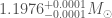 with the high-spin. This corresponds to a physical chirp mass of
  .
. , for the low-spin prior it is
  and for the high-spin prior it is
  .
. –
– and
and  –
–
 with the high-spin prior. Here, we quote maximum a posterior value and narrowest 68% intervals as opposed to the usual median and symmetric 90% credible interval. You might think its odd that the uncertainty is smaller when using the wider high-spin prior, but this is just another consequence of the difference in the inclination measurements. The values are largely in agreement with our initial values.
 . With the high-spin prior, we can only set an upper bound of
  . With the low-spin prior, we find that we are still consistent with zero deformation, but the distribution peaks away from zero. We have
  using the usual median and symmetric 90% credible interval, and
  if we take the narrowest 90% interval. This looks like we have detected matter effects, but since we’ve had to use the low-spin prior, which is only appropriate for neutron stars, this would be a circular argument. More details on what we can learn about tidal deformations and what neutron stars are made of, under the assumption that we do have neutron stars, are given in the
  of the coalescence time). We still don’t find anything, but now we set much tighter upper limits on what signal there could be there.
 ), as well as it being thermodynamically stable. Accommodating the most massive neutron star turns out to be an important piece of information.
 neutron star, these results indicate that the tidal deformation parameter would be
  . We favour softer equations of state over stiffer ones [
 must be greater than that for the smaller neutron star
  . The green shading and (50% and 90%) contours are calculated using the equation-of-state insensitive relations. The blue contours are for the parametrised equation-of-state model. The orange contours are from the
  ) neutron star is
 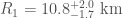 and the radius of the lighter (
 –
– ) neutron star is
  . With the parametrised equation-of-state model, the radii are
 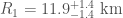 (
( ) and
) and  (
( –
–
 in radius. We now know that’s not the case.
 , which is basically all (99.996%) of them. Therefore, it’s unlikely that a cluster is the source of this binary.
 (3-sigma upper limit of
  ), towards the bottom end of our range, but their rate increases if not all mergers are as bright as AT 2017gfo.
 . They use to estimate the probability that AT 2017gfo and GW170817 are just a chance coincidence and are actually unrelated. The probability is
  at 90% confidence.
 , safely above our range.
 and
and  . Their figure 3 shows that this is well above expected rates.
 . That’s not too bad, but do stick with our result.
 ): LSST and WFIRST will see lots, about 7 and 8 per year respectively.
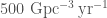 . They project that around 30% of gravitational-wave detections will be accompanied by gamma-ray bursts, once LIGO and Virgo reach design sensitivity.
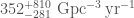 . To match up to our binary neutron star merger rate, we either need only a fraction of binary neutron star mergers to produce kilonova or for them to only be observable for viewing angles of less than
  . Their table 2 contains a nice compilation of rates for short gamma-ray bursts.

 after 67 days post-merger, but this evolves little over the duration of their observations (to day 152 post-merger), also suggesting a turn-over.
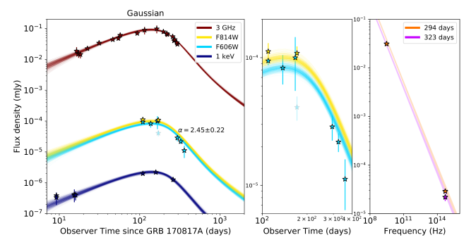
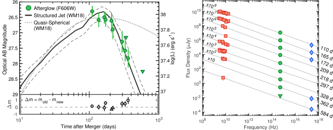


 .
. of the line of sight, and derive
  .
. using the Milky Way’s potential and
  using the Virgo cluster’s potential.
 , and that we are viewing it at an angle of
  . With X-ray and radio observations to 359 days,
  , and the width of a Gaussian structured jet would be
  . Using a combination of gravitational-wave, optical, radio and X-ray data,
  , for a Gaussian structured jet where they estimates the width
  . Using broadband synchrotron data to 800 days with a boosted fireball model,
  .
. , which (unsurprisingly) agrees pretty well with the result we obtained using the
  (where the errors are statistical uncertainty and an estimate of systematic error from calibration of the strain).
 (quoting median and 68% symmetric credible interval). Using different jet models changes their value for the Hubble constant a little; the choice of spin prior does not (since we get basically all of the inclination information from their radio observations). The results is still consistent with Planck and SH0ES, but is closer to the Planck value.
 . Combining this with results from the
  .
. , and hence
  .
. and a dark matter halo mass of
  , where we use the
  (but conclusions are similar using the
  . They also look at the star formation history, 90% were formed by
  ago, and the median mass-weighted stellar age is
  . From this they infer a merger delay time of
  −
− . From this, and assuming that the system was born close to its current location, they estimate that the supernova kick
  , towards the lower end of our estimate. They use
  .
. −
− and the mean stellar age is greater than about
  . They also give a luminosity distance estimate of
  , which overlaps with our gravitational-wave estimate. I’m not sure what value of
  they are using.
 . They find that 60% of stars by mass are older than
  and that less than 1% are less than
  old. Their Figure 5 has some information on likely supernova kicks, they conclude it was probably small, but don’t quantify this. They use
  .
. . They calculate a mass-weighted mean stellar age of
  and a likely minimum age for GW170817’s source system of
  . They use
  .
. , and suggest an old stellar population of age
  .
. and find a halo mass of
 and
and  ago.
ago. .
. . This implies a value for the Hubble constant of
  .
. . A neutron star would irradiate the ejecta with neutrinos, lower the neutron fraction and making the ejecta bluer. Since it is red, the neutrino flux must have been shut off, and the neutron star must have collapsed. We are in case b in their figure below.
 ). This is difficult to resolve unless neutron star radii are small (
 ).
).  –
– .
.  .
. has a radius of at least
  . They also estimate that the radius for the maximum mass nonrotating neutron star must be greater than
  .
.  , and for
  is greater than
  .
. ). They argue that the latter condition implies that the radius of a
  and the former that it is less than
  .
. . This is consistent with results in the
  .
. .
.
 inferred by


 –
– , whereas most of the radii inferred for GW170817’s components are larger. This paper argues that this can be resolved if one of the components of GW170817’s source was a hadron–quark hybrid star or a quark star.
 , which I think makes this an OK approximation;
  –
– .
. –
– and the radius in the range
  –
– .
. . These results are in good agreement with ours, their inclusion of electromagnetic data pushes their combined results towards larger values for the tidal deformation.
 –
– and the neutron star radius is
  –
– .
. .
. .
. (about 3%).
 .
.
