GW200115 and GW200105 are the first gravitational-wave candidates announced from the second half of LIGO and Virgo’s third observing run (O3b). They may be our first ever observations of neutron star–black hole binaries [bonus note]. These mixed binaries of one neutron star and one black hole have long proved elusive, but we are now on our way to revealing their secrets.
The population of compact objects (black holes and neutron stars) observed with gravitational waves and with electromagnetic astronomy, including a few that are uncertain. The sources for GW200115 (left) and GW200105 (right) are highlighted. Source: Northwestern
The first gravitational-wave signal ever detected, GW150914, came from a binary black hole system: two black holes that inspiralled together to form a bigger black hole. (I hope you are all imagining a bloopy chirp to accompany this). We had never before observed a binary black hole system. However, binary black holes have proved to be the most common source of gravitational waves, and we are now starting to understand their properties. We found our next type of gravitational-wave source with GW170817, which came from a binary neutron star system (two neutron stars that orbited each other). Before we had gravitational-wave astronomy, we knew this type of binary existed as we had observed pulsars in binaries thanks to radio astronomy. Yet, our second binary neutron star observation, GW190425, still showed that we didn’t know everything about their properties. After finding binary black holes and binary neutron stars, what about a mixed neutron star–black hole binary? These should exist, but finding evidence for them has proved difficult.
Time to tick neutron star–black hole binaries off the checklist. Part of a comic by Nutsinee Kijbunchoo drawn following the discovery of GW170817 showing Rai Weiss rather happy with his work. [Update]
Previous candidates
The first hints of neutron star–black hole binaries came in the first half of LIGO and Virgo’s third observing run (O3a, yes we are the best at thinking up names). The gravitational-wave candidate GW190426_152155 (the best at names) looks like it could have come from a neutron star–black hole binary. However, this is a quiet signal, so we are not sure whether it is real or a false alarm.
Our detection pipelines search the data from the detectors looking for signals. Our searches designed to specifically look for signals from binaries match the data against templates of what the signals should look like. From this comparison, they consider two pieces of information: how loud a signal is (its signal-to-noise ratio), and how consistent the signal is with the template. These are combined into a ranking statistic, and by comparing the ranking statistic with values produced by a background of noise, we can compute a false alarm rate of how often something at least this signal-like would happen in random noise. For GW190426_152155, this is , which isn’t too great.
The false alarm rate is not the end of the story though: we need to consider the true alarm rate: how often we expect to detect such a signal. If something is an everyday occurrence, you don’t need much evidence to convince yourself it’s real. Consider the quality of a photo you would need to convince yourself there was a horse walking around outside, and the quality needed to convince yourself there is a unicorn. For gravitational waves, a false alarm rate of would be enough to give you a fair (but not necessarily conclusive) probability of the signal being real if the source were a binary black hole, as we know they are pretty common. We don’t yet know how common gravitational waves from neutron star–black hole binaries are, but the fact that we are lacking good examples indicates that they are at least somewhat rare. Therefore, with the balance of probability, it seems plausible that GW190426_152155 is noise, and the hunt needs to continue.
Estimated total mass and mass ratio $q = m_2/m_1 \leq 1$ of the binary sources for the candidates in O3a. The contours mark the 90% credible regions. The dashed lines mark a robust upper limit on the maximum neutron star mass. Figure 6 of the GWTC-2 Paper.
The next potential candidate was GW190814. This is a super clear detection. However, the nature of the source is more mysterious. The primary (the more massive object in the binary) is definitely a black hole, but the secondary, at around (where is a solar mass) is either potentially too large to be a neutron star. We’re not entirely sure of the maximum mass a neutron star can be before collapsing. Hence, we’re not quite sure if we have a massive neutron star, or a really small black hole. I think the black hole is more likely. The curious nature of GW190814’s source means we are still missing an unambiguous neutron star–black hole.
Discovery
Observations in O3b changed everything. Within the space of ten days in January 2020 [bonus note], we collected two neutron star–black hole candidates: GW200105_162426 (GW200105 for short) and GW200115_042309 (GW200115).
GW200115 is a clear detection. All three detectors were observing at the time, and we get a good signal in both LIGO Livingston and LIGO Hanford (Virgo, being less sensitive currently, has less informative data). From these observations, our search algorithm GstLAL estimates a false alarm rate of , PyCBC estimates , and MBTA (being used for the first time for final search results) estimates . All of the search algorithms agree that this is a significant detection.
GW200105 is more difficult. LIGO Hanford was offline at the time, so we only have LIGO Livingston and Virgo. In Livingston data we can see a beautiful chirp, but in Virgo the signal is too quiet for the detection algorithms to use. This is like the case for GW190425, we must try to establish the significance using a single detector.
Time–frequency plots for GW200105 (left) and GW200115 (right) as measured by LIGO Hanford, LIGO Livingston and Virgo. LIGO Hanford was not observing at the time of GW200105. The chirp of a binary coalescence is clearest in Livingston for GW200105; these are usually hard to see for these types of signals. The Livingston data for GW200105 is shown after glitch subtraction, and the Livingston data for GW200115 shows light-scattering glitches at low frequencies. Figure 1 of the NSBH Discovery Paper.
When we have multiple detectors, we can ask how often we would expect to see the same signal at compatible times in multiple detectors. It is much less likely that multiple detectors would have the same random bit of noise in one detector and at the same time in another. We can estimate how often this would happen, for example, by comparing data from the detectors at different times. Considering many different time offsets, we can build up statistics for tens of thousands of years, even though we have only been observing for a few months (the upper limit on the false alarm rate quoted for GW200115 is because it stands out after we have exhausted all these times slides). When we have a single detector, we can’t do this.
GW200105 stands out from anything we have seen in the data we’ve analysed. We could therefore assign a false alarm rate of one per observing time. However, that doesn’t quite encode everything we know. We expect louder noise artifacts to be rarer than quieter ones. An outlier with signal-to-noise ratio of 12 should be rarer than one with signal-to-noise ratio of 11 (and GW200105 is over 13), and hence we can use this knowledge to try to extrapolate a false alarm rate.
Detection statistics for GW200105, GW200115 and GW190426_152155, showing they compare to background data. The plot shows the signal-to-noise ratio and signal-consistency statistic from the GstLAL algorithm. The coloured density plot shows the distribution of background triggers. LHO indicates a trigger from LIGO Hanford, and LLO indicates a trigger from LIGO Livingston. GW200105 is distinct from anything else seen in O3. However, GW200105 is calculated less significant than GW200115 as it only has a trigger from a single detector. Figure 3 of the NSBH Discovery Paper.
Currently, only GstLAL can calculate single-detector false alarm rates. PyCBC and MBTA both identify the same feature in the data, but cannot assign a significance to this. Using GstLAL’s extrapolation, which is chosen to be conservative (not as conservative as one per observing time, but a better representation of the data), we calculate a false alarm rate of . This is good enough to be interesting, and better than for GW190426_152155, but not enough to be absolutely conclusive. I think we may see some active development of estimating single-detector false alarm rates (or lowering the threshold for Virgo data to be used) in the future to try to address these difficulties.
It is very tempting to look at GW200105‘s clear chirp and convince yourself it must be real. However, our detection algorithms are more sensitive than our eyes and more reliable. They are carefully tested, and build up their statistics analysing large chunks of data. Hence, we should acknowledge that the difficulty in assigning a false alarm rate is an intrinsic difficulty when you only have so much data. Even the best signal can only end up with a modest false alarm rate. It’s kind of like winning the lottery on your third go if you don’t know how the lottery works: you can estimate that the probability of winning is about 1/3, even if you suspect it should be much smaller. The results computed for this paper only use a fraction of O3b, so we could be able to do a little better in the future.
Sources
Let us assume both signals are real, where do they come from? Do we at last have our undisputable neutron star–black hole binaries?
We infer [bonus note] that GW200115 comes from a binary with component masses and (or and if we restrict the secondary’s spin to ). The primary here looks to be a black hole. It is one of the smallest we have seen. The uncertainties on the measurement potentially take it into the hypothesised lower mass gap between neutron stars and black holes suggested from X-ray observations (and somewhat questioned by GW190814); however, there is a 70% chance that the mass is , so it is pretty consistent with the population of black holes we’ve seen in X-ray binaries. The secondary is perfectly in the neutron star range. Hence, this looks like a great neutron star–black hole binary candidate.
For GW200105, we infer that the primary has mass and secondary has mass (or and with low secondary spin). The primary is a nice black hole, the secondary is a nice plump neutron star. It is towards the more massive end of the distribution we have seen with radio observations, but it is consistent with past observations. Unlike for GW190814, we do not have any trouble explaining such as mass given what we know about the stiffness of neutron star stuff™. This is another good neutron star–black hole binary candidate.
Estimated masses for the binary primary and secondary masses and for neutron star–black hole binary candidates. The two-dimensional plot shows the 90% probability contour. For GW200105 and GW200115 we show results for two different spin priors for the secondary. The one-dimensional plot shows individual masses; the vertical lines mark 90% bounds away from equal mass. Estimates for the maximum neutron star mass (based upon Galactic neutron stars and studies of the equation of state) are shown for comparison with the mass of the secondary. Figure 4 of the NSBH Discovery Paper.
The masses for GW200115 overlap nicely with those inferred for GW190426_152155 and [bonus note]. The uncertainties for GW190426_152155 are larger, on account of it being quieter. Perhaps this could indicate this is fairly typical for neutron star–black hole binaries (and we might need to revise that true alarm rate)? It’s still too early to say, but I very much look forward to finding out!
The masses align nicely with expectations for neutron star–black hole binaries, so there are no surprises there. Ideally, we would confirm that we have seen neutron stars by measuring the tidal distortion of the neutron star [bonus note]. Unfortunately, these effects get harder to measure when the asymmetry in masses gets more significant, and we can’t pick anything out of the data. However, we did compare the secondary masses to various expectations for the maximum neutron star mass, and find that there’s over a 93% probability that the secondaries are safely below this. In conclusion, I think we have a good case for having completed our set of binaries and found neutron star–black hole binaries.
Estimated orientation and magnitude of the two component spins for GW200105 (left) and GW200115 (right). The distribution for the more massive primary component is on the left, and for the lighter secondary component on the right. The probability is binned into areas which have uniform prior probabilities, so if we had learnt nothing, the plot would be uniform. The maximum spin magnitude of 1 is appropriate for black holes. The solid line shows the 90% credible region using the high spin prior (which is used for the rest of the plot) and the dashed line shows the 90% contour for the low-spin prior. Figure 6 of the NSBH Discovery Paper.
The spins are more interesting. Spins range from zero for non-spinning, to one for a maximally spinning black hole. As a consequence of the large mass asymmetry, we measure the spin of the black holes better than for the neutron stars. For GW200105, we can constrain the spin magnitude to be at 90% probability (or with the low neutron star spin prior). This matches what we have seen for a lot of our black holes (as for GW190814‘s primary, but probably not for GW190412‘s primary), that their spins are small and nicely consistent with being zero.
For GW200115, the primary spin is also consistent with zero. However, there is also support for larger spins, and intriguingly, spin misaligned (or even antialigned as there’s little evidence of spin components in the orbital plane) with the orbital angular momentum. It is often convenient to work with the effective inspiral spin, which is a mass-weighted combination of the two spins projected along the direction of the orbital momentum. A positive value indicates the spins are overall aligned with the orbital angular momentum, while a negative value indicates the spins are overall misaligned. For GW200105, we find (or with low neutron star spin). This is consistent with zero, and what you would expect if spins were small, or if there were no preferred alignment. For GW200115 however, we find ( with low neutron star spin). This is still consistent with positive or zero values, but prefers negative values.
Generally aligned spins are expected for binaries formed from two binary stars that lived their lives together. The stars would have formed from the same cloud of gas, so you would expect the stars to start out rotating the same way. Tides and mass transfer between the stars should also help to align spins. Supernova explosions could tilt the spins, but it’s hard to get a complete reversal without disrupting the binary. This did happen for the double pulsar, so it’s not impossible, but overall you would expect it to be rare. However, for binaries formed dynamically, the spins would be randomly aligned.
Does the spin for GW200115 thus point to a dynamical origin? That would be unexpected, as isolated evolution generally predicts higher rates of forming neutron star–black hole binaries than dynamical channels. Dynamical channels tend to prefer making more massive binaries. The spin is perfectly consistent with being small and aligned, so perhaps that is the correct answer, and there’s nothing unexpected to see.
Estimated primary mass , spin component in the orbital plane , and spin component aligned with the orbital angular momentum and for GW200115. The (off-diagonal) two-dimensional plots show the correlations between parameters. The solid lines indicate 50% and 90% credible regions with the high-spin prior for the secondary, and the dashed lines show the same for the low-spin prior. The (on-diagonal) one-dimensional plots show probability densities. The vertical lines indicate 90% credible intervals. The black lines show the priors. Figure 7 of the NSBH Discovery Paper.
Since the spin is correlated with the mass, if we impose that GW200115‘s primary spin is small and aligned, we also find that the primary mass is towards the upper end of its range. This would keep it safely out of the proposed range of the lower mass gap. I’m not sure if that is of any physical relevance (as I’m not sure if I believe there is a gap), but it is potentially worth keeping in mind if you want to model the progenitor (you need to fit mass and spin together).
I look forward to lots of studies looking at how to form these systems.
Rates
Now we have confirmation that neutron star–black hole binaries exist, how many do we think there are out there? To go from our detections to a merger rate density, we need to assume something about the population of neutron star–black hole binaries (we need to know about the systems that we could have observed but didn’t). This is rather tricky, as neutron star–black hole binaries could potentially have a diverse range of properties, and we can’t be sure of this distribution with only a couple of observations. Therefore, we’ve tried a few different things.
First, we considered what are the rates of binaries that match the inferred properties of the two sources. We infer that the rate of GW200115-like binaries is using the results of GstLAL (and using PyCBC). The rate of GW200105-like binaries is (since PyCBC couldn’t detect this event, we could only set an upper limit, which is less interesting). GW200115 is less massive than GW200105, and so could not be detected to as great a distance. Therefore, since we’ve detected one of both, it means that the rate of GW200115-like binaries should be a bit higher. If we assume all neutron star–black hole binaries are like one of the two, we find an overall event-based rate of .
Probability distribution for the neutron star–black hole binary merger rate density. The green curve shows the event-based rate assuming all neutron star–black hole binaries are like GW200105 or GW200115. The black line assumes a broader population that also includes GW190814 and higher mass black holes. The vertical lines mark the 90% credible interval. Figure 9 of the NSBH Discovery Paper.
The second approach is to take a much more agnostic approach, and consider all output from our detection pipelines over a plausible mass range. The population here is defined more for convenience than anything else. We picked search triggers (down to a signal-to-noise ratio) corresponding to binaries with a primary mass between and and a secondary mass between and . The upper limit on the primary mass is set by the limits of our waveforms. Potentially, this mass could catch some binary neutron stars or binary black holes too. Therefore, we consider a mixture model and probabilistically assign candidates to being either noise, binary neutron star (if both components are below ), binary black hole (if both components are above ), and neutron star–black hole binaries (for things in between). I think we’ve been very inclusive in defining the neutron star–black hole space here, both excluding the possibility of binary neutron star components above (which I think unlikely, but possible), and binary black hole components below (which I think probable). Therefore, we should absolutely not be missing any neutron star–black holes (GW190814’s source is counted as a neutron star–black hole in this calculation). This rate comes out as .
I don’t think these will rule out any models, but they give the ballpark to aim for. As we find more neutron star–black hole candidates, these rates should evolve as our uncertainties will shrink, and we get a better understanding of the source population.
Predictions for the neutron star–black hole binary merger rate density as modelled by the COMPAS population synthesis code. The different models illustrate variations in the input physics, highlighting the range of predictions for isolated binary evolution. Other channels could potentially form neutron star–black hole binaries too. Figure 9 of Broekgaarden et al. (2021).
Summary
We have finally found our neutron star–black hole binaries. They’re pretty neat. These are the first discoveries from O3b. They will not be the last.
I like to think of neutron star–black hole binaries as the mirror counterparts of fluffernutter cookies. Black holes are black and super dense, completely unlike marshmallows. Neutron stars are made of something mysterious that we don’t know the properties of, but we think all neutron stars are made of the same type of stuff™, whereas peanut butter is made of well known ingredients, but has both smooth and crunchy equations of state. Despite the difference in ingredients, for both, when we mix the two types we get something delicious.
Even years
Previously, all our LIGO–Virgo discoveries came during odd-numbered years, so I was kind of hoping for a quiet 2020. This didn’t work out.
Waveform models
One of the most difficult things with inferring the properties of neutron star–black hole binaries is the waveform models that we use. We need accurate models to compare with the data to get good estimates of the parameters. Unfortunately, we don’t have models that include all the physics we want (spin precession, higher-order multipole moments, and the effects of the neutron star stuff™). From our tests, it seems like spin precession and higher-order multipole moments are more important. The latter is certainly important for asymmetric binaries. Therefore, for our main results, we use binary black hole waveforms that include spin precession and higher-order multipole moments (but no neutron star stuff™ effects). These models should be a pretty good representation of the overall physics (especially if the neutron tar gets swallowed whole). However, they may not give the best estimate of the final black hole mass. In the paper, we used the neutron star–black hole waveforms that include neutron star stuff™ effects but not spin precession and higher-order multipole moments, but I think it’s a bit confusing to mix the two results here, so I’ll skip over final masses and spins.
GW190426_152155’s properties
While GW190426_152155 agrees nicely with GW200115‘s masses, its other properties are somewhat different. Its effective inspiral spin is (compared with ), and its distance is . (compared with ). The sky positions are also not significantly overlapping.
Electromagnetic observations
An electromagnetic counterpart, as was found for GW170817, would confirm the presence of stuff™, and that we didn’t just have two black holes. However, with these mass black holes, we would expect the neutron stars to be pretty much swallowed whole (like me consuming a fluffernutter cookie) with nothing to see [bonus bonus note]. So far nothing has been reported, which is about as surprising as failing to find a needle in a haystack, when there is no needle.
Ejecta
We estimate that the amount of neutron star stuff ejected during the merger is less than . This is very small by astronomical standards, but is still pretty large. It’s around a third of the mass of the Earth, and would correspond to around 1,000,000,000,000,000,000,000 elephants. Sadly, it is not expected that material ejected from neutron stars would directly turn into elephants, and elephants do remain endangered.
GW190521 is a huge discovery—it a gravitational wave signal from the coalescence of two black holes to form one about (where our Sun has a mass of ). That is the largest black hole we have yet discovered with gravitational waves. It is the first definitive discovery of an intermediate-mass black hole. It is also a puzzle, as it is a mystery how its source could form…
How big can a black hole be?
Anything can become a black hole if it is squeezed enough [bonus note]: you just need to pack enough stuff into a small enough space (just like when taking a Ryanair flight). In practice, most stuff is stiff enough to push back against squeezing to avoid becoming a black hole. It’s only when you get the core of a star about somewhere between and that gravity becomes strong enough to collapse things down to a black hole [bonus note]. Above this threshold, can we have a black hole of any size?
The biggest black holes are found in the centres of galaxies. These can be hundreds of thousands to tens of billions the mass of our Sun. Our own Milky Way has a rather moderate black hole. These massive (or supermassive) black holes are far bigger than any star. Even Elvis. They therefore couldn’t have formed from a collapsing star. So how did they form? The truth is that we’re not sure. It’s possible that we started with smaller black holes and fed them up, or merged them together, or a mixture of both. These initial seed black holes could have formed from stars, or possibly giant clouds of collapsing gas (which may form black holes). In any case, whatever mechanism created these black holes needs to work quickly, as we know from observations of quasars, that there are massive black holes by the time the Universe is a mere billion years old. To figure out how massive black holes form, we need to discovery their seeds.
The shadow of a black hole reconstructed from the radio observations of the Event Horizon Telescope. The black hole lies at the centre of M87, and is about . Credit: Event Horizon Team
Between stellar-mass black holes and massive black holes should lie intermediate-mass black holes. These are typically defined as having masses between and . Massive black holes should grow from these smaller black holes. However, we have never found one, they are the missing link in the black hole spectrum. There are candidates: ultrabright X-ray sources, or globular clusters with suspiciously moving stars, but none of these is rock solid, and couldn’t be explained another way. GW190521 changes this, at the merger remnant is without doubt an intermediate-mass black hole.
This discovery shows that intermediate-mass black holes can form from mergers of smaller black holes. However, this doesn’t yet solve the mystery of how massive black holes are grown; we need observations of larger intermediate-mass black holes for that. We’ll keep searching.
What I find more exciting about GW190521 are the masses of the two black holes that merged. Our analysis gives these as and . The large black hole masses extremely difficult to explain.
Estimated masses for the two components in the binary . We show results several different waveform models and use the numerical relativity surrogate (NRSur PHM) as our best results. The two-dimensional shows the 90% probability contour. The dotted lines in one-dimensional plots the symmetric 90% credible interval. Part of Figure 1 of the GW190521 Implications Paper.
When you form a black hole from a star, its mass depends upon the mass of of its parent star. More massive stars generally form bigger black holes, but because of all the physics that goes on inside stars, it’s not a simple relationship. One important phenomena in determining the fate of massive stars is pair instability. When the cores of stars become very hot (, just slightly less than the temperature of the mozerlla on that first bite of pizza, even though you should know better by now), the photons of light (gamma-rays) bouncing around inside the core become energetic enough to produce pairs of electrons and positrons [bonus note]. For the star, this causes some trouble. Its core is mostly supported by radiation pressure. If photons start disappearing as they are converted to electrons and positrons, then there isn’t as much radiation around, and the star will start to collapse. As it collapses, explosive nuclear reactions are triggered. Pair instability kicks in for stars with helium cores about . If the core is between and about , the star will blast off its outer layers, possibly repeating the cycle of pair-instability collapse and explosion many times. This results in smaller black holes than you might otherwise expect. For helium cores between and about , the explosion completely destroys the star, leaving nothing behind. These stars never collapse down to a black hole, and this leaves a gap, predicted to start somewhere between and .
Remnant (white dwarf, neutron star or black hole) mass for different initial (zero age main sequence) stellar masses . This is just for single stars, and ignores all the complicated things that can happen in binaries. The different coloured lines indicate different metallicities (higher metallicity stars lose more mass through stellar winds). The two panels are for two different supernova models. The grey bars indicate potential mass gaps: the lower core collapse mass gap (only predicted by the Rapid model) and the upper pair-instability mass gap. The tick marks in the middle are various claimed gravitational-wave source, colour-coded by the total mass of the binary . Figure 1 of Zevin et al. (2020).
The more massive of GW190521’s black holes sits squarely in the expected pair-instability mass gap. How can we form such a system?
To delve into all the details, we have put together two papers on GW190521. The high mass of the system poses challenges not just for our understanding of astrophysics, but also for our data analysis. Below, I’ll go through what we have discovered.
The signal
GW190521 was first identified in our online searches about 20 seconds after we took the data. All three of our detectors were online and observing at the time. It was a short bleep of a signal indicating a high mass system. Short signals always make me suspicious as they can easily confused with some types of glitch. The signal was picked up by multiple search algorithms, which generally is a good sign, as they all estimate the background of noise in a slightly different way. However, the estimated false alarm rates were only one per few years. That’s not terribly impressive—it’s the range where things can change as we collect more data. Immediately, checks of the signal began. We have many ways of monitoring our detectors, and experts started running through these. Microphones at Hanford picked up a helicopter overhead a few minutes later, but that’s too far away in time to be related to the signal. The initial checks all looked OK, so we were confident that it was safe to share the candidate detection S190521g.
Visualisations of GW190521. The top panels show whitened data and reconstructed waveforms from the template-free detection algorithm cWB, BayesWave (which reconstructs the signal from sine–Gaussian wavelets), and our parameter estimation code LALInference (which uses binary black hole waveforms). The bottom panels show time–frequency plots: each plot has a different scale as the signal is loudest in LIGO Livingston and hardly noticeable in Virgo. As the signal is so short, we don’t see the usual chirp of a binary coalescence clearly. Figure 1 of the GW190521 Discovery Paper.
After hearing that the initial checks were complete, I went to bed, little knowing the significance of what we had found. The initial estimates for the masses of a binary come from our search pipelines—specifically the pipelines that match signal templates to the data. At high masses, the search template bank doesn’t have many templates, so the best fitting template can be quite a way from the true value. It was only after completing a proper parameter estimation analysis that we get a good idea of the masses and their uncertainties. When these results came in we found that we potentially had something lying smack in the middle of the pair-instability mass gap. That was, if the signal were real.
While initial checks of the signal showed nothing suspicious, we always do more offline checks. For GW190521 there were a few questions that took some digging to understand.
First, the peak of the signal is around 60 Hz. This is also the mains frequency in the US, so there was concern that the signal was contaminated by noise caused by this (which would obviously be shocking). A variety of careful investigations were done subtracting out noise from the mains. In the end, it turns out that this makes negligible difference to the results, which is nice.
Second, there was concern over the shape of the signal. Our template-based search algorithms always look at how well the signal matches the template: if you get a really good match in one frequency range, but not another, then that’s an indicator that you have some random noise rather than a true signal. This consistency test is summarised in a statistic, which should be around 1 if all is OK, and larger if things don’t fit. For the PyCBC algorithm, the value for the Livingston data was about 3. Since the signal was loudest in Livingston, was this cause for alarm? One explanation could be that the template wasn’t a good fit because the templates used by the search don’t include the effects of spin precession. Hence, if you have a signal where spin precession is important, you would expect a bad fit. Checking the consistency with templates which included precession did give better consistency. However, the GstLAL algorithm also used templates without precession, and its consistency test looked fine. Therefore, it couldn’t just be precession. It seems that the key is that there are so few templates in the relevant area for PyCBC’s template bank (GstLAL had things better covered). Hence, it is hard to find a good fitting template. Adding the best fitting template from the GstLAL bank to the PyCBC search leads to it being picked out as the best template too, with a consistency check statistic of 1.7 (not perfect, but not suspicious). I think this highlights the importance of not limiting yourself to only finding what you expect: we need to include the potential for our searches to discover things outside of what we have discovered in the past.
Finally, there was the difference in significance reported by the different search algorithms. In addition to the template-based searches, we also have searches which look for more generic signals without templates [bonus note], instead using the consistency in the data from different detectors to spot signals. Famously, our non-template algorithm coherent WaveBurst (cWB) made the first detection of GW150914 (other algorithms weren’t up-and-running at the time). Usually, the template searches should do better as they know what they are looking for. This has mostly been the case so far. The exception was GW170729, our previously most massive and lowest significance detection. Generally, you expect searches to disagree more on quiet signals (not too much of an issue for GW190521), as then how they characterise the noise background is more important. We also expect the template searches to lose their advantage for very short signals, when there’s not much for a template to match, and when the coherence check used by cWB comes in especially handy. GW190521 is again found with greatest significance by cWB. In our final searches (using all the data from the first six months of the third observing run), cWB gives a false alarm rate of 1 per 4900 years (pretty darn good—at least a Jammie Wagon Wheel in biscuit terms), GstLAL gives 1 per 829 years (nice—a couple of Fruit Creme biscuits), and PyCBC gives 1 per 0.94 years (not at all exciting—an Iced Gem at best). Should we be suspicious of the difference? Perhaps cWB can pick up on something extra in the signal because actually the source isn’t a quasicircular binary [bonus note] as assumed by our templates? We know that the search templates are missing some features, like the effects of spin precession, and also higher order multipole moments. Seeing how our search algorithms cope finding simulated signals that include these extra bits of physics, we find that similar discrepancies between cWB and GstLAL happen around 8% of the time, while for cWB and PyCBC they happen about 3% of the time. That’s enough to make me go Hmm, but not enough to convince me that we’ve detected a completely new type of signal, one which doesn’t come from a quasicircular binary.
The conclusion from our analysis is that GW190521 is a good-looking gravitational wave signal. We are confident that it is a real detection, even though it is really short. However, we can’t be positive that the source is quasicircular binary. That’s the most likely explanation, and consistent with what we’ve seen, but potentially not the only explanation.
There are other sources for gravitational waves beyond quasicircular binaries. One of the best known would be a supernova explosion. GW190521 is certainly not one of these. For one thing, the signals are much longer and more complicated, and for another, we could really only detect a supernova within our own galaxy, and we probably would have noticed that happen. Another hypothesised search which could produce a nice, short bleep of a signal would be a cosmic string. Vibrations or ripples along a cosmic string can source gravitational waves, and while we don’t know if cosmic strings exist, we do have templates for what these signals should look like. Using these, we can compare how well the data are described by cosmic string signals compared to our quasiciruclar binary templates. We find Bayes factors of about in favour of the binary signals, so it’s probably not cosmic strings. Finally, you’ve perhaps noticed that I’ve been writing quasicircular [bonus note] a lot. Part of that is because it’s a cool word (25 points in Scrabble), but also because it’s possible that we have an eccentric binary. These are difficult to model, so we don’t have lots of good templates for them, but when you have a short signal, it is possible that eccentricity could be confused with spin precession. This would lead us to overestimating the distance and underestimating the masses. Initial studies do seem to show that an eccentric signal fits the data well (Romero-Shaw et al. 2020; Gayathri et al. 2020). An eccentric binary is the most probable alternative to a quasicircular binary, but it is pretty improbable. Since eccentricity is lost during inspiral, we would need something to have pumped the eccentricity, which is difficult for a binary so close to merger. I would bet my Oreos on the source being a quasicircular binary.
The source properties
If we stick with the assumption of a quasicircular binary, what can we tell about the source? We have already covered the component masses of and , and that the merger remnant is . The plot below shows the final mass as well as the spin, which is . For the black holes formed from the mergers of near equal mass binaries, you’d expect the final spin to be around .
Estimated mass and spin for the final black hole. We show results several different waveform models and use the numerical relativity surrogate (NRSur PHM) as our best results. The two-dimensional shows the 90% probability contour. The dotted lines in one-dimensional plots the symmetric 90% credible interval. The mass is safely above the conventional lower limit to be considered an intermediate-mass black hole. Figure 3 of the GW190521 Implications Paper.
We can also get an estimate of the final spin from the final part of the signal, the ringdown. This is where the black hole settles down to its final state, like me after 6 pm. What is neat about using the ringdown is that we don’t need to assume that the binary was quasicircular, as we only care about the black hole formed at the end. The downside is that we don’t get an estimate of the distance, so we only measure the redshifted final mass . Looking at the ringdown, we get lovely consistent results trying ringdown models at different start times and including different higher order multipole moments, and all agree with the analysis of the entire signal using the quasicircular templates.
Estimated redshifted mass and spin for the final black hole. We show results several different insprial–merger–ringdown waveform models, which we use for our standard analysis, as well as ringdown-only waveforms. They agree nicely. The two-dimensional shows the 90% probability contour. The dotted lines in one-dimensional plots the symmetric 90% credible interval. The mass is safely above the conventional lower limit to be considered an intermediate-mass black hole. Part of Figure 9 of the GW190521 Implications Paper.
Being able to measure the ringdown at all is an achievement. It’s only possible for loud signals from high mass systems. The consistency of the mass and spin estimates is not only a check of the quasicircular analysis. It is much more powerful than that. The ringdown measurements are a test of the black hole nature of the final object. All looks as expected so far. I really want to do this for louder signals in the future.
Returning to the initial binary, what can we say about the spins of the initial black holes? Not much, as it is difficult to extract information from such a short waveform.
The spin components aligned with the orbital angular momentum affect the transition from inspiral, and have a small influence on the final spin. We often quantify the aligned components of the spin in the mass-weighted effective inspiral spin parameter, which goes from for both the spins being maximal and antialigned with the orbital angular momentum to for both spins being maximal and aligned with the orbital angular momentum. We find that , consistent with no spin, spins antialigned with each other or in the orbital plane. The result is strongly influenced by the assumed prior, we’ve not learnt much from the signal.
The component of the spin in the orbital plane (perpendicular to the orbital angular momentum) control the amount of spin precession. We often quantify this using the effective precession spin parameter , which goes from for no in-plane spin, to for maximal precession. Precession normally shows up in the modulation of the inspiral signal, so you wouldn’t expect to measure it well from a short signal. However, it can also influence to amplitude of the signal around merger, and we seem to get a bit of information here, which seems to prefer larger . We find , but there’s support across the entire range.
Estimated effective inspiral spin and effective precession spin . We show results several different waveform models and use the numerical relativity surrogate (NRSur PHM) as our best results. The two-dimensional shows the 90% probability contour. The dotted lines in one-dimensional plots the symmetric 90% credible interval. We also show the prior distributions in the one-dimensional plots. Part of Figure 1 of the GW190521 Implications Paper.
Looking at the spins overall, the lack of aligned spin plus the support for in-plane spins means that we prefer misaligned spins. You wouldn’t expect this for two stars which have lived their lives together as a binary, but it wouldn’t be implausible for a dynamically formed binary. A dynamical formation seems plausible to me, but since the spin measurements aren’t too concrete, we can’t really rule too much out [bonus note].
Finally, let’s take a look at the distance to the source. Our analysis gives a luminosity distance of . This makes the source a good contender for the most distant gravitational wave source ever found [bonus note]. It’s actually far enough, that we might want to reconsider our standard approximation that sources are uniformly distributed like . This would be OK if sources were uniformly distributed in a non-evolving Universe, but sadly we don’t live in such a thing, and we have to take into account the expansion of the Universe, and the evolution of the galaxies and stars within it. We’ll come back to look at this when we present our catalogue of detections from the first part of the third observing run.
The astrophysics
Exploring the upper mass gap
The location of the upper mass gap is pretty well determined. There are a variety of uncertainties in the input physics, such as the nuclear reaction rate for burning carbon into oxygen, the treatment of convection inside stars or if stars rapidly rotate which can alter the cut-off. No-one has tried varying all these together, but individually you can’t get above about for your black hole. Allowing for new types of particles (like axions, one of the candidates for dark matter, and possibly the explanation for why teenage boys can smell terrible) can potentially increase the limit to above , but that is extremely speculative (I’d love it if it were true). Sticking to known physics, at face value, it is hard to explain the mass of the primary black hole from our understanding of how stars evolve.
There are potentially ways around the mass gap with help from a star’s environment:
Super efficient accretion from a companion star can grow black holes into the mass gap. Then you wouldn’t expect the total mass of the binary to over about , so we’d need to swap out partners in this case.
The pair instability originates in the helium core of a star. If we can find a way to grow the envelope of the star, while keeping the core below the threshold for the instability to set in, then the whole thing could collapse down to a mass gap black hole. This could potentially happen if two stars collide after one has already formed its helium core. The other gets disrupted and swells the envelope. This might be expected in stellar clusters. Similarly, a couple of recent papers (Farrell et al. 2020; Kinugawa, Nakamura & Nakano 2020) have also suggested that the first generation of stars, which have few elements other than hydrogen or helium, could also collapse down to black holes in this mass range. The idea here is that these stars lose much less of their envelopes due to stellar winds, so you can end up with what we would otherwise consider an oversized envelope around a core below the pair instability threshold
We could have two black holes merge to form a bigger one, and then have the remnant go on to form a new binary. You would need a dense environment for this, somewhere like a globular cluster where it’s easy to find new partners. Ideally, somewhere with a large escape velocity, perhaps a nuclear star cluster, which has a high escape velocity so that it is more difficult for the remnant black hole to get kicked out at any point: gravitational waves give a recoil kick, and close encounters with other objects can also lead to the initial binary getting a kick.
Especially good for growing black holes may be if they are embedded in the accretion disc around a supermassive black hole. Then these disc black holes can merge with each other whilst being unlikely to escape the environment. Additionally, they can swallow lots of gas from the surrounding disc to help them grow big and strong.
There is also the potential that we don’t have a black hole formed from stellar collapse, but instead a primordial black hole formed from dense regions in the early Universe. These primordial black holes are a another candidate for dark matter. I like that there are two options for potential dark matter-related formation channels. It’s good to have options.
The difficulty with all of these alternative formation channels is matching the observed rate for GW190521-like systems. It’s not enough for a proposed channel to be able to explain the system’s properties, it also needs to make enough of them for us to have come across one. From our data, we infer that GW190521-like systems have a merger rate density of . Predicted rates for the various formation mechanisms discussed above can be rather uncertain (kind of like how the exact value of a small bag full of Bitcoin is uncertain), so I would like to see more work on this, before picking a most plausible option.
Hierarchical mergers
We did do some quantitative analysis for the case of hierarchical mergers of black holes, following the framework outlined in Kimball et al. (2020). This simultaneously fits the mass and spin distribution for the first generation (1g) of black holes formed from stars, and a fraction of hierarchical mergers involving second generation (2g) merger remnants. To calibrate the number of hierarchical mergers, we use globular cluster simulations.
Using our base model, where the 1g+1g population is basically the Model C we used to describe our detections from the first two observing runs, we find that the odds are in favour of GW190521 being a 1g+1g merger. Hierarchical mergers are so rare, that it’s actually more probable that we squish down the inferred masses and have something from the tail of the 1g population.
The rate of hierarchical mergers, however, is very sensitive to the distribution of spins of 1g black holes. Larger spins give bigger kicks (even a spin of 0.1 is enough to mean remnants are hardly ever retained in typical globular clusters). If we add into the mix a fraction of 1g+1g binaries which have 0 spin (motivated by recent simulations), we improve the odds to be roughly even 1g+1g vs 1g+2g, and less common for 2g+2g. Given that we are not taken into account that only a fraction of binaries would be in clusters, which would reduce the odds of a hierarchical merger considerably, this isn’t quite enough to convince me.
However, what if we were to turn up the mass of the cluster? For our globular cluster model, we used , what if we tried , more like you would expect for a nuclear star cluster? We shouldn’t really be doing this, as our model is calibrated against globular cluster simulations, and nuclear star clusters have different dynamics, but we can use our results as illustrative. In this case, we find odds of about 1000:1 in favour of hierarchical mergers. This suggests that this option may be a promising one to follow, but we must moderate our results remembering that only a fraction of binaries would form in these dense environments.
The analysis is done using only our first 10 detected binary black hole from our first two observing runs plus GW190521. GW190521 is not the most representative of the third observing run detections (hence why it gets special papers™), so it is not exactly fair to stick it in to the mix to infer the population parameters. We’ll need to redo this analysis when we have the full results of the run to update the results. Having more binaries in the analysis should allow us to more precisely measure the population parameters, so we will be more confident in our results.
The surprise
After all our investigations, we thought we had examined every aspect of GW190521. However, there’s always one more thing. As we were finishing up the paper, a potential electromagnetic counterpart was announced.
Electromagnetic counterparts are not expected when two black holes merge—black holes are indeed black—however, material around the binary could produce light.
The counterpart was found by the Zwicky Transient Factory. They targeted active galactic nuclei to look for counterparts. These are the bright cores of galaxies where the supermassive black hole is feeding off a surrounding disc. In this case, they hypothesis that the binary had some gas orbiting around it, and when the binary merged, the gravitational wave recoil kick sent the remnant black hole and its orbiting material into the disc of the supermassive black hole. As the orbiting material crashes into the disc it will emit light. Then, once it is blasted away, material from the disc accreting onto the remnant black hole will also emit light. This seems to fit with what was observed, with the later powering the observed emission.
What I think is exciting about this proposal is that active galactic nuclei are one of the channels predicted to produce binaries as massive as GW190521! Therefore, things seem to line up nicely.
The three dimensional localisation for GW190521. The lines indicate the position of the claimed electromagnetic counterpart from around an active galactic nucleus. This location lies at the 70% credible level. Credit: Will Farr
What I think is less certain is if the counterpart is really associated with our gravitational wave source. The observing team estimate that the probability of a chance association is small. However, there is a lot of uncertainty in how active galactic nuclei can flare. The good news is that the remnant black hole may continue to orbit and hit the disc again, leading to another flare. The bad news is that the uncertainty on when this happens is many years, so we don’t know when to look.
Follow-up analyses by Ashton et al. (2020) and Palmese et al. (2021) cast the association as more uncertain. It is difficult to be confident of an association when the localization volume is so large. If we knew that this type of flare had to look exactly like the observed emission, that would help, but we can’t be that certain yet.
Overall, I think we need to observe another similar association before we can be certain what’s going on. I really hope this candidate counterpart encourages people to follow up more binary black holes to look for emission. The unexpected discoveries are often the most rewarding.
This is the paper announcing the gravitational wave detection. It follows our now standard pattern for a detection paper of discussing our instruments and data quality; our detection algorithms and the statistical significance of the search; the inferred properties of the source, and a bit of testing gravity; a check of the reconstruction of the waveform, and then a nice summary looking forward to more discoveries to come.
What is a little different for this paper is that because the signal is so short, we have had to be extra careful in our checks of the detectors’ statuses, the reliability of our detection algorithms, and the assumptions that go into estimating the source properties. If you are sceptical of being able to detect such short signals, I recommend checking out the Supplemental Material for a summary of some of the tests we did.
The GW190521 Implications Paper
Title: Properties and astrophysical implications of the 150 solar mass binary black hole merger GW190521
Journal:Astrophysical JournalLetters; 900(1):L13(27) arXiv:2009.01190 [astro-ph.HE]
Read this if: You want to understand the implications for fundamental physics and astrophysics of the discovery
In this paper we explore the properties of GW190521. We check the robustness of the inferred source properties. For such a short signal, our usual assumption that we have a quasicircular binary is probably the most sensible thing to do, but we can’t be certain, and if this assumption is wrong, then we will have got the properties wrong. Astronomy is hard sometimes. Assuming that our estimates of the properties are correct, we look at potential formation mechanisms. We don’t come to any firm conclusions, but sketch out some of the possibilities. We also look at tests of the black hole nature of the final object in a bit more detail. A few wibbles can sure cause a lot of excitement.
The uncertainty in when gravity will take over and squish things down to a black hole is set by the stiffness of neutron star matter. Neutron stars are the densest matter can be, this is the stiffest form of matter, the one most resistant to being crushed down into a black hole. The amount of weight neutron star matter can support is uncertain, so we don’t quite know their maximum mass yet. This made the discovery of GW190814 particularly intriguing. This gravitational wave came from a binary where the less massive component was about , exactly in the range where we’d expect the transition between neutron stars and black holes. We can’t tell for certain which it is, but I’ve bet my M&Ms on a black hole.
It’s potentially possible that there are black holes smaller than the maximum neutron star mass which didn’t form from collapsing stars. These are primordial black holes, which formed from overdense regions in the early universe. We don’t know for certain if they do exist, but we are looking.
Positrons
Positrons are antielectrons, the antimatter equivalent of electrons. This means that they share identical properties to electrons except that they have opposite charge. Electrons things that the glass is half-empty, positrons think it is half-full. Neutrinos think that the glass is twice as big as it needs to be, but so long as we have a well-mixed cocktail, who cares?
Burst searches
In the jargon of LIGO and Virgo, we refer to the non-template detection algorithms as Burst searches, as they are good at spotting bursts of gravitational waves. Burst is not a terribly useful description if you’ve not met it before, so we generally try to avoid this in our papers. A common description is an unmodelled search, to distinguish from the template-based searches which use model waveforms as input. However, it’s not really true that the Burst searches don’t make modelling assumptions about the signal. For example, the cWB algorithm used to look for binaries assumes that the frequency will increase with time (as you would expect for an inspiralling binary). To avoid this, we’ve sometimes describes the search algorithm as weakly modelled, but that’s perhaps no clearer than Burst. For this post, I’ll stick to non-template as a description.
Quasicircular
When talking about the orbits of binaries, we might be interested in their eccentricity. Eccentricity is a key tracer of how the binary formed. As binaries emit gravitational waves, they quickly lose their eccentricity, so in general we don’t expect there to be significant eccentricity for the binaries detected by LIGO and Virgo.
An orbit with zero eccentricity should be circular. However, since we have a binary emitting gravitational waves the orbit will be shrinking. As we have an inspiral, if you were to trace out the orbit, it would not be a circle, even though we would describe it as having zero eccentricity. This is particularly noticeable at the end of the inspiral, when we get close to the two objects plunging together. Hence, we describe orbits as quasicircular, which I think sounds rather cute.
The simulation above shows the orbit of an inspiral. Here the spins of the black holes also lead to the precession of the orbit, making it a bit more complicated than you might expect for a something described as circular, but, of course, not at all unexpected for something with a cool name like quasicircular. I also really like how this visualisation shows the event horizons of the two black holes merging.
Spin Bayes factors
To try to quantify the support for spin, we quote two Bayes factors. The first is for spin verses no spin. There we find a Bayes factor of about 8.3 in favour of there being spin. That’s not something you’d want to bet against, but for comparison, for GW190412 we found that is it over 400, and for GW151226 it is over a million. I’d expect any statement on spins for GW190521 will depend upon your prior assumptions. The second Bayes factor is in favour of measurable precession. This is not the same as comparing the Bayes factor between perfectly aligned spins (when there would be no precession) and generic, isotropically distributed spins. Instead we are comparing the scenario where we can measure in-plane spins verses the case where there are isotropically distributed but the in-plane spins don’t have any discernible consequences. Here we find a Bayes factor of 11.5 in favour of measurable precession. This makes sense as we do have some information on , and would expect an even Bayes factor of 1 if we only got the prior back. It seems we have gained some information about the spins from the signal.
For more on Bayes factors, I would suggest reading Zevin et al. (2020). In particular, this explains why it can make sense here that the Bayes factor for measurable precession is larger than the Bayes factor for there being spin. At first, it might appear odd that we can be more definite that there is precession than any spin at all. However, this is because in comparing spin verses no spin we are hit by the Occam factor—we are adding extra parameters to our model, and we are penalised for this. If the effects of spins are small, so that they are not worth including, we would expect no-spin to win. When looking at the measurability of precession, we have set up the comparison so that there is no Occam factor. We can only win, if waveforms with precession clearly fit the data better, or break even if they make no difference.
Economically large
To put a luminosity distance of in context, if you put $1 in a jar ever two weeks over the duration the gravitational wave signal was travelling from its source to us (7.1 billion years, about 1.5 times the age of the Sun), you would end up with about a net worth only 7% less than Jeff Bezos (currently $199.3 billion).
GW190814 is an exception discovery from the third observing run (O3) of the LIGO and Virgo gravitational wave detectors. The signal came from the coalescence of a binary made up of a component about 23 times the mass of our Sun (solar masses) and one about 2.6 solar masses. The more massive component would be a black hole, similar to past discoveries. The less massive component, however, we’re not sure about. This is a mass range where observations have been lacking. It could be a neutron star. In this case, GW190814 would be the first time we have seen a neutron star–black hole binary. This could also be the most massive neutron star ever found, certainly the most massive in a compact-object (black hole or neutron star) binary. Alternatively, it could be a black hole, in which case it would be the smallest black hole ever found. We have discovered something special, we’re just not sure exactly what…
The population of compact objects (black holes and neutron stars) observed with gravitational waves and with electromagnetic astronomy, including a few which are uncertain. GW190814 is highlighted. It is not clear if its lighter component is a black hole or neutron star. Source: Northwestern
Detection
14 August 2019 marked the second birthday of GW170814—the first gravitational wave we clearly detected using all three of our detectors. As a present, we got an even more exciting detection.
I was at the MESA Summer School at the time [bonus advertisement], learning how to model stars. My student Chase come over excitedly as soon as he saw the alert. We snuck a look at the data in a private corner of the class. GW190814 (then simply known as candidate S190814bv) was a beautifully clear chirp. You shouldn’t assess how plausible a candidate signal is by eye (that’s why we spent years building detection algorithms [bonus note]), but GW190814 was a clear slam dunk that hit it out of the park straight into the bullseye. Check mate!
Time–frequency plots for GW190814 as measured by LIGO Hanford, LIGO Livingston and Virgo. The chirp of a binary coalescence is clearest in Livingston. For long signals, like GW190814, it is usually hard to pick out the chirp by eye. Figure 1 of the GW190814 Discovery Paper.
Unlike GW170814, however, it seemed that we only had two detectors observing. LIGO Hanford was undergoing maintenance (the same procedure as when GW170608 occurred). However, after some quick checks, it was established that the Hanford data was actually good to use—the detectors had been left alone in the 5 minutes around the signal (phew), so the data were clean (wooh)! We had another three-detector detection.
The big difference that having three detectors make is a much better localization of the source. For GW190814 we get a beautifully tight localization. This was exciting, as GW190814 could be a neutron star–black hole. The initial source classification (which is always pretty uncertain as it’s done before we have detailed analysis) went back and forth between being a binary black hole with one component in the the 3–5 solar mass range, and a neutron star–black hole (which means the less massive component is below 3 solar masses, not necessarily a neutron star). Neutron star–black hole mergers may potentially have an electromagnetic counterparts which can be found by telescopes. Not all neutron star–black hole binaries will have counterparts as sometimes, when the black hole is much bigger than the neutron star, it will be swallowed whole. Even if there is a counterpart, it may be too faint to see (we expect this to be increasingly common as our detectors detect gravitational waves from more distance sources). GW190814’s source is about 240 Mpc away (six times the distance of GW170817, meaning any light emitted would be about 36 times fainter) [bonus note]. Many teams searched for counterparts, but none have been reported. Despite the excellent localization, we have no multimessenger counterpart this time.
Sky localizations for GW190814’s source. The blue dashed contour shows the preliminary localization using only LIGO Livingston and Virgo data, and the solid orange shows the preliminary localization adding in Hanford data. The dashed green contour shows and updated localization used by many for their follow-up studies. The solid purple contour shows our final result, which has an area of just . All contours are for 90% probabilities. Figure 2 of the GW190814 Discovery Paper.
The sky localisation for GW190814 demonstrates nicely how localization works for gravitational-wave sources. We get most of our information from the delay time between the signal reaching the different detectors. With a two-detector network, a single time delay corresponds to a ring on the sky. We kind of see this with the blue dashed localization above, which was the initial result using just LIGO Livingston and Virgo data. There are actual arcs corresponding to two different time delays. This is because the signal is quiet in Virgo, and so we don’t get an absolute lock on the arrival time: if you shift the signal so it’s one cycle different, it still matches pretty well, so we get two possibilities. The arcs aren’t full circles because information on the phase of the signals, and the relative amplitudes (since detectors are not uniformal sensitive in all directions) add extra information. Adding in LIGO Hanford data gives us more information on the timing. The Hanford–Livingston circle of constant time delay slices through the Livingston–Virgo one, leaving us with just the two overlapping islands as possibilities. The sky localizations shifted a little bit as we refined the analysis, but remained pretty consistent.
Whodunnit?
From the gravitational wave signal we inferred that GW190814 came from a binary with masses solar masses (quoting the 90% range for parameters), and the other solar masses. This is remarkable for two reasons: first, the lower mass object is right in the range where we might hit the maximum mass of a neutron star, and second, this is the most asymmetric masses from any of our gravitational wave sources.
Estimated masses for the two components in the binary . We show results several different waveform models (which include spin precession and higher order multiple moments). The two-dimensional shows the 90% probability contour. The one-dimensional plot shows individual masses; the dotted lines mark 90% bounds away from equal mass. Estimates for the maximum neutron star mass are shown for comparison with the mass of the lighter component . Figure 3 of the GW190814 Discovery Paper.
Neutron star or black hole?
Neutron stars are massive balls of stuff™. They are made of matter in its most squished form. A neutron star about 1.4 solar masses would have a radius of only about 12 kilometres. For comparison, that’s roughly the same as trying to fit the mass of M&Ms (plain; for peanut butter it would be different, and of course, more delicious) into the volume of just M&Ms (ignoring the fact that you can’t perfectly pack them)! Neutron stars are about times more dense than M&Ms. As you make neutron stars heavier, their gravity gets stronger until at some point the strange stuff™ they are made of can’t take the pressure. At this point the neutron star will collapse down to a black hole. Since we don’t know the properties of neutron star stuff™ we don’t know the maximum mass of a neutron star.
We have observed neutron stars of a range of masses. The recently discovered pulsar J0740+6620 may be around 2.1 solar masses, and potentially pulsar J1748−2021B may be around 2.7 solar masses (although that measurement is more uncertain as it requires some strong assumptions about the pulsar’s orbit and its companion star). Using observations of GW170817, estimates have been made that the maximum neutron star mass should be below 2.2 or 2.3 solar masses; using late-time observations of short gamma-ray bursts (assuming that they all come from binary neutron star mergers) indicates an upper limit of 2.4 solar masses, and looking at the observed population of neutron stars, it could be anywhere between 2 and 3 solar masses. About 3 solar masses is a safe upper limit, as it’s not possible to make stuff™ stiff enough to withstand more pressure than that.
At about 2.6 solar masses, it’s not too much of a stretch to believe that the less massive component is a neutron star. In this case, we have learnt something valuable about the properties of neutron star stuff™. Assuming that we have a neutron star, we can infer the properties of neutron star stuff™. We find that a typical neutron star 1.4 solar masses, the radius would be and the tidal deformability .
The plot below shows our results fitting the neutron star equation of state, which describes how the density pf neutron star stuff™ changes with pressure. The dashed lines show the 90% range of our prior (what the analysis would return with no input information). The blue curve shows results adding in GW170817 (what we would have if GW190814 was a binary black hole), we prefer neutron stars made of softer stuff™ (which is squisher to hug, and would generally result in more compact neutron stars). Adding in GW190814 (assuming a neutron star–black hole) pushes us back up to stiffer stuff™ as we now need to support a massive maximum mass.
Constraints on the neutron star equation of state, showing how density changes with pressure $p$. The blue curve just uses GW170817, implicitly assuming that GW190814 is from a binary black hole, while the orange shows what happens if we include GW190814, assuming it is from a neutron star–black hole binary. The 90% and 50% credible contours are shown as the dark and lighter bands, and the dashed lines indicate the 90% region of the prior. Figure 8 of the GW190814 Discovery Paper.
What if it’s not a neutron star?
In this case we must have a black hole. In theory black holes can be any mass: you just need to squish enough mass into a small enough space. However, from our observations of X-ray binaries, there seem to be no black holes below about 5 solar masses. This is referred to as the lower mass gap, or the core collapse mass gap. The theory was that when the cores of massive stars collapse, there are different types of explosions and implosions depending upon the core’s mass. When you have a black hole, more material from outside the core falls back than when you have a neutron star. All the extra material would always mean that black holes are born above 5 solar masses. If we’ve found a black hole below this, either this theory is wrong and we need a new explanation for the lack of X-ray observations, or we have a black hole formed via a different means.
Potentially, we could if we measured the effects of the tidal distortion of the neutron star in the gravitational wave signal. Unfortunately, tidal effects are weaker for more unequal mass binaries. GW190814 is extremely unequal, so we can’t measure anything and say either way. Equally, seeing an electromagnetic counterpart would be evidence for a neutron star, but with such unequal masses the neutron star would likely be eaten whole, like me eating an M&M. The mass ratio means that we can’t be certain what we have.
The calculation we can do, is use past observations of neutron stars and measurements of the stiffness of neutron star stuff™ to estimate the probability the the mass of the less massive component is below the maximum neutron star mass. Using measurements from GW170817 for the stuff™ stiffness, we estimate that there’s only a 3% probability of the mass being below the maximum neutron star mass, and using the observed population of neutron stars the probability is 29%. It seems that it is improbable, but not impossible, that the component is a neutron star.
I’m yet to be convinced one way or the other on black hole vs neutron star [bonus note], but I do like the idea of extra small black holes. They would be especially cute, although you must never try to hug them.
The unequal masses
Most of the binaries we’ve seen with gravitational waves so far are consistent with having equal masses. The exception is GW190412, which has a mass ratio of . The mass ratio changes a few things about the gravitational wave signal. When you have unequal masses, it is possible to observe higher harmonics in the gravitational wave signal: chirps at multiples of the orbital frequency (the dominant two form a perfect fifth). We observed higher harmonics for the first time with GW190412. GW190814 has a more extreme mass ratio . We again spot the next harmonic in GW190814, this time it is even more clear. Modelling gravitational waves from systems with mass ratios of is tricky, it is important to include the higher order multipole moments in order to get good estimates of the source parameters.
Having unequal masses makes some of the properties of the lighter component, like its tidal deformability of its spin, harder to measure. Potentially, it can be easier to pick out the spin of the more massive component. In the case of GW190814, we find that the spin is small, . This is our best ever measurement of black hole spin!
Estimated orientation and magnitude of the two component spins. The distribution for the more massive component is on the left, and for the lighter component on the right. The probability is binned into areas which have uniform prior probabilities, so if we had learnt nothing, the plot would be uniform. The maximum spin magnitude of 1 is appropriate for black holes. On account of the mass ratio, we get a good measurement of the spin of the more massive component, but not the lighter one. Figure 6 of the GW190814 Discovery Paper.
Typically, it is easier to measure the amount of spin aligned with the orbital angular momentum. We often characterise this as the effective inspiral spin parameter. In this case, we measure . Harder to measure is the spin in the orbital plane. This controls the amount of spin precession (wobbling in the spin orientation as the orbital angular momentum is not aligned with the total angular momentum), and is characterised by the effective precession spin parameter. For GW190814, we find , which is our tightest measurement. It might seem odd that we get our best measurement of in-plane spin in the case when there is no precession. However, this is because if there were precession, we would clearly measure it. Since there is no support for precession in the data, we know that it isn’t there, and hence that the amount of in-plane spin is small.
Implications
While we haven’t solved the mystery of neutron star vs black hole, what can we deduce?
Einstein is still not wrong yet. Our tests of general relativity didn’t give us any evidence that something was wrong. We even tried a new test looking for deviations in the spin-induced quadrupole moment. GW190814 was initially thought to be a good case to try this, on account of its mass ratio, unfortunately, since there’s little hint of spin, we don’t get particularly informative results. Next time.
The Universe is expanded about as fast as we’d expect. We have a wonderfully tight localization: GW190814 has the best localization of all our gravitational waves except for GW170817. This means we can cross-reference with galaxy catalogues to estimate the Hubble constant, a measure of the expansion rate of the Universe. We get the distance from our gravitational wave measurement, and the redshift from the catalogue, and putting them together give the Hubble constant . From GW190814 alone, we get (quoting numbers with our usual median and symmetric 90% interval convention; if you like mode and narrowest 68% region, it’s ). If we combine with results for GW170817, we get (or ) [bonus note].
The merger rate density for a population of GW190814-like systems is . If you think you know how GW190814 formed, you’ll need to make sure to get a compatible rate estimate.
What can we say about potential formation channels for the source? This is rather tricky as many predictions assume supernova models which lead to a mass group, so there’s nothing with a compatible mass for the lighter component. I expect there will be lots of checking what happens without this assumption.
Given the mass of the black hole, we would expect that it formed from a low metallicity star. That is a star which doesn’t have too many of the elements heavier than hydrogen and helium. Heavier elements lead to stronger stellar winds, meaning that stars are smaller at the end of their lives and it is harder to get a black hole that’s 23 solar masses. The same is true for many of the black holes we’ve seen in gravitational waves.
Massive stars have short lives. The bigger they are, the more quickly they burn up all their nuclear fuel. This has an important implication for the mass of the lighter component: it probably has not grown much since it formed. We could either have the bigger component forming from the initially bigger star (which is the simpler scenario to imagine). In this case, the black hole forms first, and there is no chance for the lighter component to grow after it forms as it’s sitting next to a black hole. It is possible that the lighter component formed first if when its parent star started expanding in middle age (as many of us do) it transferred lots of mass to its companion star. The mass transfer would reverse which of the stars was more massive, and we could then have some accretion back onto the lighter compact object to grow it a bit. However, the massive partner star would only have a short lifetime, and compact objects can only swallow a relatively small rate of material, so you wouldn’t be able the lighter component by much more than 0.1 solar masses, not nearly enough to bridge the gap from what we would consider a typical neutron star. We do need to figure out a way to form compact objects about 2.6 solar masses.
Two possible ways of forming GW190814-like systems through isolated binary evolution. In Channel A the heavier black hole forms first from the initially more massive star. In Channel B, the initially more massive star transfers so much mass to its companion that we get a mass inversion, and the lighter component forms first. In the plot, is the orbital separation, is the orbital inclination, is the time since the stars started their life on the main sequence. The letters on the right indicate the evolution phase: ZAMS is zero-age main sequence, MS is main sequence (burning hydrogen), CHeB is core helium burning (once the hydrogen has been used up), and BH and NS mean black hole and neutron star. At low metallicities (when stars have few elements heavier than hydrogen and helium), the two channels are about as common, as metallicity increases Channel A becomes more common. Figure 6 of Zevin et al. (2020).
The mass ratio is difficult to produce. It’s not what you would expect for dynamically formed binaries in globular clusters (as you’d expect heavier objects to pair up). It could maybe happen in the discs around active galactic nuclei, although there are lots of uncertainties about this, and since this is only a small part of space, I wouldn’t expect a large numbers of events. Isolated binaries (or higher multiples) can form these mass ratios, but they are rare for binaries that go on to merge. Again, it might be difficult to produce enough systems to explain our observation of GW190814. We need to do some more sleuthing to figure out how binaries form.
Epilogue
The LIGO and Virgo gravitational wave detectors embody decades of work by thousand of scientists across the globe. It took many hard years of research to create the technology capable of observing gravitational waves. Many doubted it would ever be possible. Finally, in 2015, we succeeded. The first detection of gravitational waves opened a new field of astronomy—our goal was not to just detect gravitational waves once, but to use them to explore our Universe. Since then we have continued to work improving our detectors and our analyses. More discoveries have come. LIGO and Virgo are revolutionising our understanding of astrophysics, and GW190814 is the latest advancement in our knowledge. It will not be the last. Gravitational wave astronomy thrives thanks to, and as a consequence of, many people working together towards a common goal.
If a few thousand people can work together to imagine, create and operate gravitational wave detectors, think what we could achieve if millions, or billions, or if we all worked together. Let’s get to work.
Modules for Experiments in Stellar Astrophysics (MESA) is a code for simulating the evolution of stars. It’s pretty neat, and can do all sorts of cool things. The summer school is a chance to be taught how to use it as well as some theory behind the lives of stars. The school is aimed at students (advanced undergrads and postgrads) and postdocs starting out using or developing the code, but there’ll let faculty attend if there’s space. I was lucky enough to get a spot together with my fantastic students Chase, Monica and Kyle. I was extremely impressed by everything. The ratio of demonstrators to students was high, all the sessions were well thought out, and ice cream was plentiful. I would definitely recommend attending if you are interested in stellar evolution, and if you want to build the user base for your scientific code, this is certainly a wonderful model to follow.
Detection significance
For our final (for now) detection significance we only used data from LIGO Livingston and Virgo. Although the Hanford data are good, we wouldn’t have looked at this time without the prompt from the other detectors. We therefore need to be careful not to bias ourselves. For simplicity we’ve stuck with using just the two detectors. Since Hanford would boost the significance, these results should be conservative. GstLAL and PyCBC identified the event with false alarm rates of better than 1 in 100,000 years and 1 in 42,000 years, respectively.
Distance
The luminosity distance of GW190814’s source is estimated as . The luminosity distance is a measure which incorporates the effects of the signal travelling through an expanding Universe, so it’s not quite the same as the actual distance between us and the source. Given the uncertainties on the luminosity distance, it would have taken the signal somewhere between 600 million and 850 million years to reach us. It therefore set out during the Neoproterozoic era here on Earth, which is pretty cool.
In this travel time, the signal would have covered about 6 sextillion kilometres, or to put it in easier to understand units, about 400,000,000,000,000,000,000,000,000 M&Ms laid end-to-end. Eating that many M&Ms would give you about calories. That seems like a lot of energy, but it’s less than of the energy emitted as gravitational waves for GW190814.
Betting
Given current uncertainties on what the maximum mass of a neutron star should be, it is hard to offer odds for whether of not the smaller component of GW190814’s binary is a black hole or neutron star. Since it does seem higher mass than expected for neutron stars from other observations, a black hole origin does seem more favoured, but as GW190425 showed, we might be missing the full picture about the neutron star population. I wouldn’t be too surprised if our understanding shifted over the next few years. Consequently, I’d stretch to offering odds of one peanut butter M&M to one plain chocolate M&M in favour of black holes over neutron stars.
Hubble constant
Using the Dark Energy Survey galaxy catalogue, Palmese et al. (2020) calculate a Hubble constant of (mode and narrowest 68% region) using GW190814. Adding in GW170814 they get as a gravitational-wave-only measurement, and including GW170817 and its electromagnetic counterpart gives .
On 1 April 2019 LIGO and Virgo began their third observing run (O3). Never before had we observed using such sensitive gravitational wave detectors. Throughout O3 discoveries came rapidly. Binary black holes are our most common source, and as we built a larger collection we starting to find some unusual systems. GW190412 is our first observation from a binary with two distinctly differently sized black holes. This observation lets us test our predictions for gravitational wave signals in a new way, and is another piece in the puzzle of understanding how binary black holes form.
The discovery
On 12 April 2019 I awoke to the news that we had a new gravitational wave candidate [bonus note]. The event was picked up by our searches and sent out as a public alert under the name S190412m. The signal is a real beauty. There’s a striking chirp visible in the Livingston data, and a respectable chirp in the Hanford data. You can’t see a chirp in Virgo, the signal-to-noise ratio is only about 4, but this is why we have cunning search algorithms instead of looking at the data by eye. In our final search results, our matched-filter searches (which use templates of gravitational wave signals to comb through the data) GstLAL and PyCBC identified the event with false alarm rates of better than 1 in 100,000 years and 1 in 30,000 years, respectively. Our unmodelled search coherent WaveBurst (which looks for compatible signals in multiple detectors, rather than a specific template) also identified the event with a false alarm rate of better than 1 in 1,000 years. This is a confident detection!
Time–frequency plots for GW190412 as measured by LIGO Hanford, LIGO Livingston and Virgo. The chirp of a binary coalescence is clearer in two LIGO detectors, with the signal being loudest in Livingston. Figure 1 of the GW190412 Discovery Paper.
Vanilla black holes
Our first gravitational wave detection, GW150914, was amazing. We had never seen a black hole around 30 times the mass of our Sun, and here we had two merging together (which we had also never seen). By the end of our second observing run, we had discovered that GW150914 was not rare! Many of detections consisted of two roughly equal mass black holes around 20 to 40 times the mass of Sun. We now call these systems vanilla binary black holes. They are nice and easy to analyse: we know what to do, and it’s not too difficult. I think that these signals are delicious.
GW190412’s source, however, is different. We estimate that the binary had one black hole times the mass of our Sun (quoting the 90% range for parameters), and the other times the mass of our Sun. Neither of these masses is too surprising on their own. We know black holes come in these sizes. What is new is the ratio of the masses [bonus note]. This is roughly equal to the ratio of filling in a regular Oreo to in a Mega Stuf Oreo. Investigations of connections between Oreos and black hole formation are ongoing. All our previous observations have mass ratios close to 1 or at least with uncertainties stretching all the way to 1. GW190412’s mass ratio is the exception.
Estimated mass ratio for the two components in the binary and the effective inspiral spin (a mass-weighted combination of the spins perpendicular to the orbital plane). We show results for two different model waveforms: Phenom PHM and EOB PHM (the PHM stands for precession and higher order multipoles). Systems with unequal masses are difficult to model, so we have some extra uncertainty from the accuracy of our models. The two-dimensional shows the 90% probability contour. The one-dimensional plots show the probability distributions and the the dotted lines mark the central 90%. Figure 2 of the GW190412 Discovery Paper.
The interesting mass ratio has a few awesome implications:
We get a really wonderful measurement of the spin of the more massive black hole.
We can observe a new feature of the gravitational wave signal (higher order multipole moments).
We understand a bit more about the population of binary black holes.
Spin
Black holes have two important properties: mass (how much the bend spacetime) and spin (how much they swirl spacetime around). The black hole masses are most important for determining what a gravitational wave signal looks like, so we measure the masses pretty well. Spins leave a more subtle imprint, and so are more difficult to measure.
where and are the spins of the two black holes [bonus note], and and are the tilts angles measuring the alignment of the spins with the orbital angular momentum. The spins change orientations during the inspiral if they are not perfectly aligned with the orbital angular momentum, which is referred to as precession, but is roughly constant. It also effects the rate of inspiral, binaries with larger also merge when they’re a bit closer. For GW190412, we measure .
This is only the second time we’ve had a definite non-zero measurement of after GW151226. GW170729 had a reasonable large value, but the uncertainties did stretch to include zero. The measurement of a non-zero means that we know at least one of the black holes has spin.
The effective inspiral spin parameter measures the spin components aligned with the orbital angular momentum. To measure the spin components in the orbital plane, we typically use the effective precession spin parameter [bonus note]
.
This characterises how much spin precession we have: 1 means significant in-plane spin and maximal precession, and zero means no in-plane spin and no precession.
For GW190412, we measure . This is the best measurement of so far. It shows that we don’t see strong procession, but also suggests that there is some in-plane spin.
Estimated effective precession spin parameter . Results are shown for two different waveform models. To indicate how much (or little) we’ve learnt, the prior probability distribution is shown: the global prior is what we would get if we had learnt nothing, the restricted prior is what we would have after placing cuts on the effective inspiral spin parameter and mass ratio to match our observations. We are definitely getting information on precession from the data. Figure 5 of the GW190412 Discovery Paper.
Now, since we know that the masses are unequal in the binary, the contribution to is dominated by the spin of the larger black hole, or at least the component of the spin aligned with the orbital angular momentum (), and similarly is dominated by the in-place components of the larger black hole’s spin (). Combining all this information, we can actually get a good measurement of the spin of the bigger black hole. We infer that . This is the first time we’ve really been able to measure an individual spin!
We don’t yet have a really good understanding of the spins black holes are born with. Their spins can increase if they accrete material, but it needs to be a lot of stuff to change it significantly. When we make a few more spin measurements, I’m looking forward to using the information to help figure out the histories of our black holes.
Higher order multipoles
When calculating gravitational wave signals, we often use spin-weighted spherical harmonics. These are a set of functions, which describe possible patterns on a sphere. Using them, we can describe the amount of gravitational waves emitted in a particular direction. Any gravitational wave signal can be approximated as a sum of the spin-weighted spherical harmonics, where we use as the angles on the sphere, and specify the harmonic. The majority of the gravitational radiation emitted from a binary is from the harmonic, so we usually start with this. Larger values of contribute less and less. For exactly equal mass binaries with non-spinning components, only harmonics with even are non-zero, so really the harmonic is all you need. For unequal mass binaries this is not the case. Here odd are important, and harmonics with are expected to contribute a significant amount. In previous detection, we’ve not had to worry too much about the harmonics with , which we refer to as higher order multipole moments, as they contributed little to the signal. GW190412’s unequal masses mean that they are important here.
During the inspiral, the frequency of the part of the gravitational wave signal corresponding to a given is , where is the orbital frequency. Most of the signal is emitted at twice the orbital frequency, but the emission from the higher order multipoles is at higher frequencies. If the multipole was a music A, then the multipole would correspond to an E, and if the multipole was a C, the would be a G. There’s a family of chirps [bonus note]. For GW190412, we clearly pick out the frequency component at showing the significance of the mode. This shows that the harmonic structure of gravitational waves is as expected [bonus note]. We have observed a perfect fifth, as played by the inspiral of two black holes.
Using waveforms which include higher order multipoles is important to get good measurements of the source’s parameters. We would not get a good measurement of the mass ratio or the distance (, corresponding to a travel time for the signal of around 2 billion years) using templates calculated using only the harmonic.
The black hole population
GW190412’s source has two unequal mass black holes, unlike our vanilla binary black holes. Does this indicate a new flavour of binary black hole, and what can we learn about how it formed from it’s properties?
After our second observing run, we analysed our family of ten binary black holes to infer what the population looked like. This included fitting for the distribution of mass mass ratios. We assumed that the mass ratios were drawn from a distribution something like and estimated the value of . A result of would mean that all mass ratios were equally common, while larger values would mean that binaries liked more equal mass binaries. Our analysis preferred larger values of , making it appear that black holes were picky about their partners. However, with only ten systems, our uncertainties spanned the entire range we’d allowed for . It was too early to say anything definite about the mass ratio distribution.
If we add in GW190412 to the previous ten observations, we get a much tighter measurement of , and generally prefer values towards the lower end of what we found previously. Really, we shouldn’t just add in GW190412 when making statements about the entire population, we should fold in everything we saw in our observing run. We’re working on that. For now, consider these as preliminary results which would be similar to those we would have got if the observing run was only a couple of weeks long.
Estimated power-law slope for the binary black hole mass ratio distribution . Dotted lines show the results with our first ten detections, and solid lines include GW190412. Results are shown for two different waveform models. Figure 11 of the GW190412 Discovery Paper.
Since most of the other binaries are more equal mass, we can see the effects of folding this information into our analysis of GW190412. Instead of making weak assumptions about what we expect the masses to be (we normally assume uniform prior probability on the masses as redshifted and measured in the detector, as that’s easy to work with), we can use our knowledge of the population. In this case, our prior expectation that we should have something near equal mass does shift the result a little, the 90% upper limit for the mass ratio shifts from to , but we see that the mass ratio is still clearly unequal.
Have we detected a new flavour of binary black hole? Should we be lumping in GW190412 with the others, or should it be it’s own category? Going back to our results from the second observing run, we find that we’d expect that in a set of eleven observations that at least one would have a mass ratio as extreme as GW190412 of the time. Therefore, GW190412 is exceptional, but not completely inconsistent with our previous observations. If we repeat the calculation using the population inferred folding in GW190412, we (unsurprisingly) find it is much less unusual, with such systems being found in a set of eleven observations of the time. In conclusion, GW190412 is not vanilla, but is possibly raspberry ripple or Neapolitan: there’s still a trace of vanilla in there to connect it to the more usual binaries
Now we’ve compared GW190412 to our previous observations, where does its source fit in with predictions? The two main options for making a merging binary black hole are via isolated evolution, where two stars live their lives together, and dynamical formation, where you have lots of black holes in a dense environment like a globular cluster and two get close enough together to capture each other. Both of these favour more equal mass binaries, with unequal mass binaries like GW190412’s source being rare (but not impossible). Since we’ve only seen one system with such a mass ratio in amongst our detections so far, either channel could possibly explain things. My money is on a mixture.
In case you were curious, calculations from Chase Kimball indicate that GW190412 is not a hierarchical merger with the primary black hole being formed from the merger of two smaller black holes.
Odds of binary black holes being a hierarchical merger verses being original generation binary. 1G indicates first generation black holes formed from the collapse of stars, 2G indicates a black hole formed from the merger of two 1G black holes. These are preliminary results using the GWTC-1 results plus GW!90412. Fig. 15 of Kimball et al. (2020).
As we build up a larger collection of detections, we’ll be able to use our constraints on the population to better understand the relative contributions from the different formation mechanisms, and hence the physics of black hole manufacturing.
Einstein is not wrong yet
Finally, since GW190412 is beautifully loud and has a respectably long inspiral, we were able to perform our usual tests of general relativity and confirm that all is as predicted.
We performed the inspiral/merger–ringdown consistency test, where we check that parameters inferred from the early, low frequency part of the signal match those from the later, high frequency part. They do.
We also performed the parameterized test, where we we allow different pieces of the signal template vary. We found that all the deviations were consistent with zero, as expected. The results are amongst the tightest we have from a single event, being comparable to results from GW151226 and GW170608. These are the lowest mass binary black holes we’ve observed so far, and so have the longest chirps.
We’ll keep checking for any evidence that Einstein’s theory of gravity is wrong. If Columbo has taught us anything, it is that the guest star is usually guilty. If it’s taught us something else, it’s the importance of a good raincoat. After that, however, it’s taught us the importance of perseverance, and always asking one more thing. Maybe we’ll catch Einstein out eventually.
Just a taste of what’s to come
GW190412 was observed on the 12th day of O3. There were many detections to follow. Using this data set, we’ll be able to understand the properties of black holes and gravitational waves better than ever before. There are exciting results still being finalised.
Perhaps there will be a salted caramel binary black hole, or even a rocky road flavoured one? We might need to wait for our next observing run in 2021 for sprinkles though.
Possibly the greatest dispute in gravitational wave astronomy is the definition of . We pretty much all agree that the larger mass in a binary is and the lesser mass . However, there two camps on the mass ratio: those enlightened individuals who define , meaning that the mass ratio spans the entirely sensible range of , and those heretics who define , meaning that it cover the ridiculous range of . Within LIGO and Virgo, we have now settled on the correct convention. Many lives may have been lost, but I’m sure you’ll agree that it is a sacrifice worth making in the cause of consistent notation.
The second greatest dispute may be what to call the spin magnitudes. In LIGO and Virgo we’ve often used both (the Greek letter chi) and . After a tense negotiation, conflict was happily avoided, and we have settled on , with only the minimum amount of bloodshed. If you’re reading some of our older stuff, please bear in mind that we’ve not been consistent about the meaning of these symbols.
Effective spins
Sadly, my suggestions to call and Chip and Dale have not caught on.
Hey! Listen!
Here are two model waveforms (made by Florian Wicke and Frank Ohme) consistent with the properties of GW190412, but shifted in frequency by a factor of 25 to make them easier to hear:
Can you tell the difference? I prefer the more proper one with harmonics.
Exactly as predicted
The presence of higher order multipole moments, as predicted, could be seen as another win for Einstein’s theory of general relativity. However, we expect the same pattern of emission in any theory, as it’s really set by the geometry of the source. If the frequency were not an integer multiple of the orbital frequency, the gravitational waves would get out of phase with their source, which would not make any sense.
The really cool thing, in my opinion, is that we now how detectors sensitive enough to pick out these subtle details.
Understanding how stars work is a fundamental problem in astrophysics. We can’t open up a star to investigate its inner workings, which makes it difficult to test our models. Over the years, we have developed several ways to sneak a peek into what must be happening inside stars, such as by measuring solar neutrinos, or using asteroseismology to measure how sounds travels through a star. In this paper, we propose a new way to examine the hearts of stars using gravitational waves.
Gravitational waves interact very weakly with stuff. Whereas light gets blocked by material (meaning that we can’t see deeper than a star’s photosphere), gravitational waves will happily travel through pretty much anything. This property means that gravitational waves are hard to detect, but it also means that there’ll happily pass through an entire star. While the material that makes up a star will not affect the passing of a gravitational wave, its gravity will. The mass of a star can lead to gravitational lensing and a slight deflecting, magnification and delaying of a passing gravitational wave. If we can measure this lensing, we can reconstruct the mass of star, and potentially map out its internal structure.
Two types of eclipse: the eclipse of a distant gravitational wave (GW) source by the Sun, and gravitational waves from an accreting millisecond pulsar (MSP) eclipsed by its companion. Either scenario could enable us to see gravitational waves passing through a star. Figure 2 of Marchant et al. (2020).
We proposed looking at gravitational waves for eclipsing sources—where a gravitational wave source is behind a star. As the alignment of the Earth (and our detectors), the star and the source changes, the gravitational wave will travel through different parts of the star, and we will see a different amount of lensing, allowing us to measure the mass of the star at different radii. This sounds neat, but how often will we be lucky enough to see an eclipsing source?
To date, we have only seen gravitational waves from compact binary coalescences (the inspiral and merger of two black holes or neutron stars). These are not a good source for eclipses. The chances that they travel through a star is small (as space is pretty empty) [bonus note]. Furthermore, we might not even be able to work out that this happened. The signal is relatively short, so we can’t compare the signal before and during an eclipse. Another type of gravitational wave signal would be much better: a continuous gravitational wave signal.
Probability of observing at least one eclipsing source amongst a number of observed sources. Compact binary coalescences (CBCs, shown in purple) are the most rare, continuous gravitational waves (CGWs) eclipsed by the Sun (red) or by a companion (red) are more common. Here we assume companions are stars about a tenth the mass of the neutron star. The number of neutron stars with binary companions is estimated using the COSMIC population synthesis code. Results are shown for eclipses where the gravitational waves get within distance of the centre of the star. Figure 1 of Marchant et al. (2020).
Continuous gravitational waves are produced by rotating neutron stars. They are pretty much perfect for searching for eclipses. As you might guess from their name, continuous gravitational waves are always there. They happily hum away, sticking to pretty much the same note (they’d get pretty annoying to listen to). Therefore, we can measure them before, during and after an eclipse, and identify any changes due to the gravitational lensing. Furthermore, we’d expect that many neutron stars would be in close binaries, and therefore would be eclipsed by their partner. This would happen each time they orbit, potentially giving us lots of juicy information on these stars. All we need to do is measure the continuous gravitational wave…
The effect of the gravitational lensing by a star is small. We performed detailed calculations for our Sun (using MESA), and found that for the effects to be measurable you would need an extremely loud signal. A signal-to-noise ratio would need to be hundreds during the eclipse for measurement precision to be good enough to notice the imprint of lensing. To map out how things changed as the eclipse progressed, you’d need signal-to-noise ratios many times higher than this. As an eclipse by the Sun is only a small fraction of the time, we’re going to need some really loud signals (at least signal-to-noise ratios of 2500) to see these effects. We will need the next generation of gravitational wave detectors.
We are currently thinking about the next generation of gravitational wave detectors [bonus note]. The leading ideas are successors to LIGO and Virgo: detectors which cover a large range of frequencies to detect many different types of source. These will be expensive (billions of dollars, euros or pounds), and need international collaboration to finance. However, I also like the idea of smaller detectors designed to do one thing really well. Potentially these could be financed by a single national lab. I think eclipsing continuous waves are the perfect source for this—instead of needing a detector sensitive over a wide frequency range, we just need to be sensitive over a really narrow range. We will be able to detect continuous waves before we are able to see the impact of eclipses. Therefore, we’ll know exactly what frequency to tune for. We’ll also know exactly when we need to observe. I think it would be really awesome to have a tunable narrowband detector, which could measure the eclipse of one source, and then be tuned for the next one, and the next. By combining many observations, we could really build up a detailed picture of the Sun. I think this would be an exciting experiment—instrumentalists, put your thinking hats on!
Since signals from compact binary coalescences are so unlikely to be eclipsed by a star, we don’t have to worry that our measurements of the source property are being messed up by this type of gravitational lensing distorting the signal. Which is nice.
Prospects with LISA
If you were wondering if we could see these types of eclipses with the space-based gravitational wave observatory LISA, the answer is sadly no. LISA observes lower frequency gravitational waves. Lower frequency means longer wavelength, so long in fact that the wavelength is larger than the size of the Sun! Since the size of the Sun is so small compared to the gravitational wave, it doesn’t leave a same imprint: the wave effectively skips over the gravitational potential.
LIGO and Virgo make their data open for anyone to try analysing [bonus note]. If you’re a student looking for a project, a teacher planning a class activity, or a scientist working on a paper, this data is waiting for you to use. Understanding how to analyse the data can be tricky. In this post, I’ll share some of the resources made by LIGO and Virgo to help introduce gravitational-wave analysis. These papers together should give you a good grounding in how to get started working with gravitational-wave data.
If you’d like a more in-depth understanding, I’d recommend visiting your local library for Michele Maggiore’s Gravitational Waves: Volume 1.
It took many decades to develop the technology necessary to build gravitational-wave detectors. Similarly, gravitational-wave data analysis has developed over many decades—I’d say LIGO analysis was really kicked off in the early 1990s by Kipp Thorne’s group. There are now hundreds of papers on various aspects of gravitational-wave analysis. If you are new to the area, where should you start? Don’t panic! For the binary sources discovered so far, this Data Analysis Guide has you covered.
Data from the LIGO and Virgo detectors is released by the Gravitational Wave Open Science Center (GWOSC, pronounced, unfortunately, as it is spelt). If you want to try analysing our delicious data yourself, either searching for signals or studying the signals we have found, GWOSC is the place to start. This paper outlines how these data are produced, going from our laser interferometers to your hard-drive. The paper specifically looks at the data released for our first and second observing runs (O1 and O2), however, GWOSC also host data from the initial detectors’ fifth science run (S5) and sixth science run (S6), and will be updated with new data in the future.
If you do use data from GWOSC, please remember to say thank you.
Synopsis:Data Analysis Guide Read this if: You want an introduction to signal analysis Favourite part: This is a great resource for new students [bonus note]
Gravitational-wave detectors measure ripples in spacetime. They record a simple time series of the stretching and squeezing of space as a gravitational wave passes. Well, they measure that, plus a whole lot of noise. Most of the time it is just noise. How do we go from this time series to discoveries about the Universe’s black holes and neutron stars? This paper gives the outline, it covers (in order)
An introduction to observations at the time of writing
The basics of LIGO and Virgo data—what it is the we analyse
The basics of detector noise—how we describe sources of noise in our data
Fourier analysis—how we go from time series to looking at the data in the as a function of frequency, which is the most natural way to analyse that data.
Time–frequency analysis and stationarity—how we check the stability of data from our detectors
Detector calibration and data quality—how we make sure we have good quality data
The noise model and likelihood—how we use our understanding of the noise, under the assumption of it being stationary, to work out the likelihood of different signals being in the data
Signal detection—how we identify times in the data which have a transient signal present
Inferring waveform and physical parameters—how we estimate the parameters of the source of a gravitational wave
Residuals around GW150914—a consistency check that we have understood the noise surrounding our first detection
The paper works through things thoroughly, and I would encourage you to work though it if you are interested.
I won’t summarise everything here, I want to focus the (roughly undergraduate-level) foundations of how we do our analysis in the frequency domain. My discussion of the GWOSC Paper goes into more detail on the basics of LIGO and Virgo data, and some details on calibration and data quality. I’ll leave talking about residuals to this bonus note, as it involves a long tangent and me needing to lie down for a while.
Fourier analysis
The signal our detectors measure is a time series . This is may just contain noise, , or it may also contain a signal, .
There are many sources of noise for our detectors. The different sources can affect different frequencies. If we assume that the noise is stationary, so that it’s properties don’t change with time, we can simply describe the properties of the noise with the power spectral density. On average we expect the noise at a given frequency to be zero, but with it fluctuating up and down with a variance given by the power spectral density. We typically approximate the noise as Gaussian, such that
,
where we use to represent a normal distribution with mean and standard deviation . The approximations of stationary and Gaussian noise are good most of the time. The noise does vary over time, but is usually effectively stationary over the durations we look at for a signal. The noise is also mostly Gaussian except for glitches. These are taken into account when we search for signals, but we’ll ignore them for now. The statistical description of the noise in terms of the power spectral density allows us to understand our data, but this understanding comes as a function of frequency: we must transform of time domain data to frequency domain data.
The go from to we can use a Fourier transform. Fourier transforms are a way of converting a function of one variable into a function of a reciprocal variable—in the case of time you convert to frequency. Fourier transforms encode all the information of the original function, so it is possible to convert back and forth as you like. Really, a Fourier transform is just another way of looking at the same function.
The Fourier transform is defined as
.
Now, from this you might notice a problem when it comes to real data analysis, namely that the integral is defined over an infinite amount of time. We don’t have that much data. Instead, we only have a short period.
We could recast the integral above over a shorter time if instead of taking the Fourier transform of , we take the Fourier transform of where is some window function which goes to zero outside of the time interval we are looking at. What we end up with is a convolution of the function we want with the Fourier transform of the window function,
.
It is important to pick a window function which minimises the distortion to the signal that we want. If we just take a tophat (also known as a boxcar or rectangular, possibly on account of its infamous criminal background) function which is abruptly cuts off the data at the ends of the time interval, we find that is a sinc function. This is not a good thing, as it leads to all sorts of unwanted correlations between different frequencies, commonly known as spectral leakage. A much better choice is a function which smoothly tapers to zero at the edges. Using a tapering window, we lose a little data at the edges (we need to be careful choosing the length of the data analysed), but we can avoid the significant nastiness of spectral leakage. A tapering window function should always be used. Then or finite-time Fourier transform is then a good approximation to the exact .
Data processing to reveal GW150914. The top panel shows raw Hanford data. The second panel shows a window function being applied. The third panel shows the data after being whitened. This cleans up the data, making it easier to pick out the signal from all the low frequency noise. The bottom panel shows the whitened data after a bandpass filter is applied to pick out the signal. We don’t use the bandpass filter in our analysis (it is just for illustration), but the other steps reflect how we treat our data. Figure 2 of the Data Analysis Guide.
Now we have our data in the frequency domain, it is simple enough to compare the data to the expected noise a t a given frequency. If we measure something loud at a frequency with lots of noise we should be less surprised than if we measure something loud at a frequency which is usually quiet. This is kind of like how somewhat shouting is less startling at a rock concert than in a library. The appropriate way to weight is to divide by the square root of power spectral density . This is known as whitening. Whitened data should have equal amplitude fluctuations at all frequencies, allowing for easy comparisons.
Now we understand the statistical properties of noise we can do some analysis! We can start by testing our assumption that the data are stationary and Gaussian by checking that that after whitening we get the expected distribution. We can also define the likelihood of obtaining the data given a model of a gravitational-wave signal , as the properties of the noise mean that . Combining the likelihood for each individual frequency gives the overall likelihood
.
This likelihood is at the heart of parameter estimation, as we can work out the probability of there being a signal with a given set of parameters. The Data Analysis Guide goes through many different analyses (including parameter estimation) and demonstrates how to check that noise is nice and Gaussian.
Distribution of residuals for 4 seconds of data around GW150914 after subtracting the maximum likelihood waveform. The residuals are the whitened Fourier amplitudes, and they should be consistent with a unit Gaussian. The residuals follow the expected distribution and show no sign of non-Gaussianity. Figure 14 of the Data Analysis Guide.
Synopsis:GWOSC Paper Read this if: You want to analyse our gravitational wave data Favourite part: All the cool projects done with this data
You’re now up-to-speed with some ideas of how to analyse gravitational-wave data, you’ve made yourself a fresh cup of really hot tea, you’re ready to get to work! All you need are the data—this paper explains where this comes from.
Data production
The first step in getting gravitational-wave data is the easy one. You need to design a detector, convince science agencies to invest something like half a billion dollars in building one, then spend 40 years carefully researching the necessary technology and putting it all together as part of an international collaboration of hundreds of scientists, engineers and technicians, before painstakingly commissioning the instrument and operating it. For your convenience, we have done this step for you, but do feel free to try it yourself at home.
Gravitational-wave detectors like Advanced LIGO are built around an interferometer: they have two arms at right angles to each other, and we bounce lasers up and down them to measure their length. A passing gravitational wave will change the relative length of one arm relative to the other. This changes the time taken to travel along one arm compared to the other. Hence, when the two bits of light reach the output of the interferometer, they’ll have a different phase:where normally one light wave would have a peak, it’ll have a trough. This change in phase will change how light from the two arms combine together. When no gravitational wave is present, the light interferes destructively, almost cancelling out so that the output is dark. We measure the brightness of light at the output which tells us about how the length of the arms changes.
We want our detector in measure the gravitational-wave strain. That is the fractional change in length of the arms,
,
where is the relative difference in the length of the two arms, and is the usually arm length. Since we love jargon in LIGO & Virgo, we’ll often refer to the strain as HOFT (as you would read as h of t; it took me years to realise this) or DARM (differential arm measurement).
The actual output of the detector is the voltage from a photodiode measuring the intensity of the light. It is necessary to make careful calibration of the detectors. In theory this is simple: we change the position of the mirrors at the end of the arms and see how the output changes. In practise, it is very difficult. The GW150914 Calibration Paper goes into details for O1, more up-to-date descriptions are given in Cahillane et al. (2017) for LIGO and Acernese et al. (2018) for Virgo. The calibration of the detectors can drift over time, improving the calibration is one of the things we do between originally taking the data and releasing the final data.
The data are only celebrated between 10 Hz and 5 kHz, so don’t trust the data outside of that frequency range.
The next stage of our data’s journey is going through detector characterisation and data quality checks. In addition to measuring gravitational-wave strain, we record many other data channels: about 200,000 per detector. These measure all sorts of things, from the internal state of the instrument, to monitoring the physical environment around the detectors. These auxiliary channels are used to check the data quality. In some cases, an auxiliary channel will record a source of noise, like scattered light or the mains power frequency, allowing us to clean up our strain data by subtracting out this noise. In other cases, an auxiliary channel can act as a witness to a glitch in our detector, identifying when it is misbehaving so that we know not to trust that part of the data. The GW150914 Detector Characterisation Paper goes into details of how we check potential detections. In doing data quality checks we are careful to only use the auxiliary channels which record something which would be independent of a passing gravitational wave.
We have 4 flags for data quality:
DATA: All clear. Certified fresh. Eat as much as you like.
CAT1: A critical problem with the instrument. Data from these times are likely to be a dumpster fire of noise. We do not use them in our analyses, and they are currently excluded from our public releases. About 1.7% of Hanford data and 1.0% of time from Livingston was flagged with CAT1 in O1. In O2, we got this done to 0.001% for Hanford, 0.003% for Livingston and 0.05% for Virgo.
CAT2: Some activity in an auxiliary channel (possibly the electric boogaloo monitor) which has a well understood correlation with the measured strain channel. You would therefore expect to find some form of glitchiness in the data.
CAT3: There is some correlation in an auxiliary channel and the strain channel which is not understood. We’re not currently using this flag, but it’s kept as an option.
It’s important to verify the data quality before starting your analysis. You don’t want to get excited to discover a completely new form of gravitational wave only to realise that it’s actually some noise from nearby logging. Remember, if a tree falls in the forest and no-one is around, LIGO will still know.
To test our systems, we also occasionally perform a signal injection: we move the mirrors to simulate a signal. This is useful for calibration and for testing analysis algorithms. We don’t perform injections very often (they get in the way of looking for real signals), but these times are flagged. Just as for data quality flags, it is important to check for injections before analysing a stretch of data.
Once passing through all these checks, the data is ready to analyse!
After our data have been lovingly prepared, they are served up in two data formats:
Hierarchical Data Format HDF, which is a popular data storage format, as it is easily allows for metadata and multiple data sets (like the important data quality flags) to be packaged together.
Gravitational Wave Frame GWF, which is the standard format we use internally. Veteran gravitational-wave scientists often get a far-way haunted look when you bring up how the specifications for this file format were decided. It’s best not to mention unless you are also buying them a stiff drink.
In these files, you will find sampled at either 4096 Hz or 16384 Hz (either are available). Pick the sampling rate you need depending upon the frequency range you are interested in: the 4096 Hz data are good for upto 1.7 kHz, while the 16384 Hz are good to the limit of the calibration range at 5 kHz.
Files can be downloaded from the GWOSC website. If you want to download a large amount, it is recommended to use the CernVM-FS distributed file system.
To check when the gravitational-wave detectors were observing, you can use the Timeline search.
Screenshot of the GWOSC Timeline showing observing from the fifth science run (S5) on the initial detector era through to the second observing run (O2) of the advanced detector era. Bars show observing of GEO 600 (G1), Hanford (H1 and H2), Livingston (L1) and Virgo (V1). Hanford initial had two detectors housed within its site, the plan in the advanced detector era is to install the equipment as LIGO India instead.
Try this at home
Having gone through all these details, you should now know what are data is, over what ranges it can be analyzed, and how to get access to it. Your cup of tea has also probably gone cold. Why not make yourself a new one, and have a couple of biscuits as reward too. You deserve it!
In a chunk surrounding an event at time of publication of that event. This enables the new detection to be analysed by anyone. We typically release about an hour of data around an event.
18 months after the end of the run. This time gives us chance to properly calibrate the data, check the data quality, and then run the analyses we are committed to. A lot of work goes into producing gravitational wave data!
Start marking your calendars now for the release of O3 data.
Summer studenting
In summer 2019, while we were finishing up on the Data Analysis Guide, I gave it to one of my summer students Andrew Kim as an introduction. Andrew was working on gravitational-wave data analysis, so I hoped that he’d find it useful. He ended up working through the draft notebook made to accompany the paper and making a number of useful suggestions! He ended up as an author on the paper because of these contributions, which was nice.
The conspiracy of residuals
The Data Analysis Guide is an extremely useful paper. It explains many details of gravitational-wave analysis. The detections made by LIGO and Virgo over the last few years has increased the interest in analysing gravitational waves, making it the perfect time to write such an article. However, that’s not really what motivated us to write it.
In 2017, a paper appeared on the arXiv making claims of suspicious correlations in our LIGO data around GW150914. Could this call into question the very nature of our detection? No. The paper has two serious flaws.
The first argument in the paper was that there were suspicious phase correlations in the data. This is because the authors didn’t window their data before Fourier transforming.
The second argument was the residuals presented in Figure 1 of the GW150914 Discovery Paper contain a correlation. This is true, but these residuals aren’t actually the results of how we analyse the data. The point of Figure 1 was to that you don’t need our fancy analysis to see the signal—you can spot it by eye. Unfortunately, doing things by eye isn’t perfect, and this imperfection was picked up on.
The first flaw is a rookie mistake—pretty much everyone does it at some point. I did it starting out as a first-year PhD student, and I’ve run into it with all the undergraduates I’ve worked with writing their own analyses. The authors of this paper are rookies in gravitational-wave analysis, so they shouldn’t be judged too harshly for falling into this trap, and it is something so simple I can’t blame the referee of the paper for not thinking to ask. Any physics undergraduate who has met Fourier transforms (the second year of my degree) should grasp the mistake—it’s not something esoteric you need to be an expert in quantum gravity to understand.
The second flaw is something which could have been easily avoided if we had been more careful in the GW150914 Discovery Paper. We could have easily aligned the waveforms properly, or more clearly explained that the treatment used for Figure 1 is not what we actually do. However, we did write many other papers explaining what we did do, so we were hardly being secretive. While Figure 1 was not perfect, it was not wrong—it might not be what you might hope for, but it is described correctly in the text, and none of the LIGO–Virgo results depend on the figure in any way.
Recovered gravitational waveforms from our analysis of GW150914. The grey line shows the data whitened by the noise spectrum. The dark band shows our estimate for the waveform without assuming a particular source. The light bands show results if we assume it is a binary black hole (BBH) as predicted by general relativity. This plot more accurately represents how we analyse gravitational-wave data. Figure 6 of the GW150914 Parameter Estimation Paper.
Both mistakes are easy to fix. They are at the level of “Oops, that’s embarrassing! Give me 10 minutes. OK, that looks better”. Unfortunately, that didn’t happen.
The paper regrettably got picked up by science blogs, and caused much of a flutter. There were demands that LIGO and Virgo publically explain ourselves. This was difficult—the Collaboration is set up to do careful science, not handle a PR disaster. One of the problems was that we didn’t want to be seen to policing the use of our data. We can’t check that every paper ever using our data does everything perfectly. We don’t have time, and that probably wouldn’t encourage people to use our data if they knew any mistake would be pulled up by this 1000 person collaboration. A second problem was that getting anything approved as an official Collaboration document takes ages—getting consensus amongst so many people isn’t always easy. What would you do—would you want to be the faceless Collaboration persecuting the helpless, plucky scientists trying to check results?
There were private communications between people in the Collaboration and the authors. It took us a while to isolate the sources of the problems. In the meantime, pressure was mounting for an official™ response. It’s hard to justify why your analysis is correct by gesturing to a stack of a dozen papers—people don’t have time to dig through all that (I actually sent links to 16 papers to a science journalist who contacted me back in July 2017). Our silence may have been perceived as arrogance or guilt.
It was decided that we would put out an unofficial response. Ian Harry had been communicating with the authors, and wrote up his notes which Sean Carroll kindly shared on his blog. Unfortunately, this didn’t really make anyone too happy. The authors of the paper weren’t happy that something was shared via such an informal medium; the post is too technical for the general public to appreciate, and there was a minor typo in the accompanying code which (since fixed) was seized upon. It became necessary to write a formal paper.
We did continue to try to explain the errors to the authors. I have colleagues who spent many hours in a room in Copenhagen trying to explain the mistakes. However, little progress was made, and it was not a fun time™. I can imagine at this point that the authors of the paper were sufficiently angry not to want to listen, which is a shame.
Now that the Data Analysis Guide is published, everyone will be satisfied, right? A refereed journal article should quash all fears, surely? Sadly, I doubt this will be the case. I expect these doubts will keep circulating for years. After all, there are those who still think vaccines cause autism. Fortunately, not believing in gravitational waves won’t kill any children. If anyone asks though, you can tell them that any doubts on LIGO’s analysis have been quashed, and that vaccines cause adults!
For a good account of the back and forth, Natalie Wolchover wrote a nice article in Quanta, and for a more acerbic view, try Mark Hannam’s blog.
One of the great discoveries that came with our first observation of gravitational waves was that black holes can merge—two black holes in a binary can come together and form a bigger black hole. This had long been predicted, but never before witnessed. If black holes can merge once, can they go on to merge again? In this paper, we calculated how to identify a binary containing a second-generation black hole formed in a merger.
Merging black holes
Black holes have two important properties: their mass and their spin. When two black holes merge, the resulting black hole has:
A mass which is almost as big as the sum of the masses of its two parents. It is a little less (about 5%) as some of the energy is radiated away as gravitational waves.
A spin which is around 0.7. This is set by the angular momentum of the two black holes as they plunge in together. For equal-mass black holes, the orbit of the two black holes will give about enough angular momentum for the final black hole to be about 0.7. The spins of the two parent black holes will cause a bit a variation around this, depending upon the orientations of their spins. For more unequal mass binaries, the spin of the larger parent black hole becomes more important.
To look for second-generation (or higher) black holes formed in mergers, we need to look for more massive black holes with spins of about 0.7 [bonus note].
Combining black holes. The result of a merger is a larger black hole with significant spin. From Dawn Finney.
The difficult bit here is that we don’t know the distribution of masses and spins of the initial first-generation black holes. What is they naturally form with spins of 0.7? How can you tell if a black hole is unexpectedly large if you don’t know what sizes to expect? With the discovery of the 10 binary black holes found in our first and second observing runs, we are able to start making inferences about the properties of black holes—using these measurements of the population, we can estimate how probable it is that a binary contains a second generation black hole versus containing two first generation black hole.
GW170729
Amongst the black holes observed in O1 and O2, the source of GW170729 stands out. It is both the most massive, and one of only two systems (the other being GW151226) showing strong evidence for spin. This got me wondering if it could be a second-generation system? The high mass would be explained as we have a second-generation black hole, and the spin is larger than usual as a spin 0.7 sticks out.
Chase Kimball worked out the relative probability of getting a system with a given chirp mass and effective inspiral spin for a binary with a second-generation black hole verses a binary with only first-generation black holes. We worked in terms of chirp mass and effective inspiral spin, as these are the properties we measure well from a gravitational-wave signal.
Relative likelihood of a binary black hole being second-generation versus first-generation for different values of the chirp mass and the magnitude of the effective inspiral spin. The white contour gives the 90% credible area for GW170729. Figure 1 of Kimball et al. (2019).
The plot above shows the relative probabilities. Yellow indicate chirp mass and effective inspiral spins which are more likely with second-generation systems, while dark purple indicates values more likely with first-generation systems.. The first thing I realised was my idea about the spin was off. We expect binaries with second-generation black holes to be formed dynamically. Following the first merger, the black hole wander around until it gets close enough to form a new binary with a new black hole. For dynamically formed binaries the spins should be randomly distributed. This means that there’s only a small probability of having a spin aligned with the orbital angular momentum as measured for GW170729. Most of the time, you’d measure an effective inspiral spin of around zero.
Since we don’t know exactly the chirp mass and effective inspiral spin for GW170729, we have to average over our uncertainty. That gives the ratio of the probability of observing GW170729 given a second-generation source, verses given a first-generation source. Using different inferred black hole populations (for example, ones inferred including and excluding GW170729), we find ratios of between 0.2 (meaning the first-generation origin is more likely) and 16 (meaning second generation is more likely). The results change significantly as the result is sensitive to the maximum mass of a black hole. If we include GW170729 in our population inference for first-generation systems, the maximum mass goes up, and it’s easier to explain the system as first-generation (as you’d expect).
Before you place your bets, there is one more piece to the calculation. We have calculated the relative probabilities of the observed properties assuming either first-generation black holes or a second-generation black hole, but we have not folded in the relative rates of mergers [bonus note]. We expect first-generation only binaries to be more common than ones containing second generation black holes. In simulations of globular clusters, at most about 20% of merging binaries are with second-generation black holes. For binaries not in an environment like a globular cluster (where there are lots of nearby black holes to grab), we expect the fraction of second-generation black holes in binaries to be basically zero. Therefore, on balance we have at best a weak preference for a second-generation black hole and most probably just two first-generation black holes in GW170729’s source, despite its large mass.
Verdict
What we have learnt from this calculation is that it seems that all of the first 10 binary black holes contain only first-generation black holes. It is safe to infer the properties of first-generation black holes from these observations. Detecting second-generation black holes requires knowledge of this distribution, and crucially if there is a maximum mass. As we get more detection, we’ll be able to pin this down. There is still a lot to learn about the full black hole family.
If you’d like to understand our calculation, the paper is extremely short. It is therefore an excellent paper to bring to journal club if you are a PhD student who forgot you were presenting this week…
I was asked how we could tell if the black holes we were seeing were themselves the results of mergers back in 2016 when I was giving a talk to the Carolian Astronomical Society. It was a good question. I explained about the masses and spins, but I didn’t think about how to actually do the analysis to infer if we had a merger. I now make a note to remember any questions I’m asked, as they can be good inspiration for projects!
Bayes factor and odds ratio
The quantity we work out in the paper is the Bayes factor for a second-generation system verses a first-generation one
which gives the betting odds for the two scenarios. The convert the Bayes factor into an odds ratio we need the prior odds
.
We’re currently working on a better way to fold these pieces together.
1000 words
As this was a quick calculation, we thought it would be a good paper to be a Research Note. Research Notes are limited to 1000 words, which is a tough limit. We carefully crafted the document, using as many word-saving measures (such as abbreviations), as we could. We made it to the limit by our counting, only to submit and find that we needed to share another 100 off! Fortunately, the arXiv [bonus bonus note] is more forgiving, so you can read our more relaxed (but still delightfully short) version there. It’s the one I’d recommend.
arXiv
For those reading who are not professional physicists, the arXiv (pronounced archive, as the X is really the Greek letter chi χ) is a preprint server. It where physicists can post version of their papers ahead of publication. This allows sharing of results earlier (both good as it can take a while to get a final published paper, and because you can get feedback before finalising a paper), and, vitally, for free. Most published papers require a subscription to read. Fine if you’re at a university, not so good otherwise. The arXiv allows anyone to read the latest research. Admittedly, you have to be careful, as not everything on the arXiv will make it through peer review, and not everyone will update their papers to reflect the published version. However, I think the arXiv is a very good thing™. There are few things I can think of which have benefited modern science as much. I would 100% support those behind the arXiv receiving a Nobel Prize, as I think it has had just as a significant impact on the development of the field as the discovery of dark matter, understanding nuclear fission, or deducing the composition of the Sun.
Where do the elements come from? Hydrogen, helium and a little lithium were made in the big bang. These lighter elements are fused together inside stars, making heavier elements up to around iron. At this point you no longer get energy out by smooshing nuclei together. To build even heavier elements, you need different processes—one being to introduce lots of extra neutrons. Adding neutrons slowly leads to creation of s-process elements, while adding then rapidly leads to the creation of r-process elements. By observing the distribution of elements, we can figure out how often these different processes operate.
Periodic table showing the origins of different elements found in our Solar System. THis plot assumes that neutron star mergers are the dominant source of r-process elements. Credit: Jennifer Johnson
It has long been theorised that the site of r-process production could be neutron star mergers. Material ejected as the stars are ripped apart or ejected following the collision is naturally neutron rich. This undergoes radioactive decay leading making r-process elements. The discovery of the first binary neutron star collision confirmed this happens. If you have any gold or platinum jewellery, it’s origins can probably be traced back to a pair of neutron stars which collided billions of years ago!
The r-process may also occur in supernova explosions. It is most likely that it occurs in both supernovae and neutron star mergers—the question is which contributes more. Figuring this out would be helpful in our quest to understand how stars live and die.
In this paper, led by Michael Zevin, we investigated the r-process elements of globular clusters. Globular clusters are big balls of stars. Apart from being beautiful, globular clusters are an excellent laboratory for testing our understanding of stars,as there are so many packed into a (relatively) small space. We considered if observations of r-process enrichment could be explained by binary neutron star mergers?
Enriching globular clusters
The stars in globular clusters are all born around the same time. They should all be made from the same stuff; they should have the same composition, aside from any elements that they have made themselves. Since r-process elements are not made in stars, the stars in a globular cluster should have the same abundances of these elements. However, measurements of elements like lanthanum and europium, show star-to-star variation in some globular clusters.
This variation can happen if some stars were polluted by r-process elements made after the cluster formed. The first stars formed from unpolluted gas, while later stars formed from gas which had been enriched, possibly with stars closer to the source being more enriched than those further away. For this to work, we need (i) a process which can happen quickly [bonus science note], as the time over which stars form is short (they are almost the same age), and (ii) something that will happen in some clusters but not others—we need to hit the goldilocks zone of something not so rare that we’d almost never since enrichment, but not so common that almost all clusters would be enriched. Can binary neutron stars merge quickly enough and with the right rate to explain r-process enrichment?
Making binary neutron stars
There are two ways of making binary neutron stars: dynamically and via isolated evolution. Dynamically formed binaries are made when two stars get close enough to form a pairing, or when a star gets close to an binary existing binary resulting in one member getting ejecting and the interloper taking its place, or when two binaries get close together, resulting in all sorts of madness (Michael has previously looked at binary black holes formed through binary–binary interactions, and I love the animations, as shown below). Isolated evolution happens when you have a pair of stars that live their entire lives together. We examined both channels.
Dynamically formed binaries
With globular clusters having so many stars in such a small space, you might think that dynamical formation is a good bet for binary neutron star formation. We found that this isn’t the case. The problem is that neutron stars are relatively light. This causes two problems. First, generally the heaviest objects generally settle in the centre of a cluster where the density is highest and binaries are most likely to form. Second, in interactions, it is typically the heaviest objects that will be left in the binary. Black holes are more massive than neutron stars, so they will initially take the prime position. Through dynamical interactions, many will be eventually ejected from the cluster; however, even then, many of the remaining stars will be more massive than the neutron stars. It is hard for neutron stars to get the prime binary-forming positions [bonus note].
To check on the dynamical-formation potential, we performed two simulations: one with the standard mix of stars, and one ultimate best case™ where we artificially removed all the black holes. In both cases, we found that binary neutron stars take billions of years to merge. That’s far too long to lead to the necessary r-process enrichment.
Time taken for double black hole (DHB, shown in blue), neutron star–black hole (NSBH, shown in green), and double neutron star (DNS, shown in purple) [bonus note] binaries to form and then inspiral to merge in globular cluster simulations. Circles and dashed histograms show results for the standard cluster model. Triangles and solids histograms show results when black holes are artificially removed. Figure 1 of a Zevin et al. (2019).
Isolated binaries
Considering isolated binaries, we need to work out how many binary neutron stars will merge close enough to a cluster to enrich it. This requires a couple of ingredients: (I) knowing how many binary neutron stars form, and (ii) working how many are still close to the cluster when they merge. Neutron stars will get kicks when they are born in supernova explosions, and these are enough to kick them out of the cluster. So long as they merge before they get too far, that’s OK for enrichment. Therefore we need to track both those that stay in the cluster, and those which leave but merge before getting too far. To estimate the number of enriching binary neutron stars, we simulated a populations of binary stars.
The evolution of binary neutron stars can be complicated. The neutron stars form from massive stars. In order for them to end up merging, they need to be in a close binary. This means that as the stars evolve and start to expand, they will transfer mass between themselves. This mass transfer can be stable, in which case the orbit widens, faster eventually shutting off the mass transfer, or it can be unstable, when the star expands leading to even more mass transfer (what’s really important is the rate of change of the size of the star compared to the Roche lobe). When mass transfer is extremely rapid, it leads to the formation of a common envelope: the outer layers of the donor ends up encompassing both the core of the star and the companion. Drag experienced in a common envelope can lead to the orbit shrinking, exactly as you’d want for a merger, but it can be too efficient, and the two stars may merge before forming two neutron stars. It’s also not clear what would happen in this case if there isn’t a clear boundary between the envelope and core of the donor star—it’s probable you’d just get a mess and the stars merging. We used COSMIC to see the effects of different assumptions about the physics:
Model A: Our base model, which is in my opinion the least plausible. This assumes that helium stars can successfully survive a common envelope. Mass transfer from helium star will be especially important for our results, particularly what is called Case BB mass transfer [bonus note], which occurs once helium burning has finished in the core of a star, and is now burning is a shell outside the core.
Model B: Here, we assume that stars without a clear core/envelope boundary will always merge during the common envelope. Stars burning helium in a shell lack a clear core/envelope boundary, and so any common envelopes formed from Case BB mass transfer will result in the stars merging (and no binary neutron star forming). This is a pessimistic model in terms of predicting rates.
Model C: The same as Model A, but we use prescriptions from Tauris, Langer & Podsiadlowski (2015) for the orbital evolution and mass loss for mass transfer. These results show that mass transfer from helium stars typically proceeds stably. This means we don’t need to worry about common envelopes from Case BB mass transfer. This is more optimistic in terms of rates.
Model D: The same as Model C, except all stars which undergo Case BB mass transfer are assumed to become ultra-stripped. Since they have less material in their envelopes, we give them smaller supernova natal kicks, the same as electron capture supernovae.
All our models can produce some merging neutron stars within 100 million years. However, for Model B, this number is small, so that only a few percent of globular clusters would be enriched. For the others, it would be a few tens of percent, but not all. Model A gives the most enrichment. Model C and D are similar, with Model D producing slightly less enrichment.
Post-supernova binary neutron star properties (systemic velocity vs inspiral time , and orbital separation vs eccentricity ) for our population models. The lines in the left-hand plots show the bounds for a binary to enrich a cluster of a given virial radius: viable binaries are below the lines. In both plots, red, blue and green points are the binaries which could enrich clusters of virial radii 1 pc, 3 pc and 10 pc; of the other points, purple indicates systems where the secondary star went through Case BB mass transfer. Figure 2 of Zevin et al. (2019).
Maybe?
Our results show that the r-process enrichment of globular clusters could be explained by binary neutron star mergers if binaries can survive Case BB mass transfer without merging. If Case BB mass transfer is typically unstable and somehow it is possible to survive a common envelope (Model A), ~30−90% of globular clusters should be enriched (depending upon their mass and size). This rate is consistent with consistent with current observations, but it is a stretch to imagine stars surviving common envelopes in this case. However, if Case BB mass transfer is stable (Models C and D), we still have ~10−70% of globular clusters should be enriched. This could plausibly explain everything! If we can measure the enrichment in more clusters and accurately pin down the fraction which are enriched, we may learn something important about how binaries interact.
However, for our idea to work, we do need globular clusters to form stars over an extended period of time. If there’s no gas around to absorb the material ejected from binary neutron star mergers and then form new stars, we have not cracked the problem. The plot below shows that the build up of enriching material happens at around 40 million years after the initial start formation. This is when we need the gas to be around. If this is not the case, we need a different method of enrichment.
Probability of cluster enrichment and number of enriching binary neutron star mergers per cluster as a function of the timescale of star formation . Dashed lines are used of a cluster of a million solar masses and solid lines are used for a cluster of half this mass. Results are shown for Model D. The build up happens around the same time in different models. Figure 5 in Zevin et al. (2019).
It may be interesting to look again at r-process enrichment from supernova.
The most recent gravitational-wave detection, GW190425, comes from a binary neutron star system of an unusually high mass. It’s mass is much higher than the population of binary neutron stars observed in our Galaxy. One explanation for this could be that it represents a population which is short lived, and we’d be unlikely to spot one in our Galaxy, as they’re not around for long. Consequently, the same physics may be important both for this study of globular clusters and for explaining GW190425.
Gravitational-wave sources and dynamical formation
The question of how do binary neutron stars form is important for understanding gravitational-wave sources. The question of whether dynamically formed binary neutron stars could be a significant contribution to the overall rate was recently studied in detail in a paper led by Northwestern PhD student Claire Ye. The conclusions of this work was that the fraction of binary neutron stars formed dynamically in globular clusters was tiny (in agreement with our results). Only about 0.001% of binary neutron stars we observe with gravitational waves would be formed dynamically in globular clusters.
Double vs binary
In this paper we use double black hole = DBH and double neutron star = DNS instead of the usual binary black hole = BBH and binary neutron star = BNS from gravitational-wave astronomy. The terms mean the same. I will use binary instead of double here as B is worth more than D in Scrabble.
Mass transfer cases
The different types of mass transfer have names which I always forget. For regular stars we have:
Case A is from a star on the main sequence, when it is burning hydrogen in its core.
Case B is from a star which has finished burning hydrogen in its core, and is burning hydrogen in shell/burning helium in the core.
Case C is from a start which has finished core helium burning, and is burning helium in a shell. The star will now have carbon it its core, which may later start burning too.
The situation where mass transfer is avoided because the stars are well mixed, and so don’t expand, has also been referred to as CaseM. This is more commonly known as (quai)chemically homogenous evolution.
If a star undergoes Case B mass transfer, it can lose its outer hydrogen-rich layers, to leave behind a helium star. This helium star may subsequently expand and undergo a new phase of mass transfer. The mass transfer from this helium star gets named similarly:
Case BA is from the helium star while it is on the helium main sequence burning helium in its core.
Case BB is from the helium star once it has finished core helium burning, and may be burning helium in a shell.
Case BC is from the helium star once it is burning carbon.
If the outer hydrogen-rich layers are lost during Case C mass transfer, we are left with a helium star with a carbon–oxygen core. In this case, subsequent mass transfer is named as:
Case CB if helium shell burning is on-going. (I wonder if this could lead to fast radio bursts?)
Case CC once core carbon burning has started.
I guess the naming almost makes sense. Case closed!
Page count
Don’t be put off by the length of the paper—the bibliography is extremely detailed. Michael was exceedingly proud of the number of references. I think it is the most in any non-review paper of mine!
Gravity Spy is an awesome project that combines citizen science and machine learning to classify glitches in LIGO and Virgo data. Glitches are short bursts of noise in our detectors which make analysing our data more difficult. Some glitches have known causes, others are more mysterious. Classifying glitches into different types helps us better understand their properties, and in some cases track down their causes and eliminate them! In this paper, led by Scotty Coughlin, we demonstrated the effectiveness of a new tool which are citizen scientists can use to identify new glitch classes.
The Gravity Spy project
Gravitational-wave detectors are complicated machines. It takes a lot of engineering to achieve the required accuracy needed to observe gravitational waves. Most of the time, our detectors perform well. The background noise in our detectors is easy to understand and model. However, our detectors are also subject to glitches, unusual (sometimes extremely loud and complicated) noise that doesn’t fit the usual properties of noise. Glitches are short, they only appear in a small fraction of the total data, but they are common. This makes detection and analysis of gravitational-wave signals more difficult. Detection is tricky because you need to be careful to distinguish glitches from signals (and possibly glitches and signals together), and understanding the signal is complicated as we may need to model a signal and a glitch together [bonus note]. Understanding glitches is essential if gravitational-wave astronomy is to be a success.
To understand glitches, we need to be able to classify them. We can search for glitches by looking for loud pops, whooshes and splats in our data. The task is then to spot similarities between them. Once we have a set of glitches of the same type, we can examine the state of the instruments at these times. In the best cases, we can identify the cause, and then work to improve the detectors so that this no longer happens. Other times, we might be able to find the source, but we can find one of the monitors in our detectors which acts a witness to the glitch. Then we know that if something appears in that monitor, we expect a glitch of a particular form. This might mean that we throw away that bit of data, or perhaps we can use the witness data to subtract out the glitch. Since glitches are so common, classifying them is a huge amount of work. It is too much for our detector characterisation experts to do by hand.
There are two cunning options for classifying large numbers of glitches
Get a computer to do it. The difficulty is teaching a computer to identify the different classes. Machine-learning algorithms can do this, if they are properly trained. Training can require a large training set, and careful validation, so the process is still labour intensive.
Get lots of people to help. The difficulty here is getting non-experts up-to-speed on what to look for, and then checking that they are doing a good job. Crowdsourcing classifications is something citizen scientists can do, but we will need a large number of dedicated volunteers to tackle the full set of data.
The idea behind Gravity Spy is to combine the two approaches. We start with a small training set from our detector characterization experts, and train a machine-learning algorithm on them. We then ask citizen scientists (thanks Zooniverse) to classify the glitches. We start them off with glitches the machine-learning algorithm is confident in its classification; these should be easy to identify. As citizen scientists get more experienced, they level up and start tackling more difficult glitches. The citizen scientists validate the classifications of the machine-learning algorithm, and provide a larger training set (especially helpful for the rarer glitch classes) for it. We can then happily apply the machine-learning algorithm to classify the full data set [bonus note].
How Gravity Spy works: the interconnection of machine-learning classification and citizen-scientist classification. The similarity search is used to identify glitches similar to one which do not fit into current classes. Figure 2 of Coughlin et al. (2019).
I especially like the levelling-up system in Gravity Spy. I think it helps keep citizen scientists motivated, as it both prevents them from being overwhelmed when they start and helps them see their own progress. I am currently Level 4.
Gravity Spy works using images of the data. We show spectrograms, plots of how loud the output of the detectors are at different frequencies at different times. A gravitational wave form a binary would show a chirp structure, starting at lower frequencies and sweeping up.
Spectrogram showing the upward-sweeping chirp of gravitational wave GW170104 as seen in Gravity Spy. I correctly classified this as a Chirp.
New glitches
The Gravity Spy system works smoothly. However, it is set up to work with a fixed set of glitch classes. We may be missing new glitch classes, either because they are rare, and hadn’t been spotted by our detector characterization team, or because we changed something in our detectors and new class arose (we expect this to happen as we tune up the detectors between observing runs). We can add more classes to our citizen scientists and machine-learning algorithm to use, but how do we spot new classes in the first place?
Our citizen scientists managed to identify a few new glitches by spotting things which didn’t fit into any of the classes. These get put in the None-of-the-Above class. Occasionally, you’ll come across similar looking glitches, and by collecting a few of these together, build a new class. The Paired Dove and Helix classes were identified early on by our citizen scientists this way; my favourite suggested new class is the Falcon [bonus note]. The difficulty is finding a large number of examples of a new class—you might only recognise a common feature after going past a few examples, backtracking to find the previous examples is hard, and you just have to keep working until you are lucky enough to be given more of the same.
Example Helix (left) and Paired Dove glitches. These classes were identified by Gravity Spy citizen scientists. Helix glitches are related to related to hiccups in the auxiliary lasers used to calibrate the detectors by pushing on the mirrors. Paired Dove glitches are related to motion of the beamsplitter in the interferometer. Adapted from Figure 8 of Zevin et al. (2017).
To help our citizen scientists find new glitches, we created a similar search. Having found an interesting glitch, you can search for similar examples, and put quickly put together a collection of your new class. The video below shows how it works. The thing we had to work out was how to define similar?
Transfer learning
Our machine-learning algorithm only knows about the classes we tell it about. It then works out the features we distinguish the different classes, and are common to glitches of the same class. Working in this feature space, glitches form clusters of different classes.
Visualisation showing the clustering of different glitches in the Gravity Spy feature space. Each point is a different glitch from our training set. The feature space has more than three dimensions: this visualisation was made using a technique which preserves the separation and clustering of different and similar points. Figure 1 of Coughlin et al. (2019).
For our similarity search, our idea was to measure distances in feature space [bonus note for experts]. This should work well if our current set of classes have a wide enough set of features to capture to characteristics of the new class; however, it won’t be effective if the new class is completely different, so that its unique features are not recognised. As an analogy, imagine that you had an algorithm which classified M&M’s by colour. It would probably do well if you asked it to distinguish a new colour, but would probably do poorly if you asked it to distinguish peanut butter filled M&M’s as they are identified by flavour, which is not a feature it knows about. The strategy of using what a machine learning algorithm learnt about one problem to tackle a new problem is known as transfer learning, and we found this strategy worked well for our similarity search.
Raven Pecks and Water Jets
To test our similarity search, we applied it to two glitches classes not in the Gravity Spy set:
Raven Peck glitches are caused by thirsty ravens pecking ice built up along nitrogen vent lines outside of the Hanford detector. Raven Pecks look like horizontal lines in spectrograms, similar to other Gravity Spy glitch classes (like the Power Line, Low Frequency Line and 1080 Line). The similarity search should therefore do a good job, as we should be able to recognise its important features.
Water Jet glitches were caused by local seismic noise at the Hanford detector which causes loud bands which disturb the input laser optics. These glitches are found between , over which time there are 26,871 total glitches in GRavity Spy. The Water Jet glitch doesn’t have anything to do with water, it is named based on its appearance (like a fountain, not a weasel). Its features are subtle, and unlike other classes, so we would expect this to be difficult for our similarity search to handle.
These glitches appeared in the data from the second observing run. Raven Pecks appeared between 14 April and 9 August 2017, and Water Jets appeared 4 January and 28 May 2017. Over these intervals there are a total of 13,513 and 26,871 Gravity Spy glitches from all type, so even if you knew exactly when to look, you have a large number to search through to find examples.
Example Raven Peck (left) and Water Jet (right) glitches. These classes of glitch are not included in the usual Gravity Spy scheme. Adapted from Figure 3 of Coughlin et al. (2019).
We tested using our machine-learning feature space for the similarity search against simpler approaches: using the raw difference in pixels, and using a principal component analysis to create a feature space. Results are shown in the plots below. These show the fraction of glitches we want returned by the similarity search versus the total number of glitches rejected. Ideally, we would want to reject all the glitches except the ones we want, so the search would return 100% of the wanted classes and reject almost 100% of the total set. However, the actual results will depend on the adopted threshold for the similarity search: if we’re very strict we’ll reject pretty much everything, and only get the most similar glitches of the class we want, if we are too accepting, we get everything back, regardless of class. The plots can be read as increasing the range of the similarity search (becoming less strict) as you go left to right.
Performance of the similarity search for Raven Peck (left) and Water Jet (right) glitches: the fraction of known glitches of the desired class that have a higher similarity score (compared to an example of that glitch class) than a given percentage of full data set. Results are shown for three different ways of defining similarity: the DIRECT machine-learning algorithm feature space (think line), a principal component analysis (medium line) and a comparison of pixels (thin line). Adapted from Figure 3 of Coughlin et al. (2019).
For the Raven Peck, the similarity search always performs well. We have 50% of Raven Pecks returned while rejecting 99% of the total set of glitches, and we can get the full set while rejecting 92% of the total set! The performance is pretty similar between the different ways of defining feature space. Raven Pecks are easy to spot.
Water Jets are more difficult. When we have 50% of Water Jets returned by the search, our machine-learning feature space can still reject almost all glitches. The simpler approaches do much worse, and will only reject about 30% of the full data set. To get the full set of Water Jets we would need to loosen the similarity search so that it only rejects 55% of the full set using our machine-learning feature space; for the simpler approaches we’d basically get the full set of glitches back. They do not do a good job at narrowing down the hunt for glitches. Despite our suspicion that our machine-learning approach would struggle, it still seems to do a decent job [bonus note for experts].
Do try this at home
Having developed and testing our similarity search tool, it is now live. Citizen scientists can use it to hunt down new glitch classes. Several new glitches classes have been identified in data from LIGO and Virgo’s (currently ongoing) third observing run. If you are looking for a new project, why not give it a go yourself? (Or get your students to give it a go, I’ve had some reasonable results with high-schoolers). There is the real possibility that your work could help us with the next big gravitational-wave discovery.
The best example of a gravitational-wave overlapping a glitch is GW170817. The glitch meant that the signal in the LIGO Livingston detector wasn’t immediately recognised. Fortunately, the signal in the Hanford detector was easy to spot. The glitch was analyse and categorised in Gravity Spy. It is a simple glitch, so it wasn’t too difficult to remove from the data. As our detectors become more sensitive, so that detections become more frequent, we expect that signal overlapping with glitches will become a more common occurrence. Unless we can eliminate glitches, it is only a matter of time before we get a glitch that prevents us from analysing an important signal.
Gravitational-wave alerts
In the third observing run of LIGO and Virgo, we send out automated alerts when we have a new gravitational-wave candidate. Astronomers can then pounce into action to see if they can spot anything coinciding with the source. It is important to quickly check the state of the instruments to ensure we don’t have a false alarm. To help with this, a data quality report is automatically prepared, containing many diagnostics. The classification from the Gravity Spy algorithm is one of many pieces of information included. It is the one I check first.
The Falcon
Excellent Gravity Spy moderator EcceruElme suggested a new glitch class Falcon. This suggestion was followed up by Oli Patane, they found that all the examples identified occured between 6:30 am and 8:30 am on 20 June 2017 in the Hanford detector. The instrument was misbehaving at the time. To solve this, the detector was taken out of observing mode and relocked (the equivalent of switching it off and on again). Since this glitch class was only found in this one 2-hour window, we’ve not added it as a class. I love how it was possible to identify this problematic stretch of time using only Gravity Spy images (which don’t identify when they are from). I think this could be the seed of a good detective story. The Hanfordese Falcon?
Examples of the proposed Falcon glitch class, illustrating the key features (and where the name comes from). This new glitch class was suggested by Gravity Spy citizen scientist EcceruElme.
Distance measure
We chose a cosine distance to measure similarity in feature space. We found this worked better than a Euclidean metric. Possibly because for identifying classes it is more important to have the right mix of features, rather than how significant the individual features are. However, we didn’t do a systematic investigation of the optimal means of measuring similarity.
Retraining the neural net
We tested the performance of the machine-learning feature space in the similarity search after modifying properties of our machine-learning algorithm. The algorithm we are using is a deep multiview convolution neural net. We switched the activation function in the fully connected layer of the net, trying tanh and leaukyREU. We also varied the number of training rounds and the number of pairs of similar and dissimilar images that are drawn from the training set each round. We found that there was little variation in results. We found that leakyREU performed a little better than tanh, possibly because it covers a larger dynamic range, and so can allow for cleaner separation of similar and dissimilar features. The number of training rounds and pairs makes negligible difference, possibly because the classes are sufficiently distinct that you don’t need many inputs to identify the basic features to tell them apart. Overall, our results appear robust. The machine-learning approach works well for the similarity search.
The first gravitational wave detection of LIGO and Virgo’s third observing run (O3) has been announced: GW190425! [bonus note] The signal comes from the inspiral of two objects which have a combined mass of about 3.4 times the mass of our Sun. These masses are in range expected for neutron stars, this makes GW190425 the second observation of gravitational waves from a binary neutron star inspiral (after GW170817). While the individual masses of the two components agree with the masses of neutron stars found in binaries, the overall mass of the binary (times the mass of our Sun) is noticeably larger than any previously known binary neutron star system. GW190425 may be the first evidence for multiple ways of forming binary neutron stars.
The gravitational wave signal
On 25 April 2019 the LIGO–Virgo network observed a signal. This was promptly shared with the world as candidate event S190425z [bonus note]. The initial source classification was as a binary neutron star. This caused a flurry of excitement in the astronomical community [bonus note], as the smashing together of two neutron stars should lead to the emission of light. Unfortunately, the sky localization was HUGE (the initial 90% area wass about a quarter of the sky, and the refined localization provided the next day wasn’t much improvement), and the distance was four times that of GW170817 (meaning that any counterpart would be about 16 times fainter). Covering all this area is almost impossible. No convincing counterpart has been found [bonus note].
Early sky localization for GW190425. Darker areas are more probable. This localization was circulated in GCN 24228 on 26 April and was used to guide follow-up, even though it covers a huge amount of the sky (the 90% area is about 18% of the sky).
The localization for GW19045 was so large because LIGO Hanford (LHO) was offline at the time. Only LIGO Livingston (LLO) and Virgo were online. The Livingston detector was about 2.8 times more sensitive than Virgo, so pretty much all the information came from Livingston. I’m looking forward to when we have a larger network of detectors at comparable sensitivity online (we really need three detectors observing for a good localization).
We typically search for gravitational waves by looking for coincident signals in our detectors. When looking for binaries, we have templates for what the signals look like, so we match these to the data and look for good overlaps. The overlap is quantified by the signal-to-noise ratio. Since our detectors contains all sorts of noise, you’d expect them to randomly match templates from time to time. On average, you’d expect the signal-to-noise ratio to be about 1. The higher the signal-to-noise ratio, the less likely that a random noise fluctuation could account for this.
Our search algorithms don’t just rely on the signal-to-noise ratio. The complication is that there are frequently glitches in our detectors. Glitches can be extremely loud, and so can have a significant overlap with a template, even though they don’t look anything like one. Therefore, our search algorithms also look at the overlap for different parts of the template, to check that these match the expected distribution (for example, there’s not one bit which is really loud, while the others don’t match). Each of our different search algorithms has their own way of doing this, but they are largely based around the ideas from Allen (2005), which is pleasantly readable if you like these sort of things. It’s important to collect lots of data so that we know the expected distribution of signal-to-noise ratio and signal-consistency statistics (sometimes things change in our detectors and new types of noise pop up, which can confuse things).
It is extremely important to check the state of the detectors at the time of an event candidate. In O3, we have unfortunately had to retract various candidate events after we’ve identified that our detectors were in a disturbed state. The signal consistency checks take care of most of the instances, but they are not perfect. Fortunately, it is usually easy to identify that there is a glitch—the difficult question is whether there is a glitch on top of a signal (as was the case for GW170817). Our checks revealed nothing up with the detectors which could explain the signal (there was a small glitch in Livingston about 60 seconds before the merger time, but this doesn’t overlap with the signal).
Now, the search that identified GW190425 was actually just looking for single-detector events: outliers in the distribution of signal-to-noise ratio and signal-consistency as expected for signals. This was a Good Thing™. While the signal-to-noise ratio in Livingston was 12.9 (pretty darn good), the signal-to-noise ration in Virgo was only 2.5 (pretty meh) [bonus note]. This is below the threshold (signal-to-noise ratio of 4) the search algorithms use to look for coincidences (a threshold is there to cut computational expense: the lower the threshold, the more triggers need to be checked) [bonus note]. The Bad Thing™ about GW190425 being found by the single-detector search, and being missed by the usual multiple detector search, is that it is much harder to estimate the false-alarm rate—it’s much harder to rule out the possibility of some unusual noise when you don’t have another detector to cross-reference against. We don’t have a final estimate for the significance yet. The initial estimate was 1 in 69,000 years (which relies on significant extrapolation). What we can be certain of is that this event is a noticeable outlier: across the whole of O1, O2 and the first 50 days of O3, it comes second only to GW170817. In short, we can say that GW190425 is worth betting on, but I’m not sure (yet) how heavily you want to bet.
Detection statistics for GW190425 showing how it stands out from the background. The left plot shows the signal-to-noise ratio (SNR) and signal-consistency statistic from the GstLAL algorithm, which made the detection. The coloured density plot shows the distribution of background triggers. Right shows the detection statistic from PyCBC, which combines the SNR and their signal-consistency statistic. The lines show the background distributions. GW190425 is more significant than everything apart from GW170817. Adapted from Figures 1 and 6 of the GW190425 Discovery Paper.
I’m always cautious of single-detector candidates. If you find a high-mass binary black hole (which would be an extremely short template), or something with extremely high spins (indicating that the templates don’t match unless you push to the bounds of what is physical), I would be suspicious. Here, we do have consistent Virgo data, which is good for backing up what is observed in Livingston. It may be a single-detector detection, but it is a multiple-detector observation. To further reassure ourselves about GW190425, we ran our full set of detection algorithms on the Livingston data to check that they all find similar signals, with reasonable signal-consistency test values. Indeed, they do! The best explanation for the data seems to be a gravitational wave.
The source
Given that we have a gravitational wave, where did it come from? The best-measured property of a binary inspiral is its chirp mass—a particular combination of the two component masses. For GW190425, this is solar masses (quoting the 90% range for parameters). This is larger than GW170817’s solar masses: we have a heavier binary.
Estimated masses for the two components in the binary. We show results for two different spin limits. The two-dimensional shows the 90% probability contour, which follows a line of constant chirp mass. The one-dimensional plot shows individual masses; the dotted lines mark 90% bounds away from equal mass. The masses are in the range expected for neutron stars. Figure 3 of the GW190425 Discovery Paper.
Figuring out the component masses is trickier. There is a degeneracy between the spins and the mass ratio—by increasing the spins of the components it is possible to get more extreme mass ratios to fit the signal. As we did for GW170817, we quote results with two ranges of spins. The low-spin results use a maximum spin of 0.05, which matches the range of spins we see for binary neutron stars in our Galaxy, while the high-spin results use a limit of 0.89, which safely encompasses the upper limit for neutron stars (if they spin faster than about 0.7 they’ll tear themselves apart). We find that the heavier component of the binary has a mass of – solar masses with the low-spin assumption, and – solar masses with the high-spin assumption; the lighter component has a mass – solar masses with the low-spin assumption, and – solar masses with the high-spin. These are the range of masses expected for neutron stars.
Without an electromagnetic counterpart, we cannot be certain that we have two neutron stars. We could tell from the gravitational wave by measuring the imprint in the signal left by the tidal distortion of the neutron star. Black holes have a tidal deformability of 0, so measuring a nonzero tidal deformability would be the smoking gun that we have a neutron star. Unfortunately, the signal isn’t loud enough to find any evidence of these effects. This isn’t surprising—we couldn’t say anything for GW170817, without assuming its source was a binary neutron star, and GW170817 was louder and had a lower mass source (where tidal effects are easier to measure). We did check—it’s probably not the case that the components were made of marshmallow, but there’s not much more we can say (although we can still make pretty simulations). It would be really odd to have black holes this small, but we can’t rule out than at least one of the components was a black hole.
Two binary neutron stars is the most likely explanation for GW190425. How does it compare to other binary neutron stars? Looking at the 17 known binary neutron stars in our Galaxy, we see that GW190425’s source is much heavier. This is intriguing—could there be a different, previously unknown formation mechanism for this binary? Perhaps the survey of Galactic binary neutron stars (thanks to radio observations) is incomplete? Maybe the more massive binaries form in close binaries, which are had to spot in the radio (as the neutron star moves so quickly, the radio signals gets smeared out), or maybe such heavy binaries only form from stars with low metallicity (few elements heavier than hydrogen and helium) from earlier in the Universe’s history, so that they are no longer emitting in the radio today? I think it’s too early to tell—but it’s still fun to speculate. I expect there’ll be a flurry of explanations out soon.
Comparison of the total binary mass of the 10 known binary neutron stars in our Galaxy that will merge within a Hubble time and GW190425’s source (with both the high-spin and low-spin assumptions). We also show a Gaussian fit to the Galactic binaries. GW190425’s source is higher mass than previously known binary neutron stars. Figure 5 of the GW190425 Discovery Paper.
Since the source seems to be an outlier in terms of mass compared to the Galactic population, I’m a little cautious about using the low-spin results—if this sample doesn’t reflect the full range of masses, perhaps it doesn’t reflect the full range of spins too? I think it’s good to keep an open mind. The fastest spinning neutron star we know of has a spin of around 0.4, maybe binary neutron star components can spin this fast in binaries too?
One thing we can measure is the distance to the source: . That means the signal was travelling across the Universe for about half a billion years. This is as many times bigger than diameter of Earth’s orbit about the Sun, as the diameter of the orbit is than the height of a LEGO brick. Space is big.
We have now observed two gravitational wave signals from binary neutron stars. What does the new observation mean for the merger rate of binary neutron stars? To go from an observed number of signals to how many binaries are out there in the Universe we need to know how sensitive our detectors are to the sources. This depends on the masses of the sources, since more massive binaries produce louder signals. We’re not sure of the mass distribution for binary neutron stars yet. If we assume a uniform mass distribution for neutron stars between 0.8 and 2.3 solar masses, then at the end of O2 we estimated a merger rate of –. Now, adding in the first 50 days of O3, we estimate the rate to be –, so roughly the same (which is nice) [bonus note].
Since GW190425’s source looks rather different from other neutron stars, you might be interested in breaking up the merger rates to look at different classes. Using measured masses, we can construct rates for GW170817-like (matching the usual binary neutron star population) and GW190425-like binaries (we did something similar for binary black holes after our first detection). The GW170817-like rate is –, and the GW190425-like rate is lower at –. Combining the two (Assuming that binary neutron stars are all one class or the other), gives an overall rate of –, which is not too different than assuming the uniform distribution of masses.
Given these rates, we might expect some more nice binary neutron star signals in the O3 data. There is a lot of science to come.
Future mysteries
GW190425 hints that there might be a greater variety of binary neutron stars out there than previously thought. As we collect more detections, we can start to reconstruct the mass distribution. Using this, together with the merger rate, we can start to pin down the details of how these binaries form.
As we find more signals, we should also find a few which are loud enough to measure tidal effects. With these, we can start to figure out the properties of the Stuff™ which makes up neutron stars, and potentially figure out if there are small black holes in this mass range. Discovering smaller black holes would be extremely exciting—these wouldn’t be formed from collapsing stars, but potentially could be remnants left over from the early Universe.
Probability distributions for neutron star masses and radii (blue for the more massive neutron star, orange for the lighter), assuming that GW190425’s source is a binary neutron star. The left plots use the high-spin assumption, the right plots use the low-spin assumptions. The top plots use equation-of-state insensitive relations, and the bottom use parametrised equation-of-state models incorporating the requirement that neutron stars can be 1.97 solar masses. Similar analyses were done in the GW170817 Equation-of-state Paper. In the one-dimensional plots, the dashed lines indicate the priors. Figure 16 of the GW190425 Discovery Paper.
With more detections (especially when we have more detectors online), we should also be lucky enough to have a few which are well localised. These are the events when we are most likely to find an electromagnetic counterpart. As our gravitational-wave detectors become more sensitive, we can detect sources further out. These are much harder to find counterparts for, so we mustn’t expect every detection to have a counterpart. However, for nearby sources, we will be able to localise them better, and so increase our odds of finding a counterpart. From such multimessenger observations we can learn a lot. I’m especially interested to see how typical GW170817 really was.
O3 might see gravitational wave detection becoming routine, but that doesn’t mean gravitational wave astronomy is any less exciting!
The plan for publishing papers in O3 is that we would write a paper for any particularly exciting detections (such as a binary neutron star), and then put out a catalogue of all our results later. The initial discovery papers wouldn’t be the full picture, just the key details so that the entire community could get working on them. Our initial timeline was to get the individual papers out in four months—that’s not going so well, it turns out that the most interesting events have lots of interesting properties, which take some time to understand. Who’d have guessed?
We’re still working on getting papers out as soon as possible. We’ll be including full analyses, including results which we can’t do on these shorter timescales in our catalogue papers. The catalogue paper for the first half of O3 (O3a) is currently pencilled in for April 2020.
Naming conventions
The name of a gravitational wave signal is set by the date it is observed. GW190425 is hence the gravitational wave (GW) observed on 2019 April 25th. Our candidates alerts don’t start out with the GW prefix, as we still need to do lots of work to check if they are real. Their names start with S for superevent (not for hope) [bonus bonus note], then the date, and then a letter indicating the order it was uploaded to our database of candidates (we upload candidates with false alarm rates of around one per hour, so there are multiple database entries per day, and most are false alarms). S190425z was the 26th superevent uploaded on 2019 April 25th.
What is a superevent? We call anything flagged by our detection pipelines an event. We have multiple detection pipelines, and often multiple pipelines produce events for the same stretch of data (you’d expect this to happen for real signals). It was rather confusing having multiple events for the same signal (especially when trying to quickly check a candidate to issue an alert), so in O3 we group together events from similar times into SUPERevents.
GRB 190425?
Pozanenko et al. (2019) suggest a gamma-ray burst observed by INTEGRAL (first reported in GCN 24170). The INTEGRAL team themselves don’t find anything in their data, and seem sceptical of the significance of the detection claim. The significance of the claim seems to be based on there being two peaks in the data (one about 0.5 seconds after the merger, one 5.9 seconds after the merger), but I’m not convinced why this should be the case. Nothing was observed by Fermi, which is possibly because the source was obscured by the Earth for them. I’m interested in seeing more study of this possible gamma-ray burst.
EMMA 2019
At the time of GW190425, I was attending the first day of the Enabling Multi-Messenger Astrophysics in the Big Data Era Workshop. This was a meeting bringing together many involved in the search for counterparts to gravitational wave events. The alert for S190425z cause some excitement. I don’t think there was much sleep that week.
The cafeteria at @stsci is just a war room now, with people scheduling satellites and telescopes all over the world, on the phone with colleagues, running around sharing rumors and the latest info. Exciting! @LIGO#Emma2019pic.twitter.com/2BnvOtYNcJ
The signal-to-noise ratio reported from our search algorithm for LIGO Livingston is 12.9, and the same code gives 2.5 for Virgo. Virgo was about 2.8 times less sensitive that Livingston at the time, so you might be wondering why we have a signal-to-noise ratio of 2.8, instead of 4.6? The reason is that our detectors are not equally sensitive in all directions. They are most sensitive directly to sources directly above and below, and less sensitive to sources from the sides. The relative signal-to-noise ratios, together with the time or arrival at the different detectors, helps us to figure out the directions the signal comes from.
Detection thresholds
In O2, GW170818 was only detected by GstLAL because its signal-to-noise ratios in Hanford and Virgo (4.1 and 4.2 respectively) were below the threshold used by PyCBC for their analysis (in O2 it was 5.5). Subsequently, PyCBC has been rerun on the O2 data to produce the second Open Gravitational-wave Catalog (2-OGC). This is an analysis performed by PyCBC experts both inside and outside the LIGO Scientific & Virgo Collaboration. For this, a threshold of 4 was used, and consequently they found GW170818, which is nice.
I expect that if the threshold for our usual multiple-detector detection pipelines were lowered to ~2, they would find GW190425. Doing so would make the analysis much trickier, so I’m not sure if anyone will ever attempt this. Let’s see. Perhaps the 3-OGC team will be feeling ambitious?
Rates calculations
In comparing rates calculated for this papers and those from our end-of-O2 paper, my student Chase Kimball (who calculated the new numbers) would like me to remember that it’s not exactly an apples-to-apples comparison. The older numbers evaluated our sensitivity to gravitational waves by doing a large number of injections: we simulated signals in our data and saw what fraction of search algorithms could pick out. The newer numbers used an approximation (using a simple signal-to-noise ratio threshold) to estimate our sensitivity. Performing injections is computationally expensive, so we’re saving that for our end-of-run papers. Given that we currently have only two detections, the uncertainty on the rates is large, and so we don’t need to worry too much about the details of calculating the sensitivity. We did calibrate our approximation to past injection results, so I think it’s really an apples-to-pears-carved-into-the-shape-of-apples comparison.
Paper release
The original plan for GW190425 was to have the paper published before the announcement, as we did with our early detections. The timeline neatly aligned with the AAS meeting, so that seemed like an good place to make the announcement. We managed to get the the paper submitted, and referee reports back, but we didn’t quite get everything done in time for the AAS announcement, so Plan B was to have the paper appear on the arXiv just after the announcement. Unfortunately, there was a problem uploading files to the arXiv (too large), and by the time that was fixed the posting deadline had passed. Therefore, we went with Plan C or sharing the paper on the LIGO DCC. Next time you’re struggling to upload something online, remember that it happens to Nobel-Prize winning scientific collaborations too.
On the question of when it is best to share a paper, I’m still not decided. I like the idea of being peer-reviewed before making a big splash in the media. I think it is important to show that science works by having lots of people study a topic, before coming to a consensus. Evidence needs to be evaluated by independent experts. On the other hand, engaging the entire community can lead to greater insights than a couple of journal reviewers, and posting to arXiv gives opportunity to make adjustments before you having the finished article.
I think I am leaning towards early posting in general—the amount of internal review that our Collaboration papers receive, satisfies my requirements that scientists are seen to be careful, and I like getting a wider range of comments—I think this leads to having the best paper in the end.
S
The joke that S stands for super, not hope is recycled from an article I wrote for the LIGO Magazine. The editor, Hannah Middleton wasn’t sure that many people would get the reference, but graciously printed it anyway. Did people get it, or do I need to fly around the world really fast?

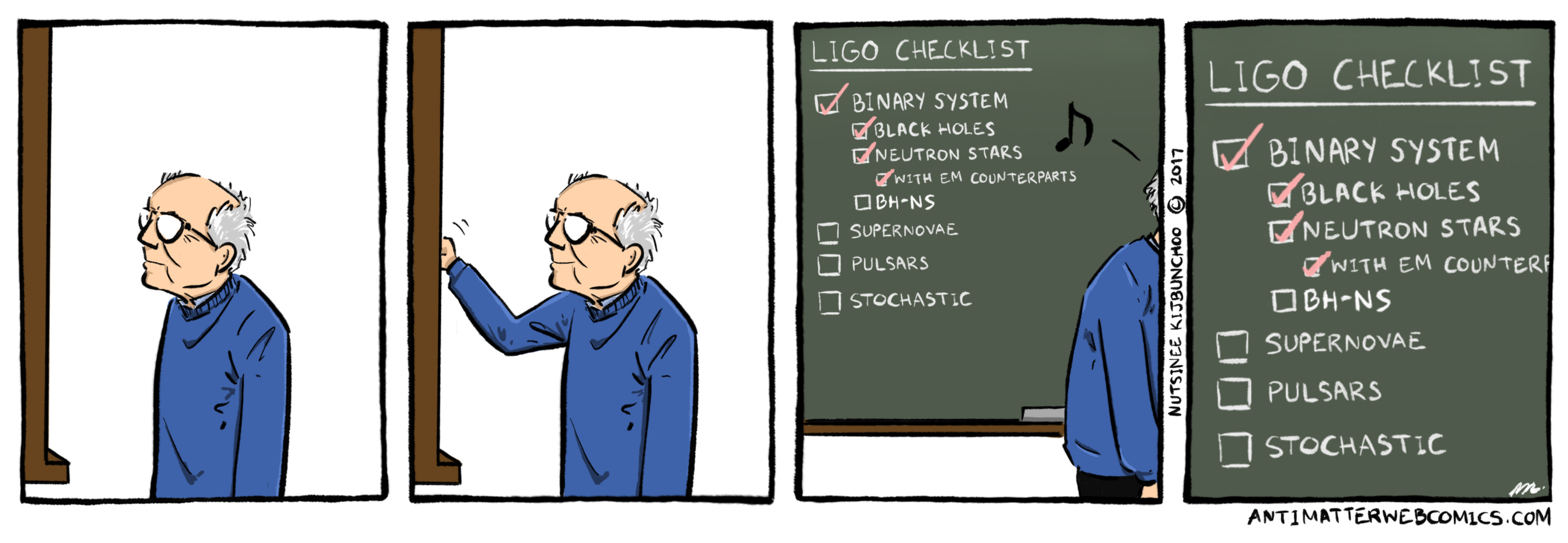

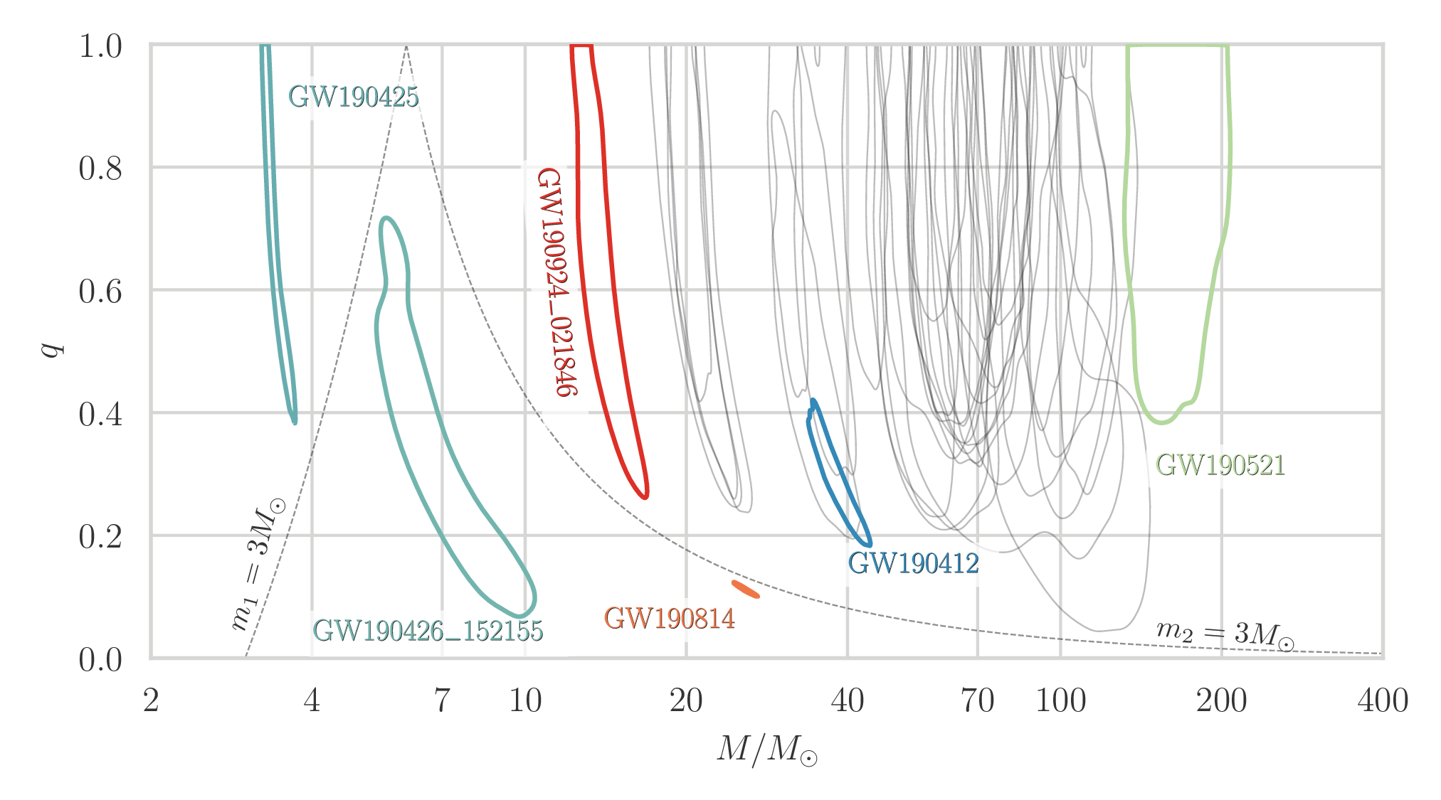


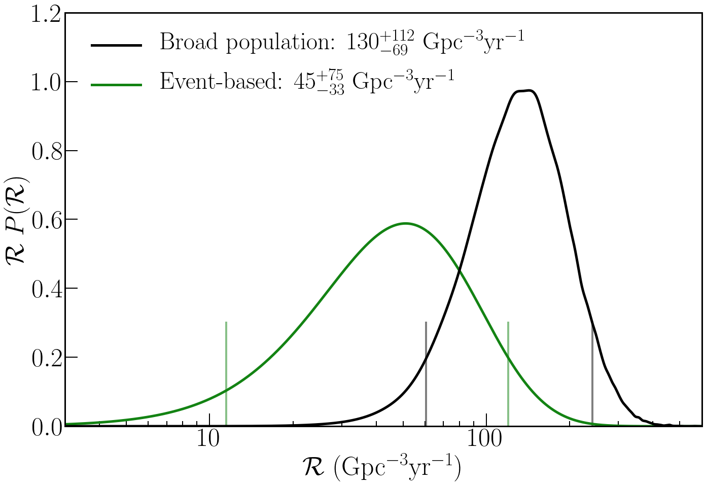


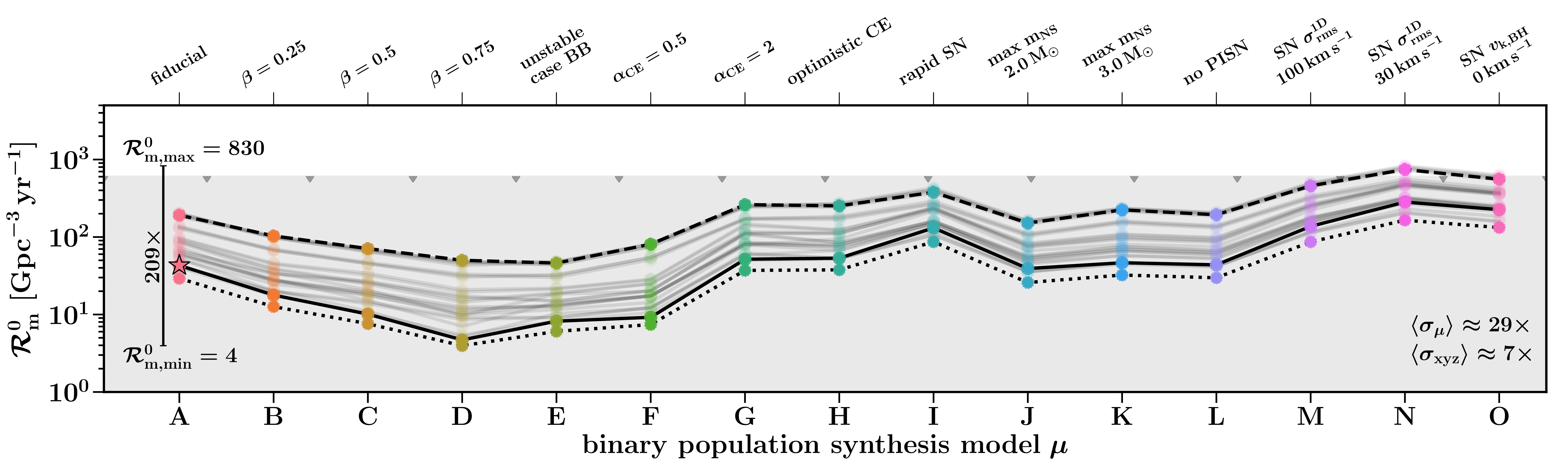


 (where our Sun has a mass of
  and
and  black hole. These massive (or
  black holes). In any case, whatever mechanism created these black holes needs to work quickly, as we know from
 . Credit:
  and
and  . Massive black holes should grow from these smaller black holes. However, we have never found one, they are the
  the merger remnant is without doubt an intermediate-mass black hole.
 and
and  . The large black hole masses extremely difficult to explain.
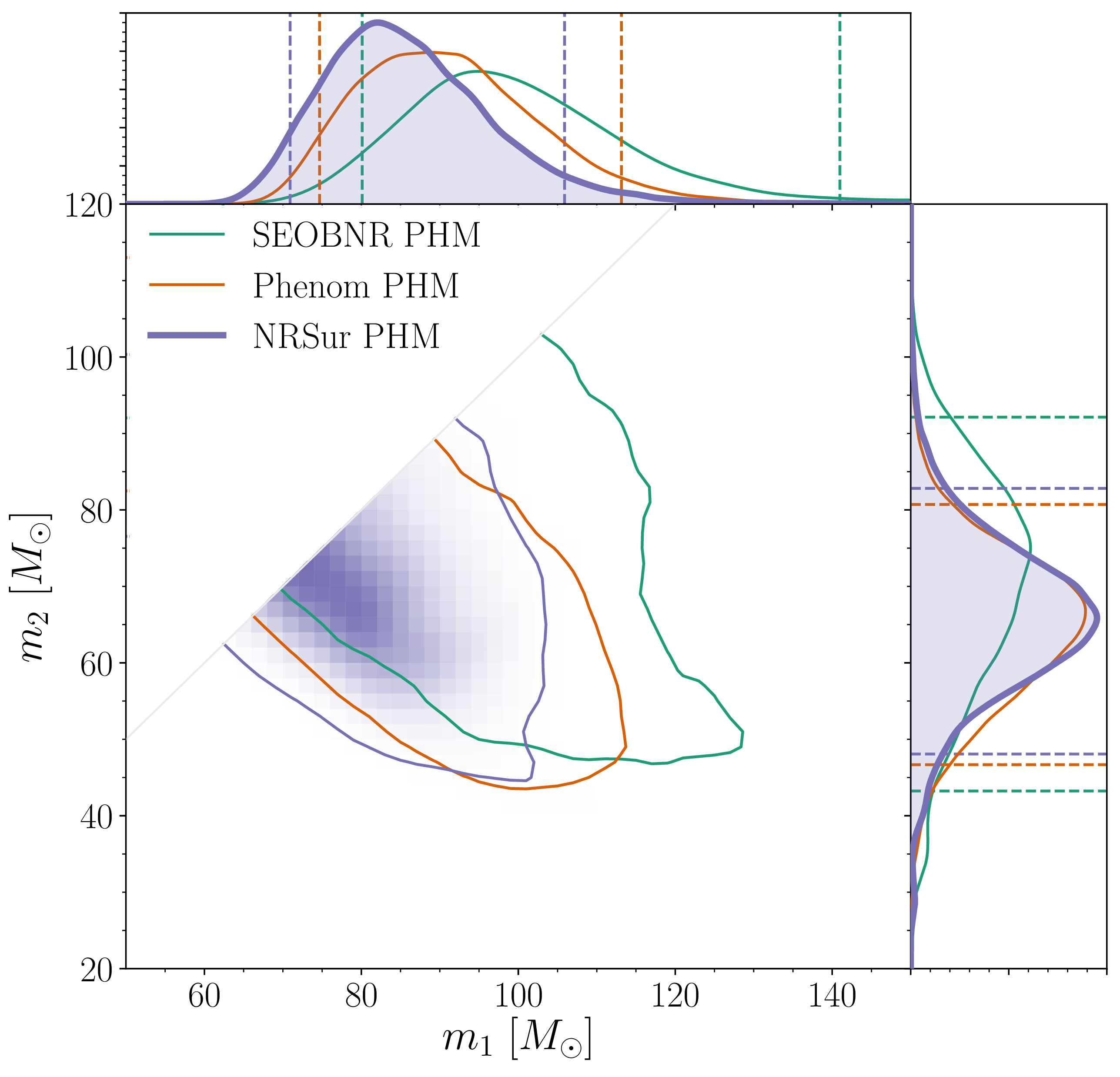
 . We show results several different waveform models and use the
  , just slightly less than the temperature of the mozerlla on that first bite of pizza, even though you should know better by now), the photons of light (gamma-rays) bouncing around inside the core become energetic enough to produce pairs of electrons and positrons [
 . If the core is between
  , the star will blast off its outer layers, possibly repeating the
  , the explosion completely destroys the star, leaving nothing behind. These stars never collapse down to a black hole, and this leaves a
  and
and  .
.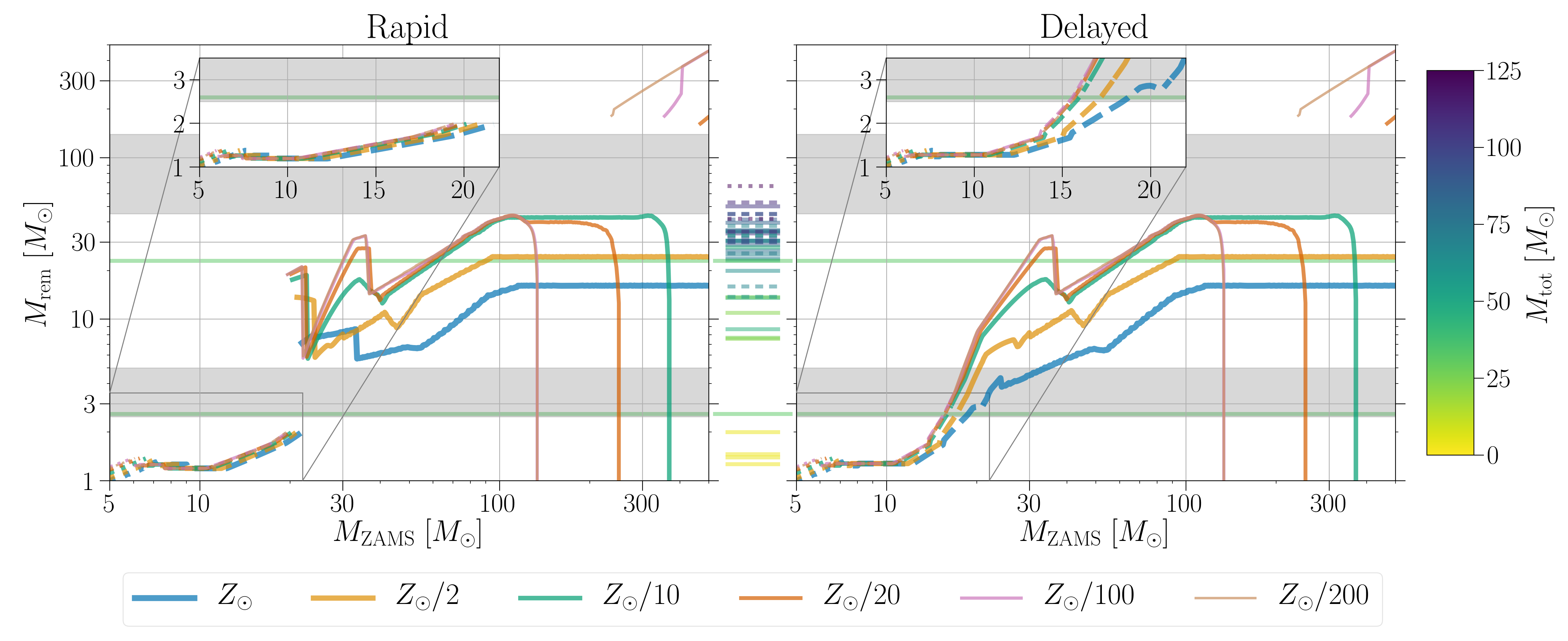
 for different initial (zero age main sequence) stellar masses
  . This is just for single stars, and ignores all the complicated things that can happen in binaries. The different coloured lines indicate different metallicities
  (higher metallicity stars lose more mass through stellar winds). The two panels are for two different supernova models. The grey bars indicate potential mass gaps: the lower core collapse mass gap (only predicted by the Rapid model) and the upper pair-instability mass gap. The tick marks in the middle are various claimed gravitational-wave source, colour-coded by the total mass of the binary
  . Figure 1 of
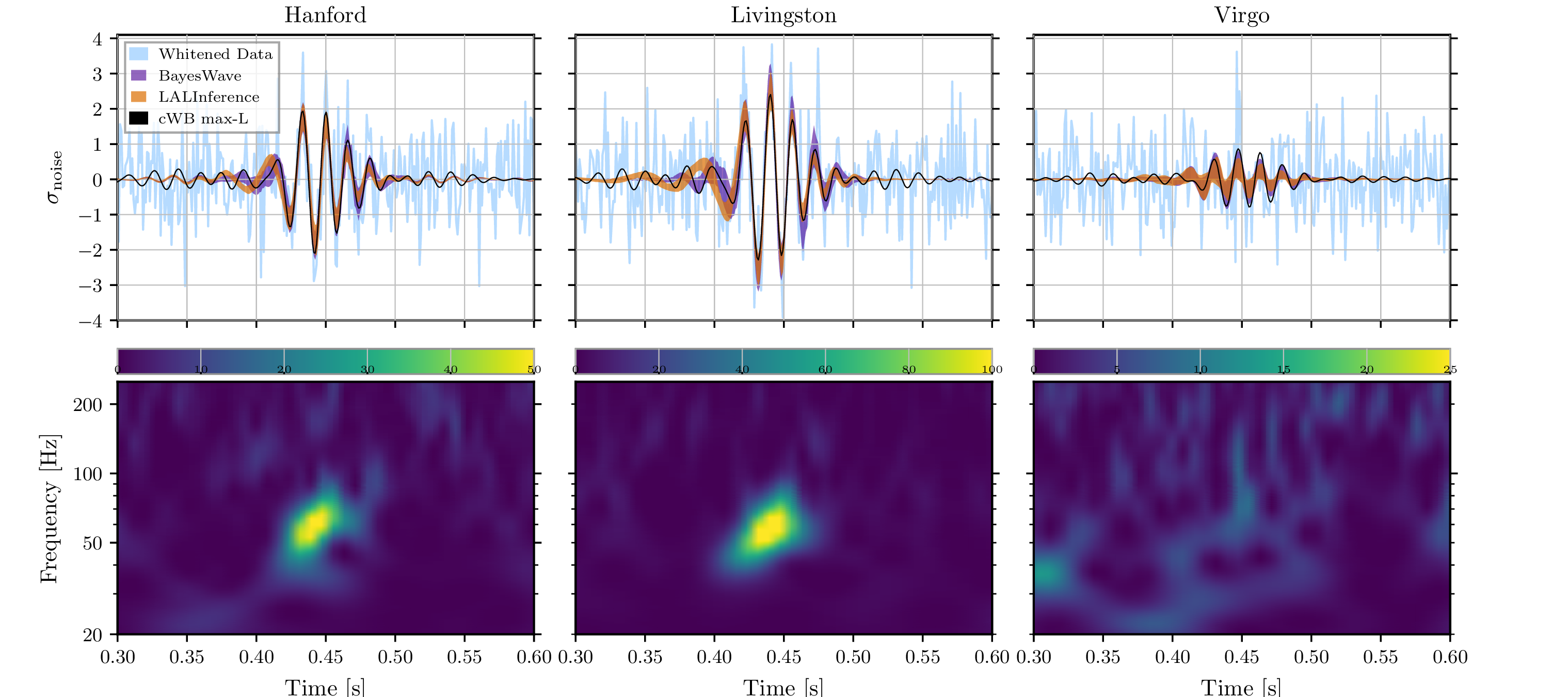
 in favour of the binary signals, so it’s probably not cosmic strings. Finally, you’ve perhaps noticed that I’ve been writing quasicircular [
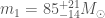 and
and 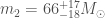 , and that the merger remnant is
 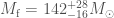 . The plot below shows the final mass as well as the spin, which is
  . For the black holes formed from the mergers of near equal mass binaries, you’d expect the final spin to be around
  .
.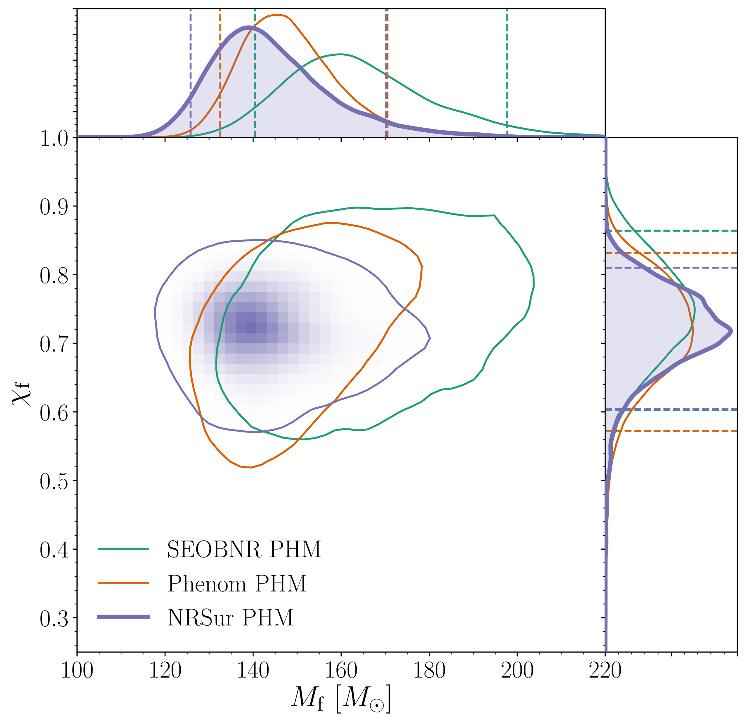
 and spin
  for the final black hole. We show results several different waveform models and use the numerical relativity surrogate (NRSur PHM) as our best results. The two-dimensional shows the 90% probability contour. The dotted lines in one-dimensional plots the symmetric 90% credible interval. The mass is safely above the conventional lower limit to be considered an intermediate-mass black hole. Figure 3 of the
  . Looking at the ringdown, we get lovely consistent results trying ringdown models at different start times and including different higher order multipole moments, and all agree with the analysis of the entire signal using the quasicircular templates.
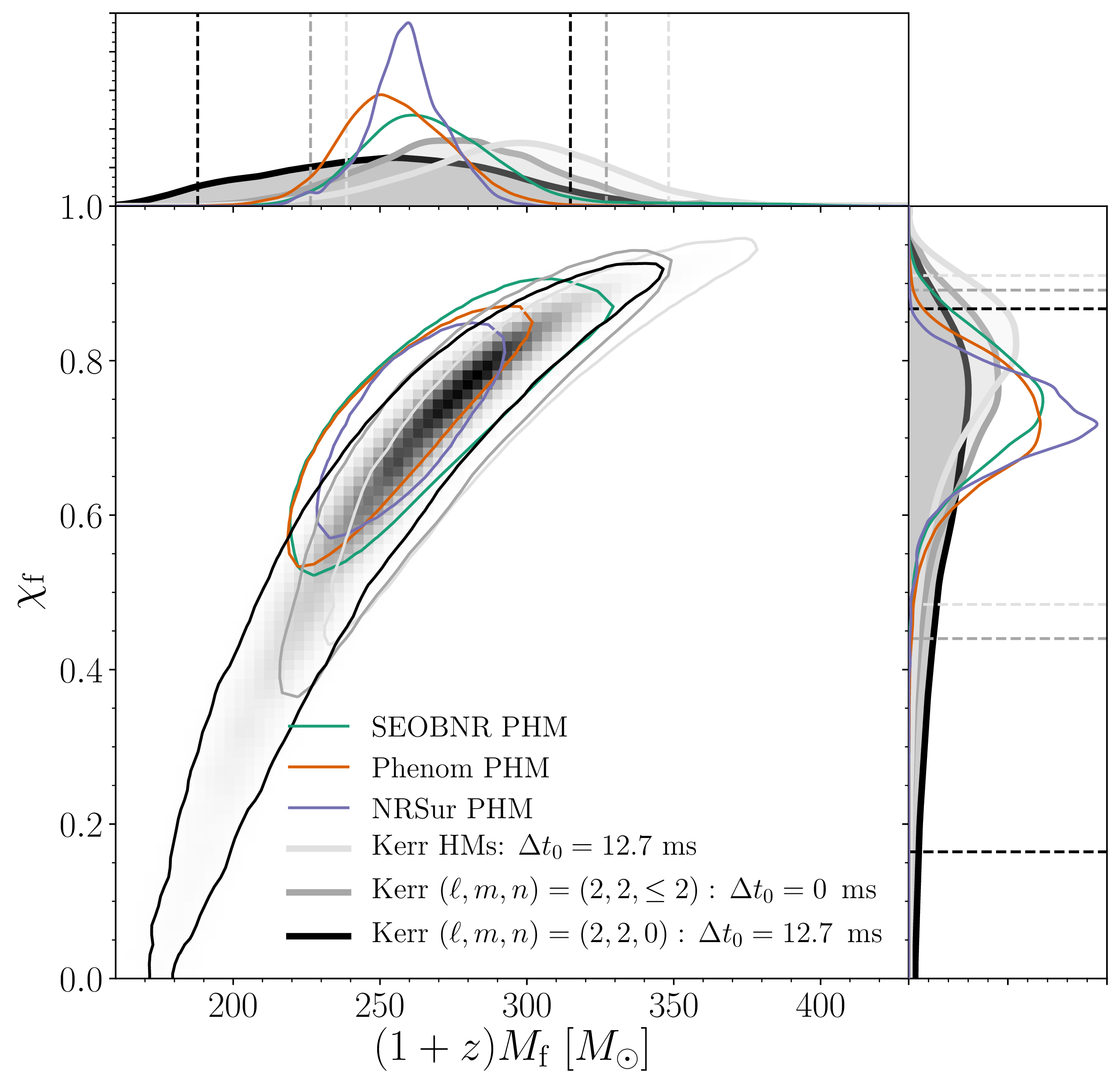
 , which goes from
  for both the spins being maximal and antialigned with the orbital angular momentum to
  for both spins being maximal and aligned with the orbital angular momentum. We find that
  , consistent with no spin, spins antialigned with each other or in the orbital plane. The result is strongly influenced by the assumed prior, we’ve not learnt much from the signal.
 , which goes from
  for no in-plane spin, to
  , but there’s support across the entire range.
 . This makes the source a good contender for the most distant gravitational wave source ever found [
 . This would be OK if sources were uniformly distributed in a non-evolving Universe, but sadly we don’t live in such a thing, and we have to take into account the expansion of the Universe, and the evolution of the galaxies and stars within it. We’ll come back to look at this when we present our catalogue of detections from the first part of the third observing run.
 , but that is extremely speculative (I’d love it if it were true). Sticking to known physics, at face value, it is hard to explain the mass of the primary black hole from our understanding of how stars evolve.
 . Predicted rates for the various formation mechanisms discussed above can be rather uncertain (kind of like how the exact value of a small bag full of
  , what if we tried
  , more like you would expect for a nuclear star cluster? We shouldn’t really be doing this, as our model is calibrated against globular cluster simulations, and nuclear star clusters have different dynamics, but we can use our results as illustrative. In this case, we find odds of about 1000:1 in favour of hierarchical mergers. This suggests that this option may be a promising one to follow, but we must moderate our results remembering that only a fraction of binaries would form in these dense environments.
 in context, if you put
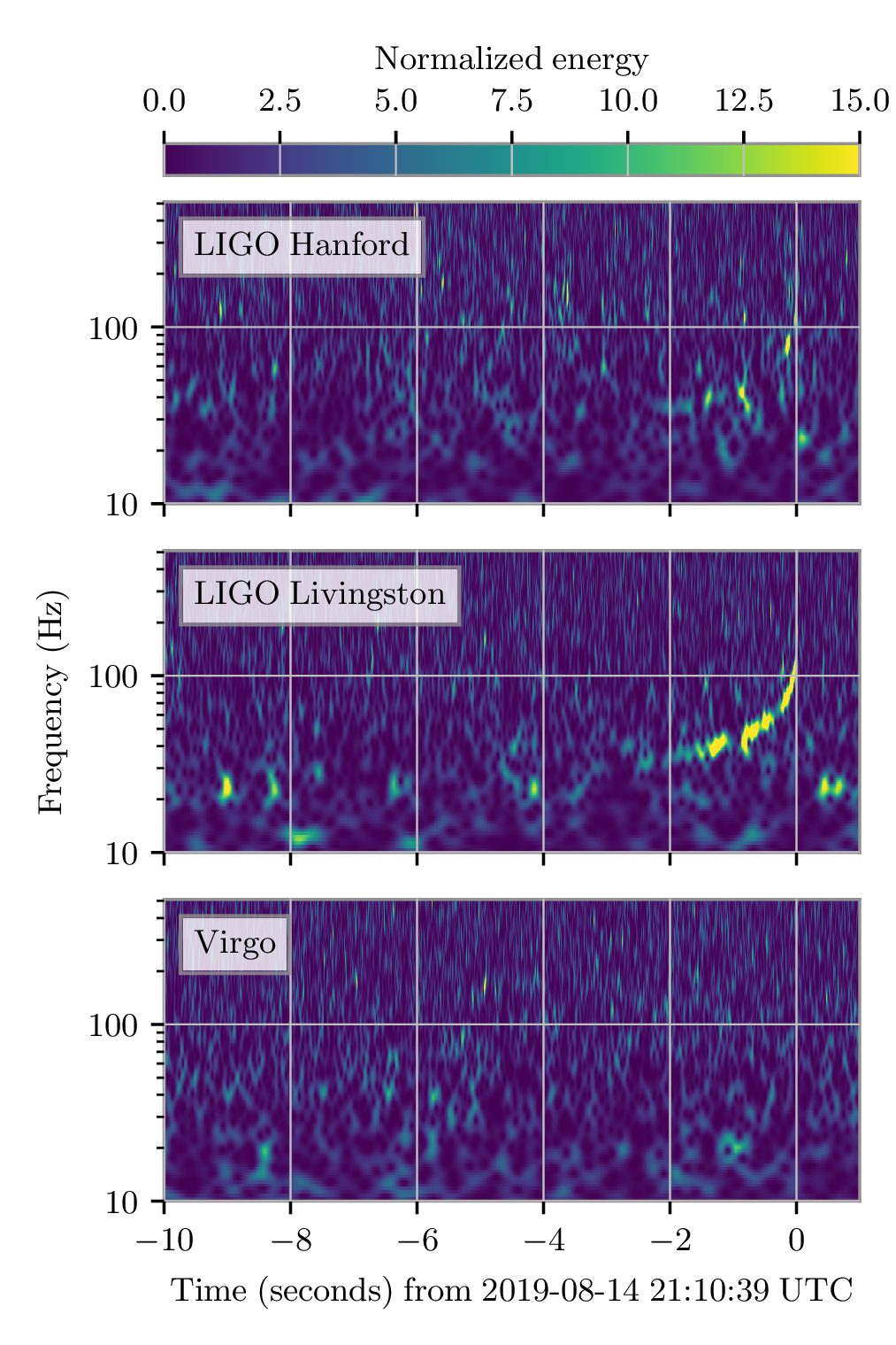

 . All contours are for 90% probabilities. Figure 2 of the
  solar masses (quoting the 90% range for parameters), and the other
  solar masses. This is remarkable for two reasons: first, the lower mass object is right in the range where we might hit the maximum mass of a neutron star, and second, this is the most asymmetric masses from any of our gravitational wave sources.
 . We show results several different waveform models (which include spin precession and higher order multiple moments). The two-dimensional shows the 90% probability contour. The one-dimensional plot shows individual masses; the dotted lines mark 90% bounds away from equal mass. Estimates for the maximum neutron star mass are shown for comparison with the mass of the lighter component
  M&Ms (plain; for peanut butter it would be different, and of course, more delicious) into the volume of just
  M&Ms (ignoring the fact that you can’t perfectly pack them)! Neutron stars are about
  times more dense than M&Ms. As you make neutron stars heavier, their gravity gets stronger until at some point the strange stuff™ they are made of can’t take
  and the tidal deformability
  .
.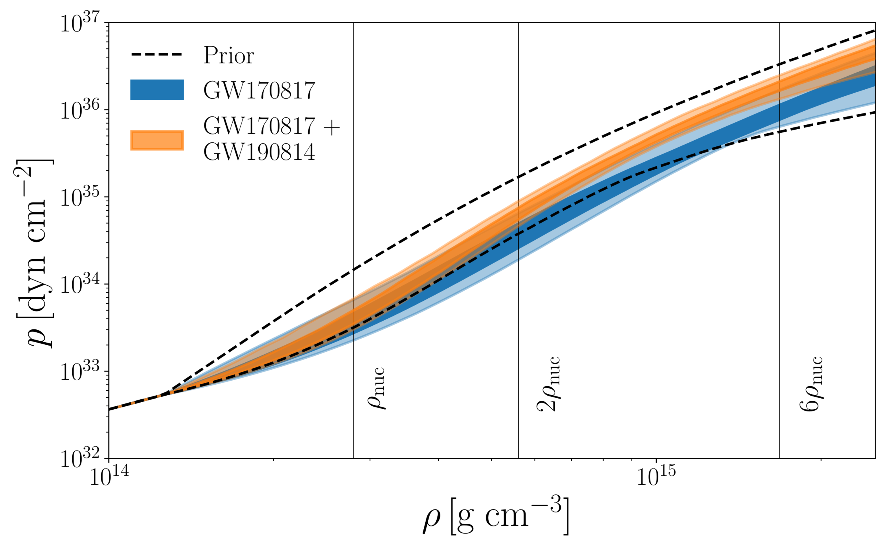
 . The mass ratio changes a few things about the gravitational wave signal. When you have unequal masses, it is possible to observe
  . We again spot the next harmonic in GW190814, this time it is even more clear. Modelling gravitational waves from systems with mass ratios of
  is tricky, it is important to include the higher order multipole moments in order to get good estimates of the source parameters.
 . This is our best ever measurement of black hole spin!
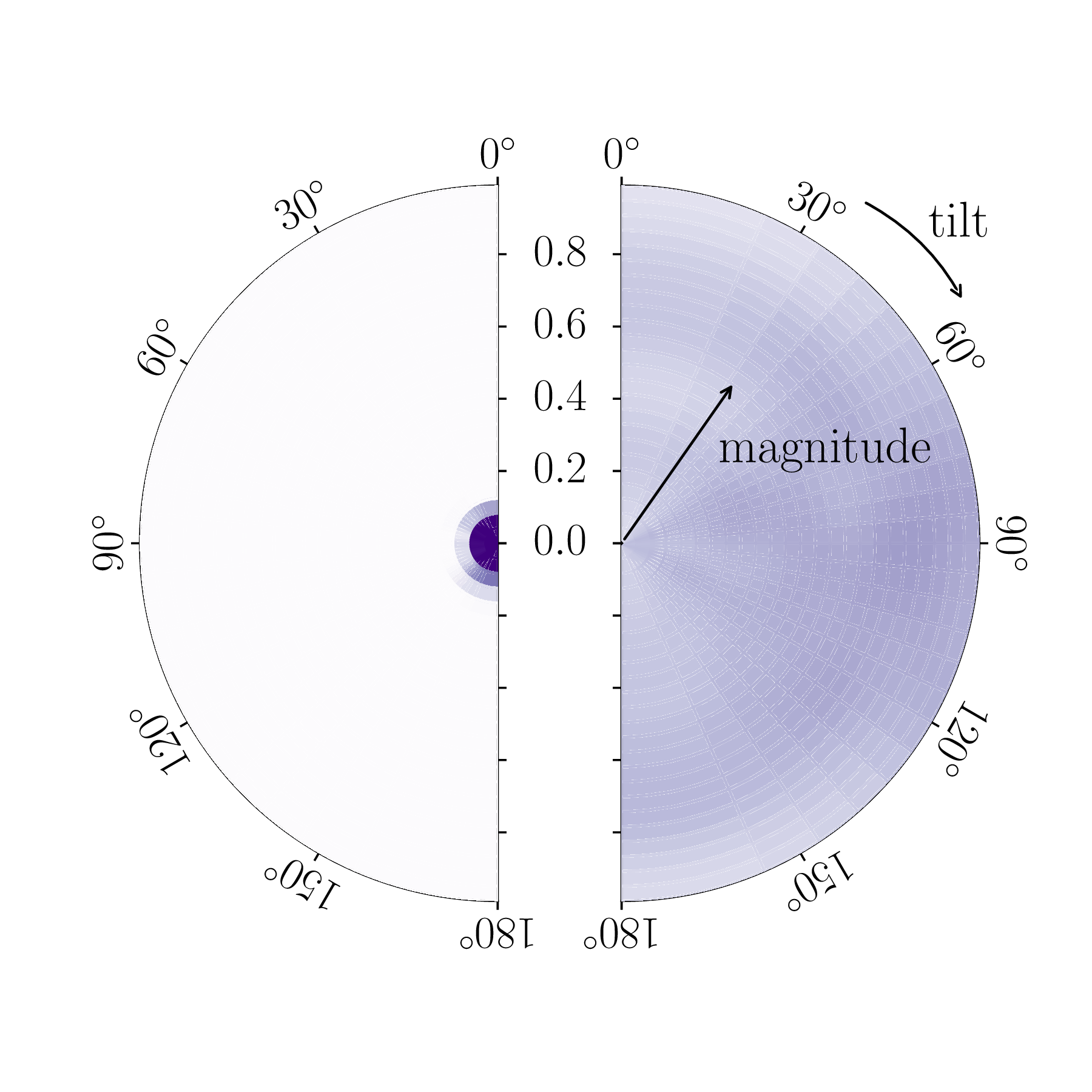
 . Harder to measure is the spin in the orbital plane. This controls the amount of spin precession (wobbling in the spin orientation as the orbital angular momentum is not aligned with the total angular momentum), and is characterised by the effective precession spin parameter. For GW190814, we find
  , which is our tightest measurement. It might seem odd that we get our best measurement of in-plane spin in the case when there is no precession. However, this is because if there were precession, we would clearly measure it. Since there is no support for precession in the data, we know that it isn’t there, and hence that the amount of in-plane spin is small.
 . From GW190814 alone, we get
  (quoting numbers with our usual median and symmetric 90% interval convention; if you like mode and narrowest 68% region, it’s
  ). If we combine with results for GW170817, we get
  (or
(or  ) [
) [ . If you think you know how GW190814 formed, you’ll need to make sure to get a compatible rate estimate.
 is the orbital separation,
  is the orbital inclination,
  is the time since the stars started their life on the main sequence. The letters on the right indicate the evolution phase: ZAMS is zero-age main sequence, MS is main sequence (burning hydrogen), CHeB is core helium burning (once the hydrogen has been used up), and BH and NS mean black hole and neutron star. At low metallicities
  . The luminosity distance is a measure which incorporates the effects of the signal travelling through an expanding Universe, so it’s not quite the same as the actual distance between us and the source. Given the uncertainties on the luminosity distance, it would have taken the signal somewhere between 600 million and 850 million years to reach us. It therefore set out during the
  calories. That seems like a lot of energy, but it’s less than
  of the energy emitted as gravitational waves for GW190814.
 (mode and narrowest 68% region) using GW190814. Adding in GW170814 they get
  as a gravitational-wave-only measurement, and including GW170817 and its electromagnetic counterpart gives
  .
.
 times the mass of our Sun (quoting the 90% range for parameters), and the other
  times the mass of our Sun. Neither of these masses is too surprising on their own. We know black holes come in these sizes. What is new is the ratio of the masses
 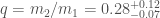 [
[
 for the two components in the binary and the effective inspiral spin
  ,
, and
and  are the spins of the two black holes [
 and
and  are the tilts angles measuring the alignment of the spins with the orbital angular momentum. The spins change orientations during the inspiral if they are not perfectly aligned with the orbital angular momentum, which is referred to as precession, but
 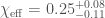 .
. .
. . This is the best measurement of
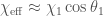 ), and similarly
  ). Combining all this information, we can actually get a good measurement of the spin of the bigger black hole. We infer that
  . This is the first time we’ve really been able to measure an individual spin!
 , where we use
  as the angles on the sphere, and
  specify the harmonic. The majority of the gravitational radiation emitted from a binary is from the
  harmonic, so we usually start with this. Larger values of
  contribute less and less. For exactly equal mass binaries with non-spinning components, only harmonics with even
  are expected to contribute a significant amount. In previous detection, we’ve not had to worry too much about the harmonics with
  , which we refer to as higher order multipole moments, as they contributed little to the signal. GW190412’s unequal masses mean that they are important here.
 , where
  is the orbital frequency. Most of the signal is emitted at twice the orbital frequency, but the emission from the higher order multipoles is at higher frequencies. If the
  multipole was a music A, then the
  multipole would correspond to an E, and if the
  showing the significance of the
  mode. This shows that the harmonic structure of gravitational waves is as expected [
 , corresponding to a travel time for the signal of around 2 billion years) using templates calculated using only the
  harmonic.
 and estimated the value of
  . A result of
  would mean that all mass ratios were equally common, while larger values would mean that binaries liked more equal mass binaries. Our analysis preferred larger values of
 to
to  , but we see that the mass ratio is still clearly unequal.
 of the time. Therefore, GW190412 is exceptional, but not completely inconsistent with our previous observations. If we repeat the calculation using the population inferred folding in GW190412, we (unsurprisingly) find it is much less unusual, with such systems being found in a set of eleven observations
  of the time. In conclusion, GW190412 is not vanilla, but is possibly raspberry ripple or Neapolitan: there’s still a trace of vanilla in there to connect it to the more usual binaries
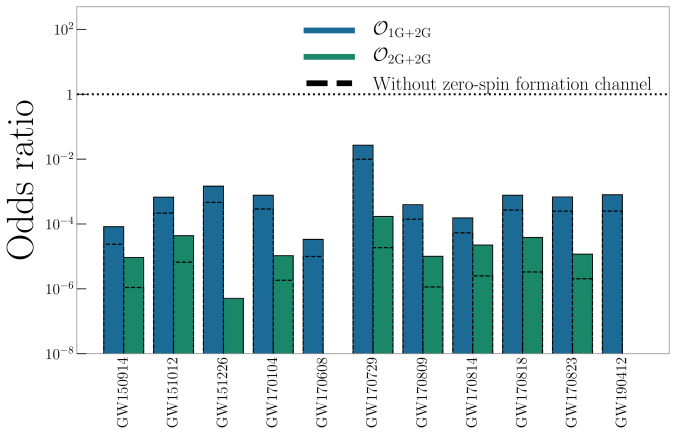
 , meaning that the mass ratio spans the entirely sensible range of
  , and those heretics who define
  , meaning that it cover the ridiculous range of
  . Within LIGO and Virgo, we have now settled on the correct convention. Many lives may have been lost, but I’m sure you’ll agree that it is a sacrifice worth making in the cause of consistent notation.
 (the Greek letter chi) and
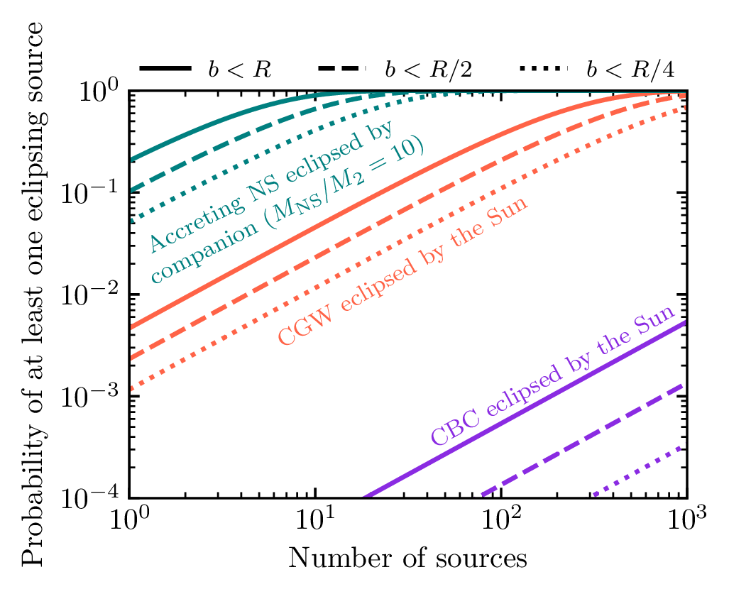
 of the centre of the star. Figure 1 of
 . This is may just contain noise,
  , or it may also contain a signal,
  .
. . On average we expect the noise at a given frequency to be zero, but with it fluctuating up and down with a variance given by the power spectral density. We typically approximate the noise as Gaussian, such that
 ,
, to represent a normal distribution with mean
  and standard deviation
  . The approximations of stationary and Gaussian noise are good most of the time. The noise does vary over time, but is usually effectively stationary over the durations we look at for a signal. The noise is also mostly Gaussian except for glitches. These are taken into account when we search for signals, but we’ll ignore them for now. The statistical description of the noise in terms of the power spectral density allows us to understand our data, but this understanding comes as a function of frequency: we must transform of time domain data to frequency domain data.
 we can use a Fourier transform. Fourier transforms are a way of converting a function of one variable into a function of a reciprocal variable—in the case of time you convert to frequency. Fourier transforms encode all the information of the original function, so it is possible to convert back and forth as you like. Really, a Fourier transform is just another way of looking at the same function.
 .
. where
where  is some
  .
. is a
is a 
![d_\mathrm{w}(f) \propto d(f)/[S_n(f)]^{1/2}](https://s0.wp.com/latex.php?latex=d_%5Cmathrm%7Bw%7D%28f%29+%5Cpropto+d%28f%29%2F%5BS_n%28f%29%5D%5E%7B1%2F2%7D&bg=ffffff&fg=444444&s=0&c=20201002) . This is known as
. This is known as  , as the properties of the noise mean that
  . Combining the likelihood for each individual frequency gives the overall likelihood
![\displaystyle p(d|h) \propto \exp\left[-\int_{-\infty}^{\infty} \frac{|d(f) - h(f)|^2}{S_n(f)} \mathrm{d}f \right]](https://s0.wp.com/latex.php?latex=%5Cdisplaystyle+p%28d%7Ch%29+%5Cpropto+%5Cexp%5Cleft%5B-%5Cint_%7B-%5Cinfty%7D%5E%7B%5Cinfty%7D+%5Cfrac%7B%7Cd%28f%29+-+h%28f%29%7C%5E2%7D%7BS_n%28f%29%7D+%5Cmathrm%7Bd%7Df+%5Cright%5D&bg=ffffff&fg=444444&s=0&c=20201002) .
.
 ,
, is the relative difference in the length of the two arms, and
  is the usually arm length. Since we love jargon in LIGO & Virgo, we’ll often refer to the strain as HOFT (as you would read
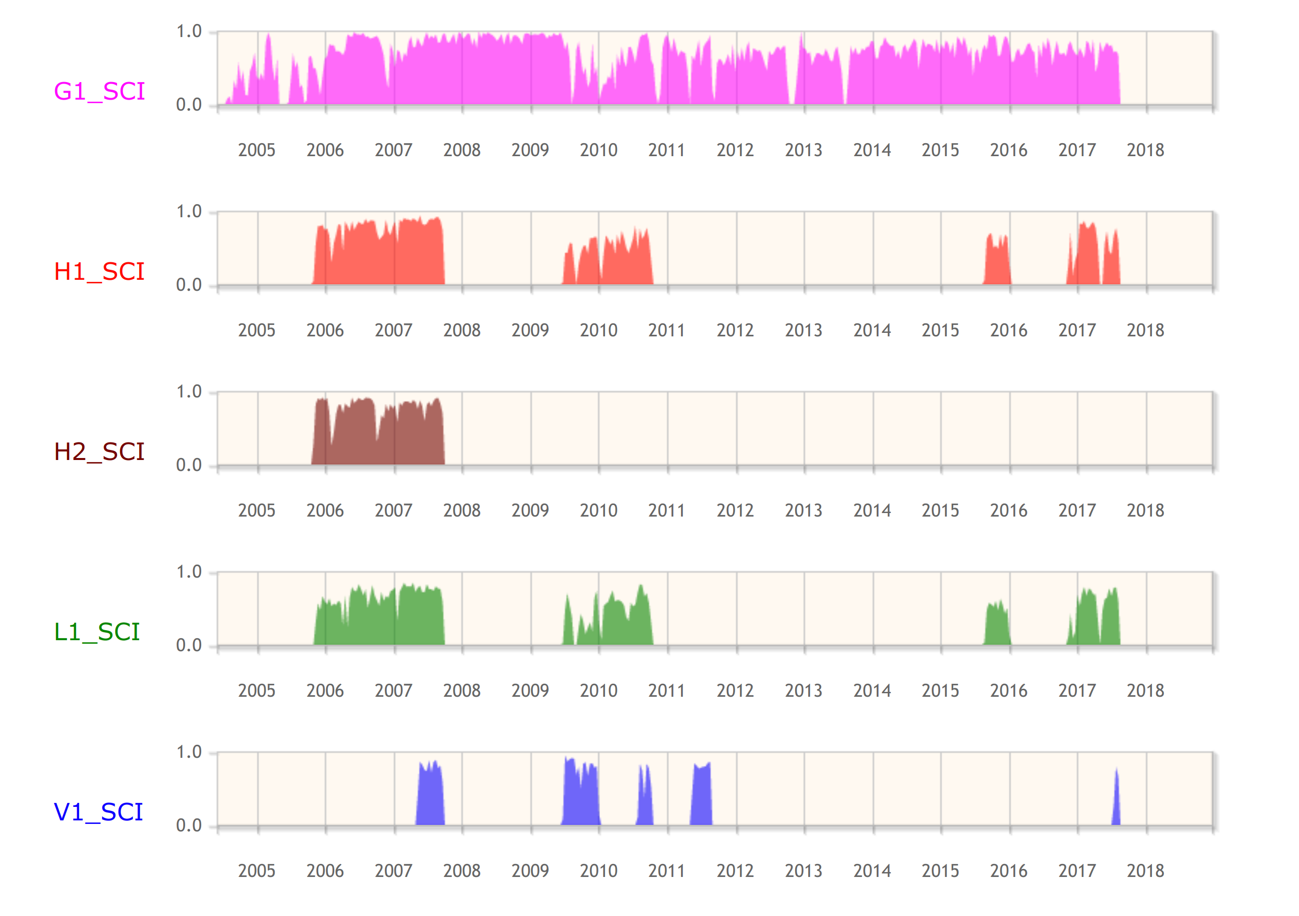


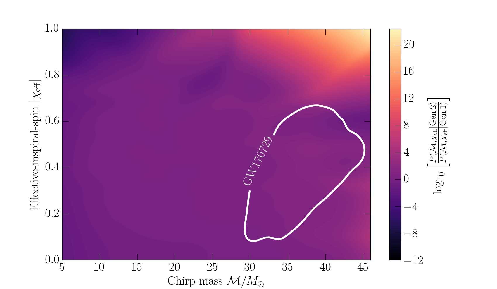
 .
. ,
, .
.

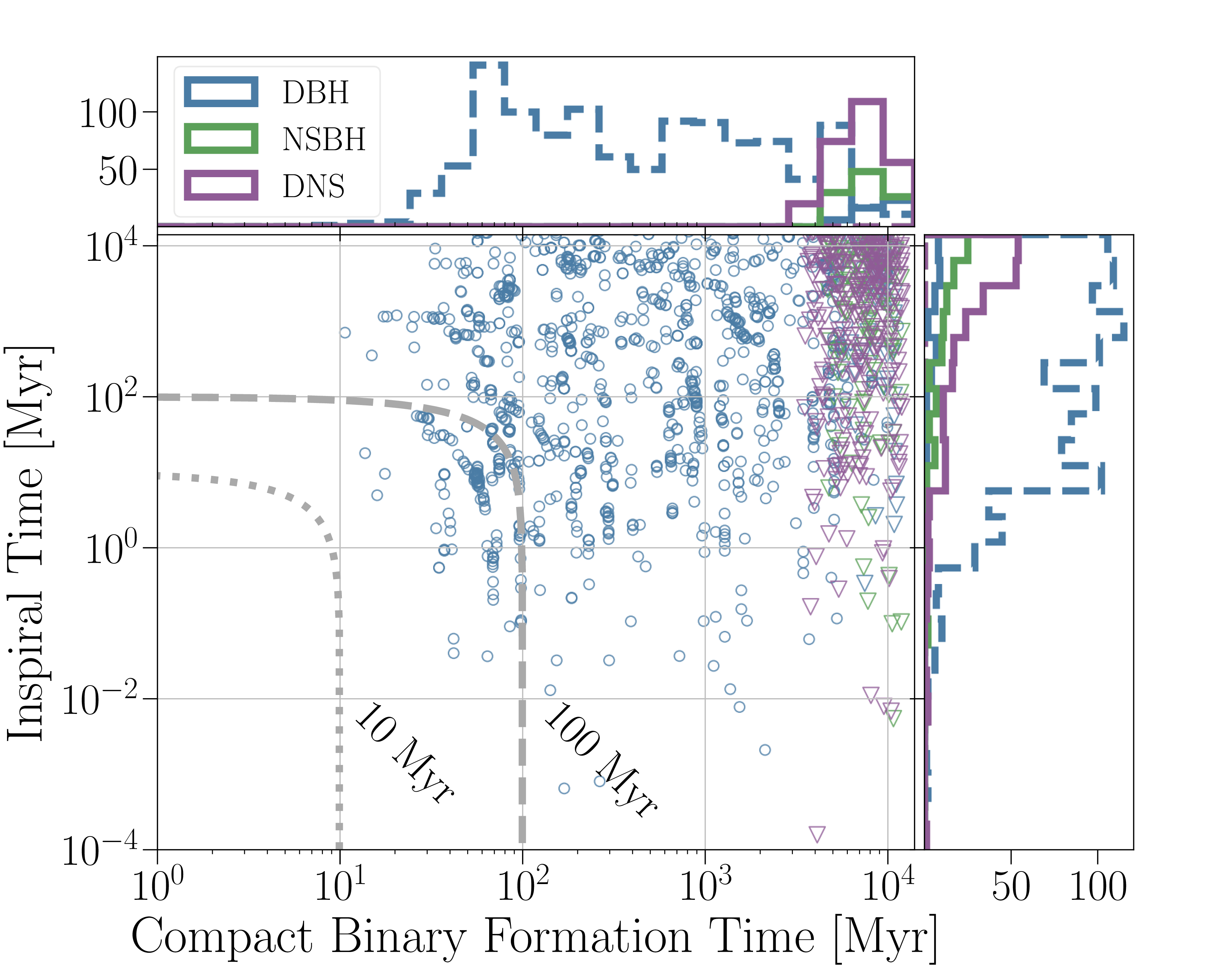

 vs inspiral time
  , and orbital separation
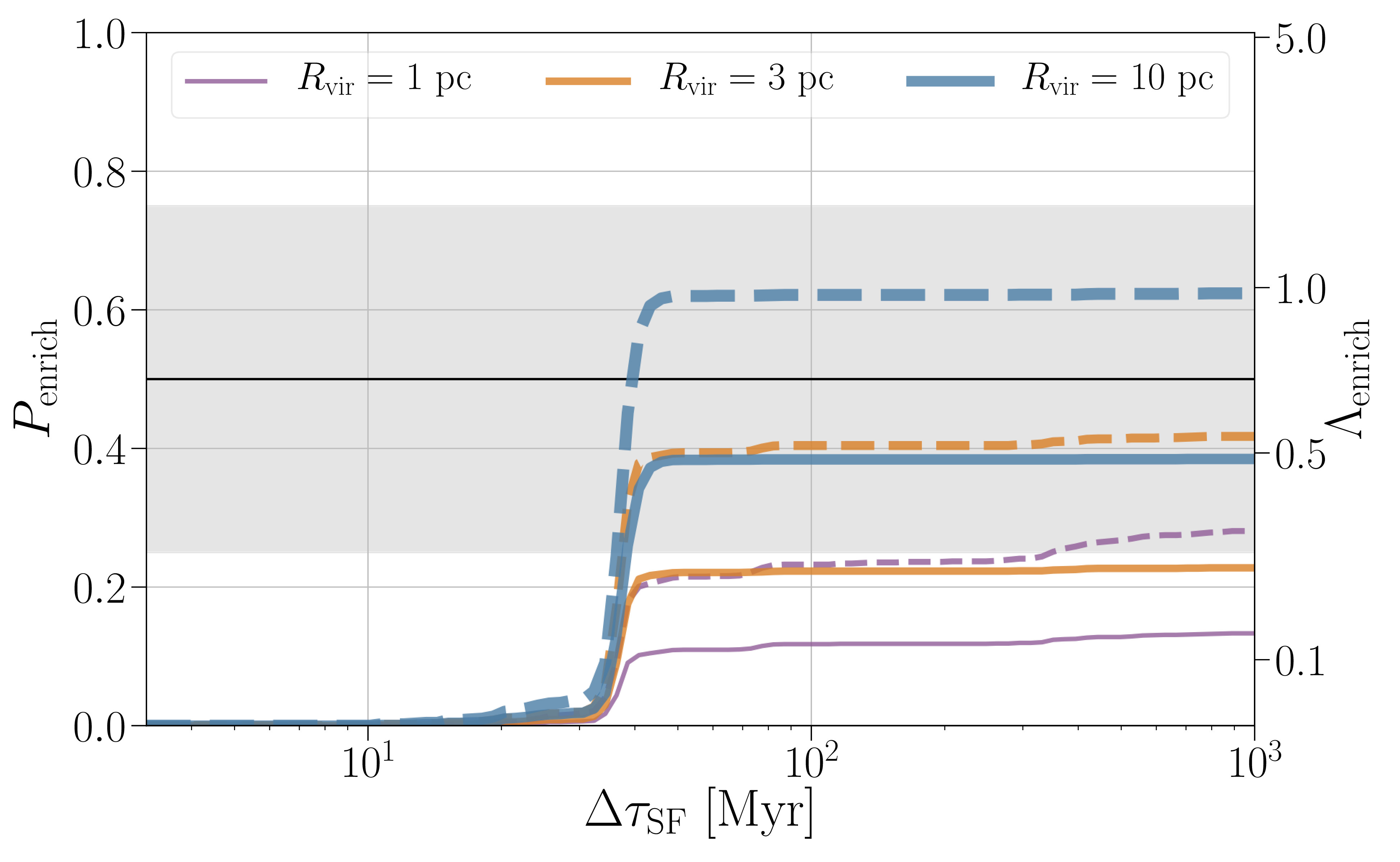
 and number of enriching binary neutron star mergers per cluster
  as a function of the timescale of star formation
  . Dashed lines are used of a cluster of a million solar masses and solid lines are used for a cluster of half this mass. Results are shown for Model D. The build up happens around the same time in different models. Figure 5 in
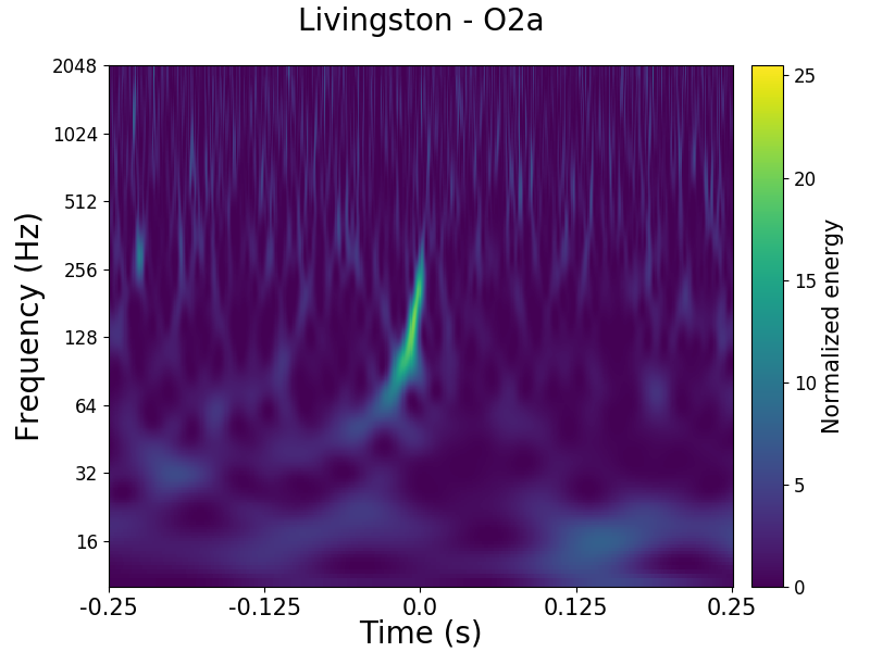


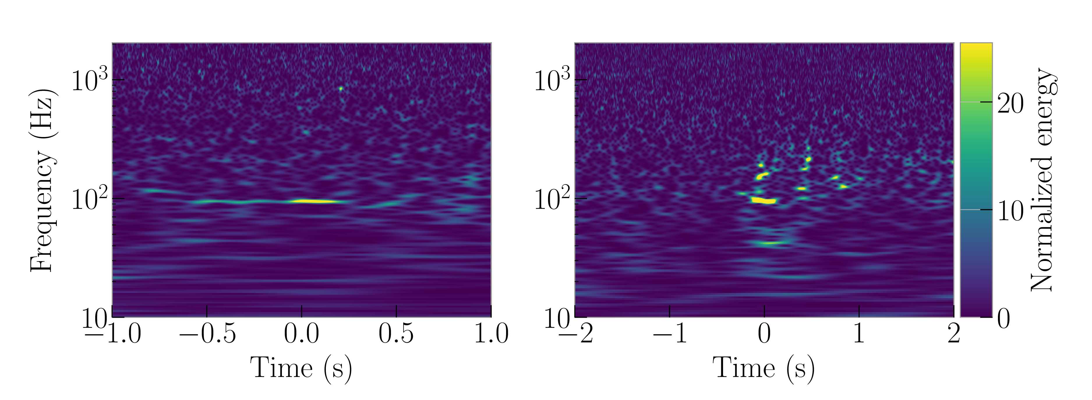
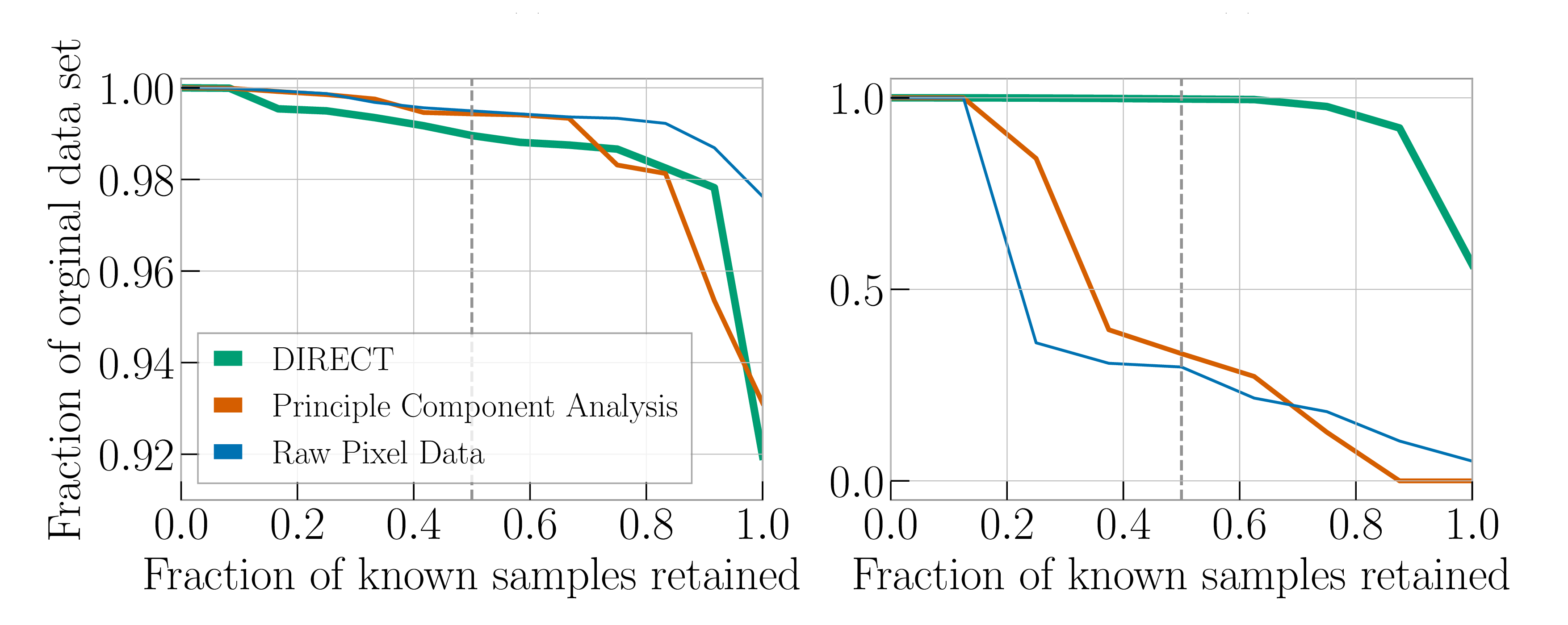
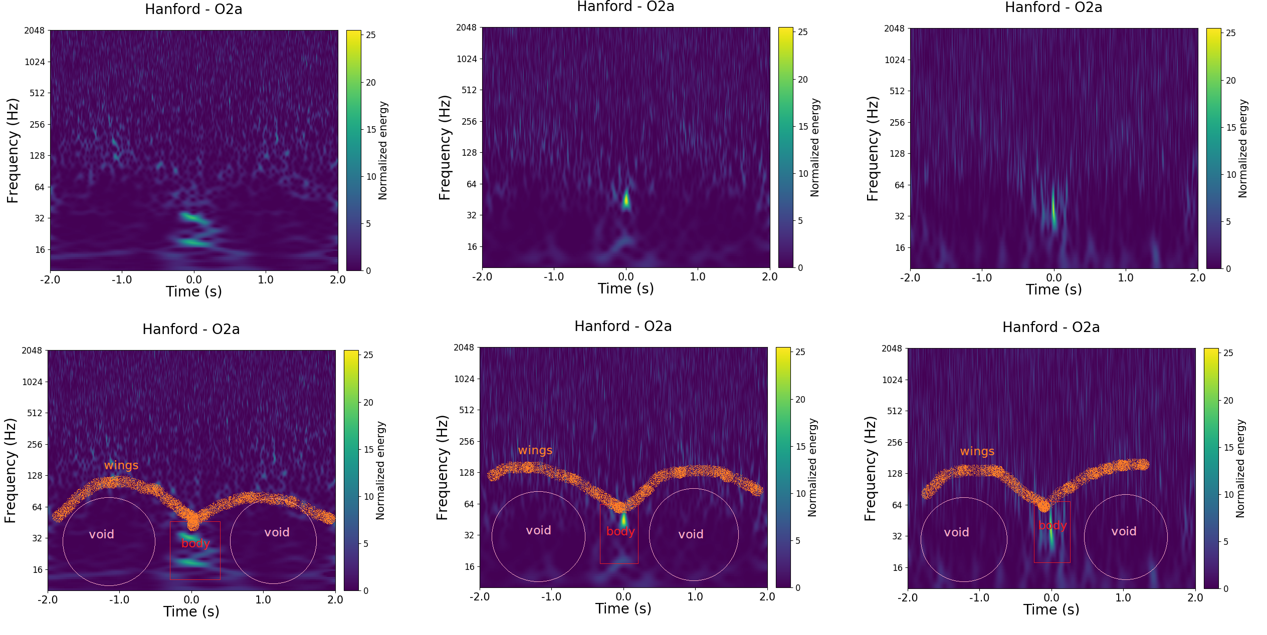


 solar masses (quoting the 90% range for parameters). This is larger than GW170817’s
  solar masses: we have a heavier binary.
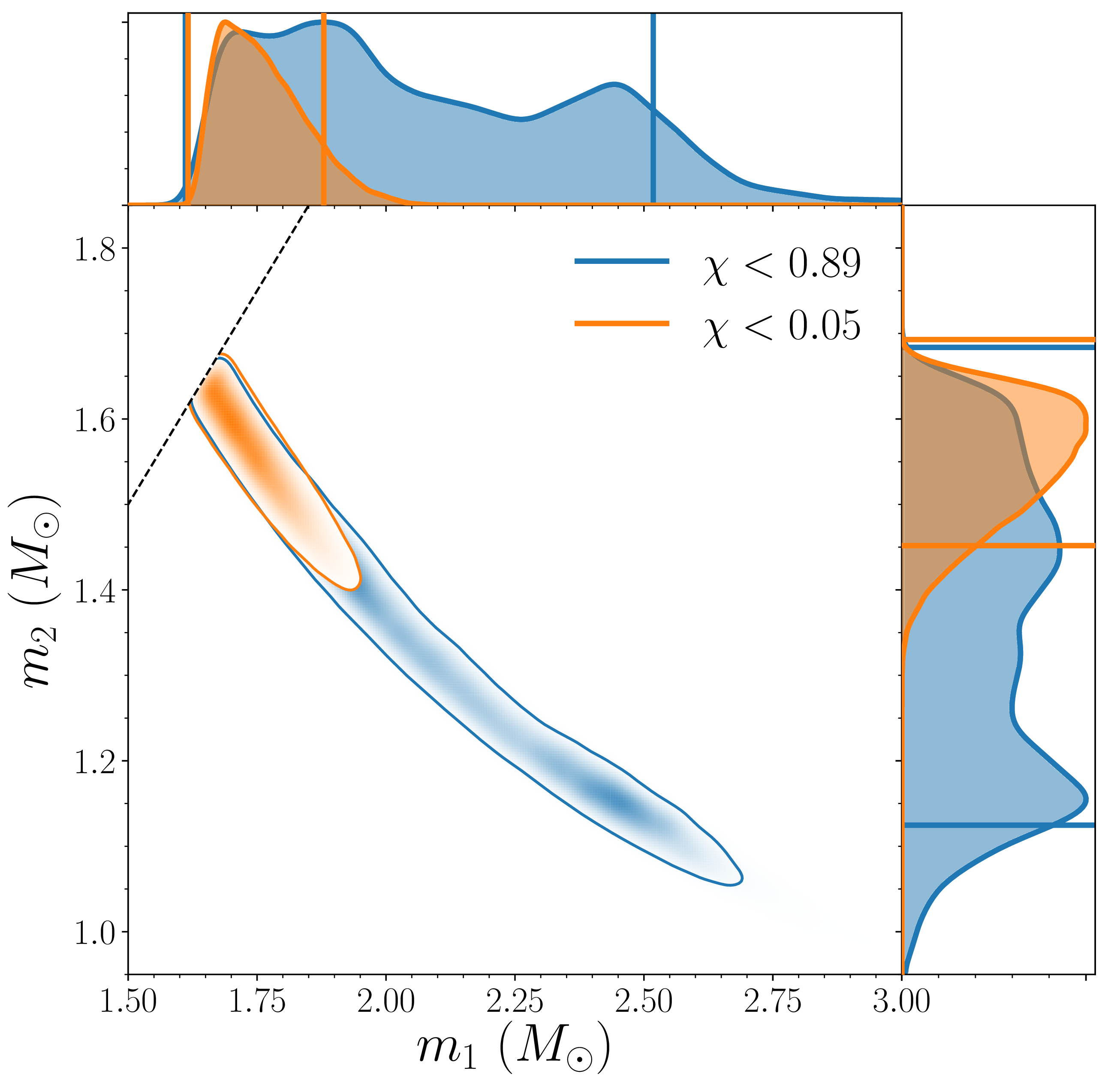
 –
– solar masses with the low-spin assumption, and
  –
– solar masses with the high-spin assumption; the lighter component has a mass
  –
– solar masses with the low-spin assumption, and
  –
– solar masses with the high-spin. These are the range of masses expected for neutron stars.
 . That means the signal was travelling across the Universe for about half a billion years. This is as many times bigger than diameter of Earth’s orbit about the Sun, as the diameter of the orbit is than the height of a LEGO brick. Space is big.
 –
–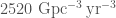 . Now, adding in the first 50 days of O3, we estimate the rate to be
  –
– , so roughly the same (which is nice) [
 , and the GW190425-like rate is lower at
  –
– . Combining the two (Assuming that binary neutron stars are all one class or the other), gives an overall rate of
  –
– , which is not too different than assuming the uniform distribution of masses.
