Accuracy of inference on the physics of binary evolution from gravitational-wave observations

June 11, 2018July 9, 2019 / CPLB / Leave a comment

Gravitational-wave astronomy lets us observing binary black holes. These systems, being made up of two black holes, are pretty difficult to study by any other means. It has long been argued that with this new information we can unravel the mysteries of stellar evolution. Just as a palaeontologist can discover how long-dead animals lived from their bones, we can discover how massive stars lived by studying their black hole remnants. In this paper, we quantify how much we can really learn from this black hole palaeontology—after 1000 detections, we should pin down some of the most uncertain parameters in binary evolution to a few percent precision.

Life as a binary

There are many proposed ways of making a binary black hole. The current leading contender is isolated binary evolution: start with a binary star system (most stars are in binaries or higher multiples, our lonesome Sun is a little unusual), and let the stars evolve together. Only a fraction will end with black holes close enough to merge within the age of the Universe, but these would be the sources of the signals we see with LIGO and Virgo. We consider this isolated binary scenario in this work [bonus note].

Now, you might think that with stars being so fundamentally important to astronomy, and with binary stars being so common, we’d have the evolution of binaries figured out by now. It turns out it’s actually pretty messy, so there’s lots of work to do. We consider constraining four parameters which describe the bits of binary physics which we are currently most uncertain of:

Black hole natal kicks—the push black holes receive when they are born in supernova explosions. We now the neutron stars get kicks, but we’re less certain for black holes [bonus note].
Common envelope efficiency—one of the most intricate bits of physics about binaries is how mass is transferred between stars. As they start exhausting their nuclear fuel they puff up, so material from the outer envelope of one star may be stripped onto the other. In the most extreme cases, a common envelope may form, where so much mass is piled onto the companion, that both stars live in a single fluffy envelope. Orbiting inside the envelope helps drag the two stars closer together, bringing them closer to merging. The efficiency determines how quickly the envelope becomes unbound, ending this phase.
Mass loss rates during the Wolf–Rayet (not to be confused with Wolf 359) and luminous blue variable phases–stars lose mass through out their lives, but we’re not sure how much. For stars like our Sun, mass loss is low, there is enough to gives us the aurora, but it doesn’t affect the Sun much. For bigger and hotter stars, mass loss can be significant. We consider two evolutionary phases of massive stars where mass loss is high, and currently poorly known. Mass could be lost in clumps, rather than a smooth stream, making it difficult to measure or simulate.

We use parameters describing potential variations in these properties are ingredients to the COMPAS population synthesis code. This rapidly (albeit approximately) evolves a population of stellar binaries to calculate which will produce merging binary black holes.

The question is now which parameters affect our gravitational-wave measurements, and how accurately we can measure those which do?

Merger rate with redshift and chirp mass

Binary black hole merger rate at three different redshifts $z$ as calculated by COMPAS. We show the rate in 30 different chirp mass bins for our default population parameters. The caption gives the total rate for all masses. Figure 2 of Barrett et al. (2018)

Gravitational-wave observations

For our deductions, we use two pieces of information we will get from LIGO and Virgo observations: the total number of detections, and the distributions of chirp masses. The chirp mass is a combination of the two black hole masses that is often well measured—it is the most important quantity for controlling the inspiral, so it is well measured for low mass binaries which have a long inspiral, but is less well measured for higher mass systems. In reality we’ll have much more information, so these results should be the minimum we can actually do.

We consider the population after 1000 detections. That sounds like a lot, but we should have collected this many detections after just 2 or 3 years observing at design sensitivity. Our default COMPAS model predicts 484 detections per year of observing time! Honestly, I’m a little scared about having this many signals…

For a set of population parameters (black hole natal kick, common envelope efficiency, luminous blue variable mass loss and Wolf–Rayet mass loss), COMPAS predicts the number of detections and the fraction of detections as a function of chirp mass. Using these, we can work out the probability of getting the observed number of detections and fraction of detections within different chirp mass ranges. This is the likelihood function: if a given model is correct we are more likely to get results similar to its predictions than further away, although we expect their to be some scatter.

If you like equations, the from of our likelihood is explained in this bonus note. If you don’t like equations, there’s one lurking in the paragraph below. Just remember, that it can’t see you if you don’t move. It’s OK to skip the equation.

To determine how sensitive we are to each of the population parameters, we see how the likelihood changes as we vary these. The more the likelihood changes, the easier it should be to measure that parameter. We wrap this up in terms of the Fisher information matrix. This is defined as

$\displaystyle F_{ij} = -\left\langle\frac{\partial^2\ln \mathcal{L}(\mathcal{D}|\left\{\lambda\right\})}{\partial \lambda_i \partial\lambda_j}\right\rangle$ ,

where $\mathcal{L}(\mathcal{D}|\left\{\lambda\right\})$ is the likelihood for data $\mathcal{D}$ (the number of observations and their chirp mass distribution in our case), $\left\{\lambda\right\}$ are our parameters (natal kick, etc.), and the angular brackets indicate the average over the population parameters. In statistics terminology, this is the variance of the score, which I think sounds cool. The Fisher information matrix nicely quantifies how much information we can lean about the parameters, including the correlations between them (so we can explore degeneracies). The inverse of the Fisher information matrix gives a lower bound on the covariance matrix (the multidemensional generalisation of the variance in a normal distribution) for the parameters $\left\{\lambda\right\}$ . In the limit of a large number of detections, we can use the Fisher information matrix to estimate the accuracy to which we measure the parameters [bonus note].

We simulated several populations of binary black hole signals, and then calculate measurement uncertainties for our four population uncertainties to see what we could learn from these measurements.

Results

Using just the rate information, we find that we can constrain a combination of the common envelope efficiency and the Wolf–Rayet mass loss rate. Increasing the common envelope efficiency ends the common envelope phase earlier, leaving the binary further apart. Wider binaries take longer to merge, so this reduces the merger rate. Similarly, increasing the Wolf–Rayet mass loss rate leads to wider binaries and smaller black holes, which take longer to merge through gravitational-wave emission. Since the two parameters have similar effects, they are anticorrelated. We can increase one and still get the same number of detections if we decrease the other. There’s a hint of a similar correlation between the common envelope efficiency and the luminous blue variable mass loss rate too, but it’s not quite significant enough for us to be certain it’s there.

Correaltions between population parameters

Fisher information matrix estimates for fractional measurement precision of the four population parameters: the black hole natal kick $\sigma_\mathrm{kick}$ , the common envelope efficiency $\alpha_\mathrm{CE}$ , the Wolf–Rayet mass loss rate $f_\mathrm{WR}$ , and the luminous blue variable mass loss rate $f_\mathrm{LBV}$ . There is an anticorrealtion between $f_\mathrm{WR}$ and $\alpha_\mathrm{CE}$ , and hints at a similar anticorrelation between $f_|mathrm{LBV}$ and $\alpha_\mathrm{CE}$ . We show 1500 different realisations of the binary population to give an idea of scatter. Figure 6 of Barrett et al. (2018)

Adding in the chirp mass distribution gives us more information, and improves our measurement accuracies. The fraction uncertainties are about 2% for the two mass loss rates and the common envelope efficiency, and about 5% for the black hole natal kick. We’re less sensitive to the natal kick because the most massive black holes don’t receive a kick, and so are unaffected by the kick distribution [bonus note]. In any case, these measurements are exciting! With this type of precision, we’ll really be able to learn something about the details of binary evolution.

Standard deviation of measurements of population parameters

Measurement precision for the four population parameters after 1000 detections. We quantify the precision with the standard deviation estimated from the Fisher inforamtion matrix. We show results from 1500 realisations of the population to give an idea of scatter. Figure 5 of Barrett et al. (2018)

The accuracy of our measurements will improve (on average) with the square root of the number of gravitational-wave detections. So we can expect 1% measurements after about 4000 observations. However, we might be able to get even more improvement by combining constraints from other types of observation. Combining different types of observation can help break degeneracies. I’m looking forward to building a concordance model of binary evolution, and figuring out exactly how massive stars live their lives.

arXiv: 1711.06287 [astro-ph.HE]
Journal: Monthly Notices of the Royal Astronomical Society; 477(4):4685–4695; 2018
Favourite dinosaur: Professor Science

Bonus notes

Channel selection

In practise, we will need to worry about how binary black holes are formed, via isolated evolution or otherwise, before inferring the parameters describing binary evolution. This makes the problem more complicated. Some parameters, like mass loss rates or black hole natal kicks, might be common across multiple channels, while others are not. There are a number of ways we might be able to tell different formation mechanisms apart, such as by using spin measurements.

Kick distribution

We model the supernova kicks $v_\mathrm{kick}$ as following a Maxwell–Boltzmann distribution,

$\displaystyle p(v_\mathrm{kick}) = \sqrt{\frac{2}{\pi}} \frac{v_\mathrm{kick}^2}{\sigma_\mathrm{kick}^3} \exp\left(\frac{-v_\mathrm{kick}^2}{2\sigma_\mathrm{kick}^2}\right)$ ,

where $\sigma_\mathrm{kick}$ is the unknown population parameter. The natal kick received by the black hole $v^*_\mathrm{kick}$ is not the same as this, however, as we assume some of the material ejected by the supernova falls back, reducing the over kick. The final natal kick is

$v^*_\mathrm{kick} = (1-f_\mathrm{fb})v_\mathrm{kick}$ ,

where $f_\mathrm{fb}$ is the fraction that falls back, taken from Fryer et al. (2012). The fraction is greater for larger black holes, so the biggest black holes get no kicks. This means that the largest black holes are unaffected by the value of $\sigma_\mathrm{kick}$ .

The likelihood

In this analysis, we have two pieces of information: the number of detections, and the chirp masses of the detections. The first is easy to summarise with a single number. The second is more complicated, and we consider the fraction of events within different chirp mass bins.

Our COMPAS model predicts the merger rate $\mu$ and the probability of falling in each chirp mass bin $p_k$ (we factor measurement uncertainty into this). Our observations are the the total number of detections $N_\mathrm{obs}$ and the number in each chirp mass bin $c_k$ ( $N_\mathrm{obs} = \sum_k c_k$ ). The likelihood is the probability of these observations given the model predictions. We can split the likelihood into two pieces, one for the rate, and one for the chirp mass distribution,

$\mathcal{L} = \mathcal{L}_\mathrm{rate} \times \mathcal{L}_\mathrm{mass}$ .

For the rate likelihood, we need the probability of observing $N_\mathrm{obs}$ given the predicted rate $\mu$ . This is given by a Poisson distribution,

$\displaystyle \mathcal{L}_\mathrm{rate} = \exp(-\mu t_\mathrm{obs}) \frac{(\mu t_\mathrm{obs})^{N_\mathrm{obs}}}{N_\mathrm{obs}!}$ ,

where $t_\mathrm{obs}$ is the total observing time. For the chirp mass likelihood, we the probability of getting a number of detections in each bin, given the predicted fractions. This is given by a multinomial distribution,

$\displaystyle \mathcal{L}_\mathrm{mass} = \frac{N_\mathrm{obs}!}{\prod_k c_k!} \prod_k p_k^{c_k}$ .

These look a little messy, but they simplify when you take the logarithm, as we need to do for the Fisher information matrix.

When we substitute in our likelihood into the expression for the Fisher information matrix, we get

$\displaystyle F_{ij} = \mu t_\mathrm{obs} \left[ \frac{1}{\mu^2} \frac{\partial \mu}{\partial \lambda_i} \frac{\partial \mu}{\partial \lambda_j} + \sum_k\frac{1}{p_k} \frac{\partial p_k}{\partial \lambda_i} \frac{\partial p_k}{\partial \lambda_j} \right]$ .

Conveniently, although we only need to evaluate first-order derivatives, even though the Fisher information matrix is defined in terms of second derivatives. The expected number of events is $\langle N_\mathrm{obs} \rangle = \mu t_\mathrm{obs}$ . Therefore, we can see that the measurement uncertainty defined by the inverse of the Fisher information matrix, scales on average as $N_\mathrm{obs}^{-1/2}$ .

For anyone worrying about using the likelihood rather than the posterior for these estimates, the high number of detections [bonus note] should mean that the information we’ve gained from the data overwhelms our prior, meaning that the shape of the posterior is dictated by the shape of the likelihood.

Interpretation of the Fisher information matrix

As an alternative way of looking at the Fisher information matrix, we can consider the shape of the likelihood close to its peak. Around the maximum likelihood point, the first-order derivatives of the likelihood with respect to the population parameters is zero (otherwise it wouldn’t be the maximum). The maximum likelihood values of $N_\mathrm{obs} = \mu t_\mathrm{obs}$ and $c_k = N_\mathrm{obs} p_k$ are the same as their expectation values. The second-order derivatives are given by the expression we have worked out for the Fisher information matrix. Therefore, in the region around the maximum likelihood point, the Fisher information matrix encodes all the relevant information about the shape of the likelihood.

So long as we are working close to the maximum likelihood point, we can approximate the distribution as a multidimensional normal distribution with its covariance matrix determined by the inverse of the Fisher information matrix. Our results for the measurement uncertainties are made subject to this approximation (which we did check was OK).

Approximating the likelihood this way should be safe in the limit of large $N_\mathrm{obs}$ . As we get more detections, statistical uncertainties should reduce, with the peak of the distribution homing in on the maximum likelihood value, and its width narrowing. If you take the limit of $N_\mathrm{obs} \rightarrow \infty$ , you’ll see that the distribution basically becomes a delta function at the maximum likelihood values. To check that our $N_\mathrm{obs} = 1000$ was large enough, we verified that higher-order derivatives were still small.

Michele Vallisneri has a good paper looking at using the Fisher information matrix for gravitational wave parameter estimation (rather than our problem of binary population synthesis). There is a good discussion of its range of validity. The high signal-to-noise ratio limit for gravitational wave signals corresponds to our high number of detections limit.

GW170608—The underdog

November 16, 2017January 22, 2020 / CPLB / 2 Comments

Detected in June, GW170608 has had a difficult time. It was challenging to analyse, and neglected in favour of its louder and shinier siblings. However, we can now introduce you to our smallest chirp-mass binary black hole system!

The growing family of black holes. From Dawn Finney.

Our family of binary black holes is now growing large. During our first observing run (O1) we found three: GW150914, LVT151012 and GW151226. The advanced detector observing run (O2) ran from 30 November 2016 to 25 August 2017 (with a couple of short breaks). From our O1 detections, we were expecting roughly one binary black hole per month. The first same in January, GW170104, and we have announced the first detection which involved Virgo from August, GW170814, so you might be wondering what happened in-between? Pretty much everything was dropped following the detection of our first binary neutron star system, GW170817, as a sizeable fraction of the astronomical community managed to observe its electromagnetic counterparts. Now, we are starting to dig our way out of the O2 back-log.

On 8 June 2017, a chirp was found in data from LIGO Livingston. At the time, LIGO Hanford was undergoing planned engineering work [bonus explanation]. We would not normally analyse this data, as the detector is disturbed; however, we had to follow up on the potential signal in Livingston. Only low frequency data in Hanford should have been affected, so we limited our analysis to above 30 Hz (this sounds easier than it is—I was glad I was not on rota to analyse this event [bonus note]). A coincident signal was found [bonus note]. Hello GW170608, the June event!

Time–frequency plots for GW170608 as measured by LIGO Hanford and Livingston. The chirp is clearer in Hanford, despite it being less sensitive, because of the sources position. Figure 1 of the GW170608 Paper.

Analysing data from both Hanford and Livingston (limiting Hanford to above 30 Hz) [bonus note], GW170608 was found by both of our offline searches for binary signals. PyCBC detected it with a false alarm rate of less than 1 in 3000 years, and GstLAL estimated a false alarm rate of 1 in 160000 years. The signal was also picked up by coherent WaveBurst, which doesn’t use waveform templates, and so is more flexible in what it can detect at the cost off sensitivity: this analysis estimates a false alarm rate of about 1 in 30 years. GW170608 probably isn’t a bit of random noise.

GW170608 comes from a low mass binary. Well, relatively low mass for a binary black hole. For low mass systems, we can measure the chirp mass $\mathcal{M}$ , the particular combination of the two black hole masses which governs the inspiral, well. For GW170608, the chirp mass is $7.9_{-0.2}^{+0.2} M_\odot$ . This is the smallest chirp mass we’ve ever measured, the next smallest is GW151226 with $8.9_{-0.3}^{+0.3} M_\odot$ . GW170608 is probably the lowest mass binary we’ve found—the total mass and individual component masses aren’t as well measured as the chirp mass, so there is small probability (~11%) that GW151226 is actually lower mass. The plot below compares the two.

Estimated masses $m_1 \geq m_2$ for the two black holes in the binary. The two-dimensional shows the probability distribution for GW170608 as well as 50% and 90% contours for GW151226, the other contender for the lightest black hole binary. The one-dimensional plots on the sides show results using different waveform models. The dotted lines mark the edge of our 90% probability intervals. The one-dimensional plots at the top show the probability distributions for the total mass $M$ and chirp mass $\mathcal{M}$ . Figure 2 of the GW170608 Paper. I think this plot is neat.

One caveat with regards to the masses is that the current results only consider spin magnitudes up to 0.89, as opposed to the usual 0.99. There is a correlation between the mass ratio and the spins: you can have a more unequal mass binary with larger spins. There’s not a lot of support for large spins, so it shouldn’t make too much difference. We use the full range in updated analysis in the O2 Catalogue Paper.

Speaking of spins, GW170608 seems to prefer small spins aligned with the angular momentum; spins are difficult to measure, so there’s a lot of uncertainty here. The best measured combination is the effective inspiral spin parameter $\chi_\mathrm{eff}$ . This is a combination of the spins aligned with the orbital angular momentum. For GW170608 it is $0.07_{-0.09}^{+0.23}$ , so consistent with zero and leaning towards being small and positive. For GW151226 it was $0.21_{-0.10}^{+0.20}$ , and we could exclude zero spin (at least one of the black holes must have some spin). The plot below shows the probability distribution for the two component spins (you can see the cut at a maximum magnitude of 0.89). We prefer small spins, and generally prefer spins in the upper half of the plots, but we can’t make any definite statements other than both spins aren’t large and antialigned with the orbital angular momentum.

Orientation and magnitudes of the two spins

Estimated orientation and magnitude of the two component spins. The distribution for the more massive black hole is on the left, and for the smaller black hole on the right. The probability is binned into areas which have uniform prior probabilities, so if we had learnt nothing, the plot would be uniform. This analysis assumed spin magnitudes less than 0.89, which is why there is an apparent cut-off. Part of Figure 3 of the GW170608 Paper. For the record, I voted against this colour scheme.

The properties of GW170608’s source are consistent with those inferred from observations of low-mass X-ray binaries (here the low-mass refers to the companion star, not the black hole). These are systems where mass overflows from a star onto a black hole, swirling around in an accretion disc before plunging in. We measure the X-rays emitted from the hot gas from the disc, and these measurements can be used to estimate the mass and spin of the black hole. The similarity suggests that all these black holes—observed with X-rays or with gravitational waves—may be part of the same family.

Estimated black hole masses inferred from low-mass X-ray binary observations. Figure 1 of Farr et al. (2011). The masses overlap those of the lower mass binary black holes found by LIGO and Virgo.

We’ll present update merger rates and results for testing general relativity in our end-of-O2 paper. The low mass of GW170608’s source will make it a useful addition to our catalogue here. Small doesn’t mean unimportant.

Title: GW170608: Observation of a 19 solar-mass binary black hole coalescence
Journal: Astrophysical Journal Letters; 851(2):L35(11); 2017
arXiv: 1711.05578 [gr-qc] [bonus note]
Science summary: GW170608: LIGO’s lightest black hole binary?
Data release: LIGO Open Science Center

If you’re looking for the most up-to-date results regarding GW170608, check out the O2 Catalogue Paper.

Bonus notes

Detector engineering

A lot of time and effort goes into monitoring, maintaining and tweaking the detectors so that they achieve the best possible performance. The majority of work on the detectors happens during engineering breaks between observing runs, as we progress towards design sensitivity. However, some work is also needed during observing runs, to keep the detectors healthy.

On 8 June, Hanford was undergoing angle-to-length (A2L) decoupling, a regular maintenance procedure which minimises the coupling between the angular position of the test-mass mirrors and the measurement of strain. Our gravitational-wave detectors carefully measure the time taken for laser light to bounce between the test-mass mirrors in their arms. If one of these mirrors gets slightly tilted, then the laser could bounce of part of the mirror which is slightly closer or further away than usual: we measure a change in travel time even though the length of the arm is the same. To avoid this, the detectors have control systems designed to minimise angular disturbances. Every so often, it is necessary to check that these are calibrated properly. To do this, the mirrors are given little pushes to rotate them in various directions, and we measure the output to see the impact.

Coupling of angular disturbances to length

Examples of how angular fluctuations can couple to length measurements. Here are examples of how pitch $p$ rotations in the suspension level above the test mass (L3 is the test mass, L2 is the level above) can couple to length measurement $l$ . Yaw fluctuations (rotations about the vertical axis) can also have an impact. Figure 1 of Kasprzack & Yu (2016).

The angular pushes are done at specific frequencies, so we we can tease apart the different effects of rotations in different directions. The frequencies are in the range 19–23 Hz. 30 Hz is a safe cut-off for effects of the procedure (we see no disturbances above this frequency).

Imprint of angular coupling testing in Hanford. The left panel shows a spectrogram of strain data, you can clearly see the excitations between ~19 Hz and ~23 Hz. The right panel shows the amplitude spectral density for Hanford before and during the procedure, as well as for Livingston. The procedure adds extra noise in the broad peak about 20 Hz. There are no disturbances above ~30 Hz. Figure 4 of GW170608 Paper.

While we normally wouldn’t analyse data from during maintenance, we think it is safe to do so, after discarding the low-frequency data. If you are worried about the impact of including addition data in our rate estimates (there may be a bias only using time when you know there are signals), you can be reassured that it’s only a small percent of the total time, and so should introduce an error less significant than uncertainty from the calibration accuracy of the detectors.

Parameter estimation rota

Unusually for an O2 event, Aaron Zimmerman was not on shift for the Parameter Estimation rota at the time of GW170608. Instead, it was Patricia Schmidt and Eve Chase who led this analysis. Due to the engineering work in Hanford, and the low mass of the system (which means a long inspiral signal), this was one of the trickiest signals to analyse: I’d say only GW170817 was more challenging (if you ignore all the extra work we did for GW150914 as it was the first time).

Alerts and follow-up

Since this wasn’t a standard detection, it took a while to send out an alert (about thirteen and a half hours). Since this is a binary black hole merger, we wouldn’t expect that there is anything to see with telescopes, so the delay isn’t as important as it would be for a binary neutron star. Several observing teams did follow up the laert. Details can be found in the GCN Circular archive. So far, papers on follow-up have appeared from:

CALET—a gamma-ray search. This paper includes upper limits for GW151226, GW170104, GW170608, GW170814 and GW170817.
DLT40—an optical search designed for supernovae. This paper covers the whole of O2 including GW170104, GW170814, GW170817 plus GW170809 and GW170823.
Mini-GWAC—a optical survey (the precursor to GWAC). This paper covers the whole of their O2 follow-up (including GW170104).
NOvA—a search for neutrinos and cosmic rays over a wide range of energies. This paper covers all the events from O1 and O2, plus triggers from O3.
The VLA and VLITE—radio follow-up, particularly targeting a potentially interesting gamma-ray transient spotted by Fermi.

Virgo?

If you are wondering about the status of Virgo: on June 8 it was still in commissioning ahead of officially joining the run on 1 August. We have data at the time of the event. The sensitivity is of the detector is not great. We often quantify detector sensitivity by quoting the binary neutron star range (the average distance a binary neutron star could be detected). Around the time of the event, this was something like 7–8 Mpc for Virgo. During O2, the LIGO detectors have been typically in the 60–100 Mpc region; when Virgo joined O2, it had a range of around 25–30 Mpc. Unsurprisingly, Virgo didn’t detect the signal. We could have folded the data in for parameter estimation, but it was decided that it was probably not well enough understood at the time to be worthwhile.

Journal

The GW170608 Paper is the first discovery paper to be made public before journal acceptance (although the GW170814 Paper was close, and we would have probably gone ahead with the announcement anyway). I have mixed feelings about this. On one hand, I like that the Collaboration is seen to take their detections seriously and follow the etiquette of peer review. On the other hand, I think it is good that we can get some feedback from the broader community on papers before they’re finalised. I think it is good that the first few were peer reviewed, it gives us credibility, and it’s OK to relax now. Binary black holes are becoming routine.

This is also the first discovery paper not to go to Physical Review Letters. I don’t think there’s any deep meaning to this, the Collaboration just wanted some variety. Perhaps GW170817 sold everyone that we were astrophysicists now? Perhaps people thought that we’ve abused Physical Review Letters‘ page limits too many times, and we really do need that appendix. I was still in favour of Physical Review Letters for this paper, if they would have had us, but I approve of sharing the love. There’ll be plenty more events.

GW170817—The pot of gold at the end of the rainbow

October 16, 2017January 18, 2020 / CPLB / 4 Comments

Advanced LIGO and Advanced Virgo have detected their first binary neutron star inspiral. Remarkably, this event was observed not just with gravitational waves, but also across the electromagnetic spectrum, from gamma-rays to radio. This discovery confirms the theory that binary neutron star mergers are the progenitors of short gamma-ray bursts and kilonovae, and may be the primary source of heavy elements like gold.

In this post, I’ll go through some of the story of GW170817. As for GW150914, I’ll write another post on the more technical details of our papers, once I’ve had time to catch up on sleep.

Discovery

The second observing run (O2) of the advanced gravitational-wave detectors started on 30 November 2016. The first detection came in January—GW170104. I was heavily involved in the analysis and paper writing for this. We finally finished up in June, at which point I was thoroughly exhausted. I took some time off in July [bonus note], and was back at work for August. With just one month left in the observing run, it would all be downhill from here, right?

August turned out to be the lava-filled, super-difficult final level of O2. As we have now announced, on August 14, we detected a binary black hole coalescence—GW170814. This was the first clear detection including Virgo, giving us superb sky localization. This is fantastic for astronomers searching for electromagnetic counterparts to our gravitational-wave signals. There was a flurry of excitement, and we thought that this was a fantastic conclusion to O2. We were wrong, this was just the save point before the final opponent. On August 17, we met the final, fire-ball throwing boss.

Text message alert from Thursday 17 August 2017 13:58 BST

Text messages from our gravitational-wave candidate event database GraceDB. The final message is for GW170817, or as it was known at the time, G298048. It certainly caught my attention. The messages above are for GW170814, that was picked up multiple times by our search algorithms. It was a busy week.

At 1:58 pm BST my phone buzzed with a text message, an automated alert of a gravitational-wave trigger. I was obviously excited—I recall that my exact thoughts were “What fresh hell is this?” I checked our online event database and saw that it was a single-detector trigger, it was only seen by our Hanford instrument. I started to relax, this was probably going to turn out to be a glitch. The template masses, were low, in the neutron star range, not like the black holes we’ve been finding. Then I saw the false alarm rate was better than one in 9000 years. Perhaps it wasn’t just some noise after all—even though it’s difficult to estimate false alarm rates accurately online, as especially for single-detector triggers, this was significant! I kept reading. Scrolling down the page there was an external coincident trigger, a gamma-ray burst (GRB 170817A) within a couple of seconds…

We’re gonna need a bigger author list. Credit: Zanuck/Brown Productions

Short gamma-ray bursts are some of the most powerful explosions in the Universe. I’ve always found it mildly disturbing that we didn’t know what causes them. The leading theory has been that they are the result of two neutron stars smashing together. Here seemed to be the proof.

The rapid response call was under way by the time I joined. There was a clear chirp in Hanford, you could be see it by eye! We also had data from Livingston and Virgo too. It was bad luck that they weren’t folded into the online alert. There had been a drop out in the data transfer from Italy to the US, breaking the flow for Virgo. In Livingston, there was a glitch at the time of the signal which meant the data wasn’t automatically included in the search. My heart sank. Glitches are common—check out Gravity Spy for some examples—so it was only a matter of time until one overlapped with a signal [bonus note], and with GW170817 being such a long signal, it wasn’t that surprising. However, this would complicate the analysis. Fortunately, the glitch is short and the signal is long (if this had been a high-mass binary black hole, things might not have been so smooth). We were able to exorcise the glitch. A preliminary sky map using all three detectors was sent out at 12:54 am BST. Not only did we defeat the final boss, we did a speed run on the hard difficulty setting first time [bonus note].

Spectrogram of Livingston data showing part of GW170817’s chirp (which sweeps upward in frequncy) as well as the glitch (the big blip at about $-0.6~\mathrm{s}$ ). The lower panel shows how we removed the glitch: the grey line shows gating window that was applied for preliminary results, to zero the affected times, the blue shows a fitted model of the glitch that was subtracted for final results. You can clearly see the chirp well before the glitch, so there’s no danger of it being an artefect of the glitch. Figure 2 of the GW170817 Discovery Paper

The three-detector sky map provided a great localization for the source—this preliminary map had a 90% area of ~30 square degrees. It was just in time for that night’s observations. The plot below shows our gravitational-wave localizations in green—the long band is without Virgo, and the smaller is with all three detectors—as with GW170814, Virgo makes a big difference. The blue areas are the localizations from Fermi and INTEGRAL, the gamma-ray observatories which measured the gamma-ray burst. The inset is something new…

Overlapping localizations for GW170817's source

Localization of the gravitational-wave, gamma-ray, and optical signals. The main panel shows initial gravitational-wave 90% areas in green (with and without Virgo) and gamma-rays in blue (the IPN triangulation from the time delay between Fermi and INTEGRAL, and the Fermi GBM localization). The inset shows the location of the optical counterpart (the top panel was taken 10.9 hours after merger, the lower panel is a pre-merger reference without the transient). Figure 1 of the Multimessenger Astronomy Paper.

That night, the discoveries continued. Following up on our sky location, an optical counterpart (AT 2017gfo) was found. The source is just on the outskirts of galaxy NGC 4993, which is right in the middle of the distance range we inferred from the gravitational wave signal. At around 40 Mpc, this is the closest gravitational wave source.

After this source was reported, I think about every single telescope possible was pointed at this source. I think it may well be the most studied transient in the history of astronomy. I think there are ~250 circulars about follow-up. Not only did we find an optical counterpart, but there was emission in X-ray and radio. There was a delay in these appearing, I remember there being excitement at our Collaboration meeting as the X-ray emission was reported (there was a lack of cake though).

The figure below tries to summarise all the observations. As you can see, it’s a mess because there is too much going on!

Gravitational-wave, gamma-ray, ultraviolet, optical, infrared and radio observations

The timeline of observations of GW170817’s source. Shaded dashes indicate times when information was reported in a Circular. Solid lines show when the source was observable in a band: the circles show a comparison of brightnesses for representative observations. Figure 2 of the Multimessenger Astronomy Paper.

The observations paint a compelling story. Two neutron stars insprialled together and merged. Colliding two balls of nuclear density material at around a third of the speed of light causes a big explosion. We get a jet blasted outwards and a gamma-ray burst. The ejected, neutron-rich material decays to heavy elements, and we see this hot material as a kilonova [bonus material]. The X-ray and radio may then be the afterglow formed by the bubble of ejected material pushing into the surrounding interstellar material.

Science

What have we learnt from our results? Here are some gravitational wave highlights.

We measure several thousand cycles from the inspiral. It is the most beautiful chirp! This is the loudest gravitational wave signal yet found, beating even GW150914. GW170817 has a signal-to-noise ratio of 32, while for GW150914 it is just 24.

Time–frequency plots for GW170104 as measured by Hanford, Livingston and Virgo. The signal is clearly visible in the two LIGO detectors as the upward sweeping chirp. It is not visible in Virgo because of its lower sensitivity and the source’s position in the sky. The Livingston data have the glitch removed. Figure 1 of the GW170817 Discovery Paper.

The signal-to-noise ratios in the Hanford, Livingston and Virgo were 19, 26 and 2 respectively. The signal is quiet in Virgo, which is why you can’t spot it by eye in the plots above. The lack of a clear signal is really useful information, as it restricts where on the sky the source could be, as beautifully illustrated in the video below.

While we measure the inspiral nicely, we don’t detect the merger: we can’t tell if a hypermassive neutron star is formed or if there is immediate collapse to a black hole. This isn’t too surprising at current sensitivity, the system would basically need to convert all of its energy into gravitational waves for us to see it.

From measuring all those gravitational wave cycles, we can measure the chirp mass stupidly well. Unfortunately, converting the chirp mass into the component masses is not easy. The ratio of the two masses is degenerate with the spins of the neutron stars, and we don’t measure these well. In the plot below, you can see the probability distributions for the two masses trace out bananas of roughly constant chirp mass. How far along the banana you go depends on what spins you allow. We show results for two ranges: one with spins (aligned with the orbital angular momentum) up to 0.89, the other with spins up to 0.05. There’s nothing physical about 0.89 (it was just convenient for our analysis), but it is designed to be agnostic, and above the limit you’d plausibly expect for neutron stars (they should rip themselves apart at spins of ~0.7); the lower limit of 0.05 should safely encompass the spins of the binary neutron stars (which are close enough to merge in the age of the Universe) we have estimated from pulsar observations. The masses roughly match what we have measured for the neutron stars in our Galaxy. (The combinations at the tip of the banana for the high spins would be a bit odd).

Estimated masses for the two neutron stars in the binary. We show results for two different spin limits, $\chi_z$ is the component of the spin aligned with the orbital angular momentum. The two-dimensional shows the 90% probability contour, which follows a line of constant chirp mass. The one-dimensional plot shows individual masses; the dotted lines mark 90% bounds away from equal mass. Figure 4 of the GW170817 Discovery Paper.

If we were dealing with black holes, we’d be done: they are only described by mass and spin. Neutron stars are more complicated. Black holes are just made of warped spacetime, neutron stars are made of delicious nuclear material. This can get distorted during the inspiral—tides are raised on one by the gravity of the other. These extract energy from the orbit and accelerate the inspiral. The tidal deformability depends on the properties of the neutron star matter (described by its equation of state). The fluffier a neutron star is, the bigger the impact of tides; the more compact, the smaller the impact. We don’t know enough about neutron star material to predict this with certainty—by measuring the tidal deformation we can learn about the allowed range. Unfortunately, we also didn’t yet have good model waveforms including tides, so for to start we’ve just done a preliminary analysis (an improved analysis was done for the GW170817 Properties Paper). We find that some of the stiffer equations of state (the ones which predict larger neutron stars and bigger tides) are disfavoured; however, we cannot rule out zero tides. This means we can’t rule out the possibility that we have found two low-mass black holes from the gravitational waves alone. This would be an interesting discovery; however, the electromagnetic observations mean that the more obvious explanation of neutron stars is more likely.

From the gravitational wave signal, we can infer the source distance. Combining this with the electromagnetic observations we can do some cool things.

First, the gamma ray burst arrived at Earth 1.7 seconds after the merger. 1.7 seconds is not a lot of difference after travelling something like 85–160 million years (that’s roughly the time since the Cretaceous or Late Jurassic periods). Of course, we don’t expect the gamma-rays to be emitted at exactly the moment of merger, but allowing for a sensible range of emission times, we can bound the difference between the speed of gravity and the speed of light. In general relativity they should be the same, and we find that the difference should be no more than three parts in $10^{15}$ .

Second, we can combine the gravitational wave distance with the redshift of the galaxy to measure the Hubble constant, the rate of expansion of the Universe. Our best estimates for the Hubble constant, from the cosmic microwave background and from supernova observations, are inconsistent with each other (the most recent supernova analysis only increase the tension). Which is awkward. Gravitational wave observations should have different sources of error and help to resolve the difference. Unfortunately, with only one event our uncertainties are rather large, which leads to a diplomatic outcome.

Posterior probability distribution for the Hubble constant $H_0$ inferred from GW170817. The lines mark 68% and 95% intervals. The coloured bands are measurements from the cosmic microwave background (Planck) and supernovae (SHoES). Figure 1 of the Hubble Constant Paper.

Finally, we can now change from estimating upper limits on binary neutron star merger rates to estimating the rates! We estimate the merger rate density is in the range $1540^{+3200}_{-1220}~\mathrm{Gpc^{-3}\,yr^{-1}}$ (assuming a uniform of neutron star masses between one and two solar masses). This is surprisingly close to what the Collaboration expected back in 2010: a rate of between $10~\mathrm{Gpc^{-3}\,yr^{-1}}$ and $10000~\mathrm{Gpc^{-3}\,yr^{-1}}$ , with a realistic rate of $1000~\mathrm{Gpc^{-3}\,yr^{-1}}$ . This means that we are on track to see many more binary neutron stars—perhaps one a week at design sensitivity!

Summary

Advanced LIGO and Advanced Virgo observed a binary neutron star insprial. The rest of the astronomical community has observed what happened next (sadly there are no neutrinos). This is the first time we have such complementary observations—hopefully there will be many more to come. There’ll be a huge number of results coming out over the following days and weeks. From these, we’ll start to piece together more information on what neutron stars are made of, and what happens when you smash them together (take that particle physicists).

Also: I’m exhausted, my inbox is overflowing, and I will have far too many papers to read tomorrow.

GW170817 Discovery Paper: GW170817: Observation of gravitational waves from a binary neutron star inspiral
Multimessenger Astronomy Paper: Multi-messenger observations of a binary neutron star merger
Data release: LIGO Open Science Center

If you’re looking for the most up-to-date results regarding GW170817, check out the O2 Catalogue Paper.

Bonus notes

Inbox zero

Over my vacation I cleaned up my email. I had a backlog starting around September 2015. I think there were over 6000 which I sorted or deleted. I had about 20 left to deal with when I got back to work. GW170817 undid that. Despite doing my best to keep up, there are over a 1000 emails in my inbox…

Worst case scenario

Around the start of O2, I was asked when I expected our results to be public. I said it would depend upon what we found. If it was only high-mass black holes, those are quick to analyse and we know what to do with them, so results shouldn’t take long, now we have the first few out of the way. In this case, perhaps a couple months as we would have been generating results as we went along. However, the worst case scenario would be a binary neutron star overlapping with non-Gaussian noise. Binary neutron stars are more difficult to analyse (they are longer signals, and there are matter effects to worry about), and it would be complicated to get everyone to be happy with our results because we were doing lots of things for the first time. Obviously, if one of these happened at the end of the run, there’d be quite a delay…

I think I got that half-right. We’re done amazingly well analysing GW170817 to get results out in just two months, but I think it will be a while before we get the full O2 set of results out, as we’ve been neglecting otherthings (you’ll notice we’ve not updated our binary black hole merger rate estimate since GW170104, nor given detailed results for testing general relativity with the more recent detections).

At the time of the GW170817 alert, I was working on writing a research proposal. As part of this, I was explaining why it was important to continue working on gravitational-wave parameter estimation, in particular how to deal with non-Gaussian or non-stationary noise. I think I may be a bit of a jinx. For GW170817, the glitch wasn’t a big problem, these type of blips can be removed. I’m more concerned about the longer duration ones, which are less easy to separate out from background noise. Don’t say I didn’t warn you in O3.

Parameter estimation rota

The duty of analysing signals to infer their source properties was divided up into shifts for O2. On January 4, the time of GW170104, I was on shift with my partner Aaron Zimmerman. It was his first day. Having survived that madness, Aaron signed back up for the rota. Can you guess who was on shift for the week which contained GW170814 and GW170817? Yep, Aaron (this time partnered with the excellent Carl-Johan Haster). Obviously, we’ll need to have Aaron on rota for the entirety of O3. In preparation, he has already started on paper drafting

Methods Section: Chained ROTA member to a terminal, ignored his cries for help. Detections followed swiftly.

Especially made

The lightest elements (hydrogen, helium and lithium) we made during the Big Bang. Stars burn these to make heavier elements. Energy can be released up to around iron. Therefore, heavier elements need to be made elsewhere, for example in the material ejected from supernova or (as we have now seen) neutron star mergers, where there are lots of neutrons flying around to be absorbed. Elements (like gold and platinum) formed by this rapid neutron capture are known as r-process elements, I think because they are beloved by pirates.

A couple of weeks ago, the Nobel Prize in Physics was announced for the observation of gravitational waves. In December, the laureates will be presented with a gold (not chocolate) medal. I love the idea that this gold may have come from merging neutron stars.

Here’s one we made earlier. Credit: Associated Press/F. Vergara

GW150914—The papers II

December 10, 2016February 9, 2020 / CPLB / Leave a comment

GW150914, The Event to its friends, was our first direct observation of gravitational waves. To accompany the detection announcement, the LIGO Scientific & Virgo Collaboration put together a suite of companion papers, each looking at a different aspect of the detection and its implications. Some of the work we wanted to do was not finished at the time of the announcement; in this post I’ll go through the papers we have produced since the announcement.

The papers

I’ve listed the papers below in an order that makes sense to me when considering them together. Each started off as an investigation to check that we really understood the signal and were confident that the inferences made about the source were correct. We had preliminary results for each at the time of the announcement. Since then, the papers have evolved to fill different niches [bonus points note].

13. The Basic Physics Paper

Title: The basic physics of the binary black hole merger GW150914
arXiv: 1608.01940 [gr-qc]
Journal: Annalen der Physik; 529(1–2):1600209(17); 2017

The Event was loud enough to spot by eye after some simple filtering (provided that you knew where to look). You can therefore figure out some things about the source with back-of-the-envelope calculations. In particular, you can convince yourself that the source must be two black holes. This paper explains these calculations at a level suitable for a keen high-school or undergraduate physics student.

More details: The Basic Physics Paper summary

14. The Precession Paper

Title: Improved analysis of GW150914 using a fully spin-precessing waveform model
arXiv: 1606.01210 [gr-qc]
Journal: Physical Review X; 6(4):041014(19); 2016

To properly measure the properties of GW150914’s source, you need to compare the data to predicted gravitational-wave signals. In the Parameter Estimation Paper, we did this using two different waveform models. These models include lots of features binary black hole mergers, but not quite everything. In particular, they don’t include all the effects of precession (the wibbling of the orbit because of the black holes spins). In this paper, we analyse the signal using a model that includes all the precession effects. We find results which are consistent with our initial ones.

More details: The Precession Paper summary

15. The Systematics Paper

Title: Effects of waveform model systematics on the interpretation of GW150914
arXiv: 1611.07531 [gr-qc]
Journal: Classical & Quantum Gravity; 34(10):104002(48); 2017
LIGO science summary: Checking the accuracy of models of gravitational waves for the first measurement of a black hole merger

To check how well our waveform models can measure the properties of the source, we repeat the parameter-estimation analysis on some synthetic signals. These fake signals are calculated using numerical relativity, and so should include all the relevant pieces of physics (even those missing from our models). This paper checks to see if there are any systematic errors in results for a signal like GW150914. It looks like we’re OK, but this won’t always be the case.

More details: The Systematics Paper summary

16. The Numerical Relativity Comparison Paper

Title: Directly comparing GW150914 with numerical solutions of Einstein’s equations for binary black hole coalescence
arXiv: 1606.01262 [gr-qc]
Journal: Physical Review D; 94(6):064035(30); 2016
LIGO science summary: Directly comparing the first observed gravitational waves to supercomputer solutions of Einstein’s theory

Since GW150914 was so short, we can actually compare the data directly to waveforms calculated using numerical relativity. We only have a handful of numerical relativity simulations, but these are enough to give an estimate of the properties of the source. This paper reports the results of this investigation. Unsurprisingly, given all the other checks we’ve done, we find that the results are consistent with our earlier analysis.

If you’re interested in numerical relativity, this paper also gives a nice brief introduction to the field.

More details: The Numerical Relativity Comparison Paper summary

The Basic Physics Paper

Synopsis: Basic Physics Paper
Read this if: You are teaching a class on gravitational waves
Favourite part: This is published in Annalen der Physik, the same journal that Einstein published some of his monumental work on both special and general relativity

It’s fun to play with LIGO data. The Gravitational Wave Open Science Center (GWOSC), has put together a selection of tutorials to show you some of the basics of analysing signals; we also have papers which introduce gravitational wave data analysis. I wouldn’t blame you if you went of to try them now, instead of reading the rest of this post. Even though it would mean that no-one read this sentence. Purple monkey dishwasher.

The GWOSC tutorials show you how to make your own version of some of the famous plots from the detection announcement. This paper explains how to go from these, using the minimum of theory, to some inferences about the signal’s source: most significantly that it must be the merger of two black holes.

GW150914 is a chirp. It sweeps up from low frequency to high. This is what you would expect of a binary system emitting gravitational waves. The gravitational waves carry away energy and angular momentum, causing the binary’s orbit to shrink. This means that the orbital period gets shorter, and the orbital frequency higher. The gravitational wave frequency is twice the orbital frequency (for circular orbits), so this goes up too.

The rate of change of the frequency depends upon the system’s mass. To first approximation, it is determined by the chirp mass,

$\displaystyle \mathcal{M} = \frac{(m_1 m_2)^{3/5}}{(m_1 + m_2)^{1/5}}$ ,

where $m_1$ and $m_2$ are the masses of the two components of the binary. By looking at the signal (go on, try the GWOSC tutorials), we can estimate the gravitational wave frequency $f_\mathrm{GW}$ at different times, and so track how it changes. You can rewrite the equation for the rate of change of the gravitational wave frequency $\dot{f}_\mathrm{GW}$ , to give an expression for the chirp mass

$\displaystyle \mathcal{M} = \frac{c^3}{G}\left(\frac{5}{96} \pi^{-8/3} f_\mathrm{GW}^{-11/3} \dot{f}_\mathrm{GW}\right)^{3/5}$ .

Here $c$ and $G$ are the speed of light and the gravitational constant, which usually pop up in general relativity equations. If you use this formula (perhaps fitting for the trend $f_\mathrm{GW}$ ) you can get an estimate for the chirp mass. By fiddling with your fit, you’ll see there is some uncertainty, but you should end up with a value around $30 M_\odot$ [bonus note].

Next, let’s look at the peak gravitational wave frequency (where the signal is loudest). This should be when the binary finally merges. The peak is at about $150~\mathrm{Hz}$ . The orbital frequency is half this, so $f_\mathrm{orb} \approx 75~\mathrm{Hz}$ . The orbital separation $R$ is related to the frequency by

$\displaystyle R = \left[\frac{GM}{(2\pi f_\mathrm{orb})^2}\right]^{1/3}$ ,

where $M = m_1 + m_2$ is the binary’s total mass. This formula is only strictly true in Newtonian gravity, and not in full general relativity, but it’s still a reasonable approximation. We can estimate a value for the total mass from our chirp mass; if we assume the two components are about the same mass, then $M = 2^{6/5} \mathcal{M} \approx 70 M_\odot$ . We now want to compare the binary’s separation to the size of black hole with the same mass. A typical size for a black hole is given by the Schwarzschild radius

$\displaystyle R_\mathrm{S} = \frac{2GM}{c^2}$ .

If we divide the binary separation by the Schwarzschild radius we get the compactness $\mathcal{R} = R/R_\mathrm{S} \approx 1.7$ . A compactness of $\sim 1$ could only happen for black holes. We could maybe get a binary made of two neutron stars to have a compactness of $\sim2$ , but the system is too heavy to contain two neutron stars (which have a maximum mass of about $3 M_\odot$ ). The system is so compact, it must contain black holes!

What I especially like about the compactness is that it is unaffected by cosmological redshifting. The expansion of the Universe will stretch the gravitational wave, such that the frequency gets lower. This impacts our estimates for the true orbital frequency and the masses, but these cancel out in the compactness. There’s no arguing that we have a highly relativistic system.

You might now be wondering what if we don’t assume the binary is equal mass (you’ll find it becomes even more compact), or if we factor in black hole spin, or orbital eccentricity, or that the binary will lose mass as the gravitational waves carry away energy? The paper looks at these and shows that there is some wiggle room, but the signal really constrains you to have black holes. This conclusion is almost as inescapable as a black hole itself.

There are a few things which annoy me about this paper—I think it could have been more polished; “Virgo” is improperly capitalised on the author line, and some of the figures are needlessly shabby. However, I think it is a fantastic idea to put together an introductory paper like this which can be used to show students how you can deduce some properties of GW150914’s source with some simple data analysis. I’m happy to be part of a Collaboration that values communicating our science to all levels of expertise, not just writing papers for specialists!

During my undergraduate degree, there was only a single lecture on gravitational waves [bonus note]. I expect the topic will become more popular now. If you’re putting together such a course and are looking for some simple exercises, this paper might come in handy! Or if you’re a student looking for some project work this might be a good starting reference—bonus points if you put together some better looking graphs for your write-up.

If this paper has whetted your appetite for understanding how different properties of the source system leave an imprint in the gravitational wave signal, I’d recommend looking at the Parameter Estimation Paper for more.

The Precession Paper

Synopsis: Precession Paper
Read this if: You want our most detailed analysis of the spins of GW150914’s black holes
Favourite part: We might have previously over-estimated our systematic error

The Basic Physics Paper explained how you could work out some properties of GW150914’s source with simple calculations. These calculations are rather rough, and lead to estimates with large uncertainties. To do things properly, you need templates for the gravitational wave signal. This is what we did in the Parameter Estimation Paper.

In our original analysis, we used two different waveforms:

The first we referred to as EOBNR, short for the lengthy technical name SEOBNRv2_ROM_DoubleSpin. In short: This includes the spins of the two black holes, but assumes they are aligned such that there’s no precession. In detail: The waveform is calculated by using effective-one-body dynamics (EOB), an approximation for the binary’s motion calculated by transforming the relevant equations into those for a single object. The S at the start stands for spin: the waveform includes the effects of both black holes having spins which are aligned (or antialigned) with the orbital angular momentum. Since the spins are aligned, there’s no precession. The EOB waveforms are tweaked (or calibrated, if you prefer) by comparing them to numerical relativity (NR) waveforms, in particular to get the merger and ringdown portions of the waveform right. While it is easier to solve the EOB equations than full NR simulations, they still take a while. To speed things up, we use a reduced-order model (ROM), a surrogate model constructed to match the waveforms, so we can go straight from system parameters to the waveform, skipping calculating the dynamics of the binary.
The second we refer to as IMRPhenom, short for the technical IMRPhenomPv2. In short: This waveform includes the effects of precession using a simple approximation that captures the most important effects. In detail: The IMR stands for inspiral–merger–ringdown, the three phases of the waveform (which are included in in the EOBNR model too). Phenom is short for phenomenological: the waveform model is constructed by tuning some (arbitrary, but cunningly chosen) functions to match waveforms calculated using a mix of EOB, NR and post-Newtonian theory. This is done for black holes with (anti)aligned spins to first produce the IMRPhenomD model. This is then twisted up, to include the dominant effects of precession to make IMRPhenomPv2. This bit is done by combining the two spins together to create a single parameter, which we call $\chi_\mathrm{p}$ , which determines the amount of precession. Since we are combining the two spins into one number, we lose a bit of the richness of the full dynamics, but we get the main part.

The EOBNR and IMRPhenom models are created by different groups using different methods, so they are useful checks of each other. If there is an error in our waveforms, it would lead to systematic errors in our estimated paramters

In this paper, we use another waveform model, a precessing EOBNR waveform, technically known as SEOBNRv3. This model includes all the effects of precession, not just the simple model of the IMRPhenom model. However, it is also computationally expensive, meaning that the analysis takes a long time (we don’t have a ROM to speed things up, as we do for the other EOBNR waveform)—each waveform takes over 20 times as long to calculate as the IMRPhenom model [bonus note].

Our results show that all three waveforms give similar results. The precessing EOBNR results are generally more like the IMRPhenom results than the non-precessing EOBNR results are. The plot below compares results from the different waveforms [bonus note].

Comparison of results from non-precessing EOBNR, precessing IMRPhenom and precessing EOBNR waveforms

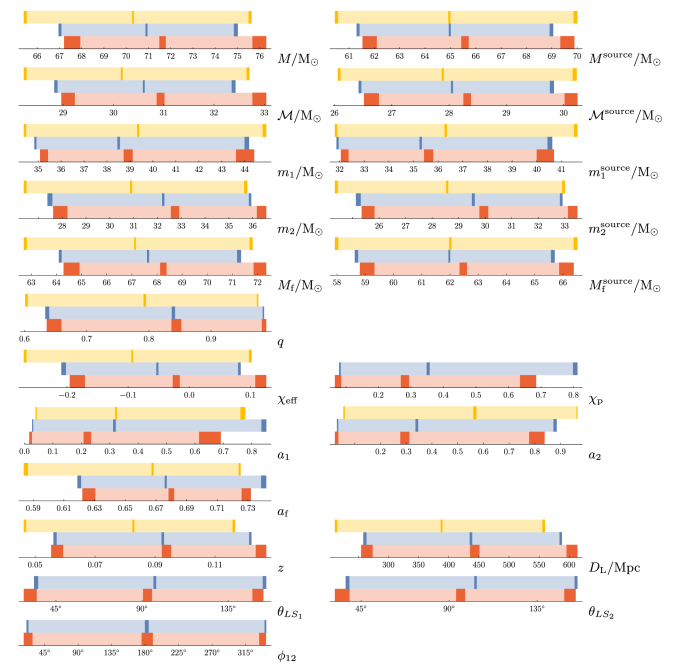
Comparison of parameter estimates for GW150914 using different waveform models. The bars show the 90% credible intervals, the dark bars show the uncertainty on the 5%, 50% and 95% quantiles from the finite number of posterior samples. The top bar is for the non-precessing EOBNR model, the middle is for the precessing IMRPhenom model, and the bottom is for the fully precessing EOBNR model. Figure 1 of the Precession Paper; see Figure 9 for a comparison of averaged EOBNR and IMRPhenom results, which we have used for our overall results.

We had used the difference between the EOBNR and IMRPhenom results to estimate potential systematic error from waveform modelling. Since the two precessing models are generally in better agreement, we have may have been too pessimistic here.

The main difference in results is that our new refined analysis gives tighter constraints on the spins. From the plot above you can see that the uncertainty for the spin magnitudes of the heavier black hole $a_1$ , the lighter black hole $a_2$ and the final black hole (resulting from the coalescence) $a_\mathrm{f}$ , are slightly narrower. This makes sense, as including the extra imprint from the full effects of precession gives us a bit more information about the spins. The plots below show the constraints on the spins from the two precessing waveforms: the distributions are more condensed with the new results.

Black hole spins estimated using precessing IMRPhenom and EOBNR waveforms

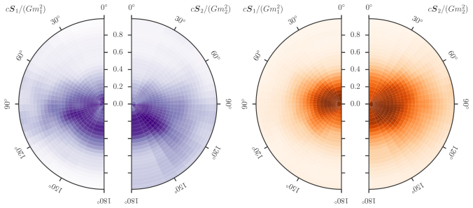
Comparison of orientations and magnitudes of the two component spins. The spin is perfectly aligned with the orbital angular momentum if the angle is 0. The left disk shows results using the precessing IMRPhenom model, the right using the precessing EOBNR model. In each, the distribution for the more massive black hole is on the left, and for the smaller black hole on the right. Adapted from Figure 5 of the Parameter Estimation Paper and Figure 4 of the Precession Paper.

In conclusion, this analysis had shown that included the full effects of precession do give slightly better estimates of the black hole spins. However, it is safe to trust the IMRPhenom results.

If you are looking for the best parameter estimates for GW150914, these results are better than the original results in the Parameter Estimation Paper. However, the O2 Catalogue Paper includes results using improved calibration and noise power spectral density estimation, as well as using precessing waveforms!

The Systematics Paper

Synopsis: Systematics Paper
Read this if: You want to know how parameter estimation could fare for future detections
Favourite part: There’s no need to panic yet

The Precession Paper highlighted how important it is to have good waveform templates. If there is an error in our templates, either because of modelling or because we are missing some physics, then our estimated parameters could be wrong—we would have a source of systematic error.

We know our waveform models aren’t perfect, so there must be some systematic error, the question is how much? From our analysis so far (such as the good agreement between different waveforms in the Precession Paper), we think that systematic error is less significant than the statistical uncertainty which is a consequence of noise in the detectors. In this paper, we try to quantify systematic error for GW150914-like systems.

To asses systematic errors, we analyse waveforms calculated by numerical relativity simulations into data around the time of GW150914. Numerical relativity exactly solves Einstein’s field equations (which govern general relativity), so results of these simulations give the most accurate predictions for the form of gravitational waves. As we know the true parameters for the injected waveforms, we can compare these to the results of our parameter estimation analysis to check for biases.

We use waveforms computed by two different codes: the Spectral Einstein Code (SpEC) and the Bifunctional Adaptive Mesh (BAM) code. (Don’t the names make them sound like such fun?) Most waveforms are injected into noise-free data, so that we know that any offset in estimated parameters is dues to the waveforms and not detector noise; however, we also tried a few injections into real data from around the time of GW150914. The signals are analysed using our standard set-up as used in the Parameter Estimation Paper (a couple of injections are also included in the Precession Paper, where they are analysed with the fully precessing EOBNR waveform to illustrate its accuracy).

The results show that in most cases, systematic errors from our waveform models are small. However, systematic errors can be significant for some orientations of precessing binaries. If we are looking at the orbital plane edge on, then there can be errors in the distance, the mass ratio and the spins, as illustrated below [bonus note]. Thankfully, edge-on binaries are quieter than face-on binaries, and so should make up only a small fraction of detected sources (GW150914 is most probably face off). Furthermore, biases are only significant for some polarization angles (an angle which describes the orientation of the detectors relative to the stretch/squash of the gravitational wave polarizations). Factoring this in, a rough estimate is that about 0.3% of detected signals would fall into the unlucky region where waveform biases are important.

Inclination dependence of parameter recovery

Parameter estimation results for two different GW150914-like numerical relativity waveforms for different inclinations and polarization angles. An inclination of $0^\circ$ means the binary is face on, $180^\circ$ means it face off, and an inclination around $90^\circ$ is edge on. The bands show the recovered 90% credible interval; the dark lines the median values, and the dotted lines show the true values. The (grey) polarization angle $\psi = 82^\circ$ was chosen so that the detectors are approximately insensitive to the $h_+$ polarization. Figure 4 of the Systematics Paper.

While it seems that we don’t have to worry about waveform error for GW150914, this doesn’t mean we can relax. Other systems may show up different aspects of waveform models. For example, our approximants only include the dominant modes (spherical harmonic decompositions of the gravitational waves). Higher-order modes have more of an impact in systems where the two black holes are unequal masses, or where the binary has a higher total mass, so that the merger and ringdown parts of the waveform are more important. We need to continue work on developing improved waveform models (or at least, including our uncertainty about them in our analysis), and remember to check for biases in our results!

The Numerical Relativity Comparison Paper

Synopsis: Numerical Relativity Comparison Paper
Read this if: You are really suspicious of our waveform models, or really like long tables or numerical data
Favourite part: We might one day have enough numerical relativity waveforms to do full parameter estimation with them

In the Precession Paper we discussed how important it was to have accurate waveforms; in the Systematics Paper we analysed numerical relativity waveforms to check the accuracy of our results. Since we do have numerical relativity waveforms, you might be wondering why we don’t just use these in our analysis? In this paper, we give it a go.

Our standard parameter-estimation code (LALInference) randomly hops around parameter space, for each set of parameters we generate a new waveform and see how this matches the data. This is an efficient way of exploring the parameter space. Numerical relativity waveforms are too computationally expensive to generate one each time we hop. We need a different approach.

The alternative, is to use existing waveforms, and see how each of them match. Each simulation gives the gravitational waves for a particular mass ratio and combination of spins, we can scale the waves to examine different total masses, and it is easy to consider what the waves would look like if measured at a different position (distance, inclination or sky location). Therefore, we can actually cover a fair range of possible parameters with a given set of simulations.

To keep things quick, the code averages over positions, this means we don’t currently get an estimate on the redshift, and so all the masses are given as measured in the detector frame and not as the intrinsic masses of the source.

The number of numerical relativity simulations is still quite sparse, so to get nice credible regions, a simple Gaussian fit is used for the likelihood. I’m not convinced that this capture all the detail of the true likelihood, but it should suffice for a broad estimate of the width of the distributions.

The results of this analysis generally agree with those from our standard analysis. This is a relief, but not surprising given all the other checks that we have done! It hints that we might be able to get slightly better measurements of the spins and mass ratios if we used more accurate waveforms in our standard analysis, but the overall conclusions are sound.

I’ve been asked if since these results use numerical relativity waveforms, they are the best to use? My answer is no. As well as potential error from the sparse sampling of simulations, there are several small things to be wary of.

We only have short numerical relativity waveforms. This means that the analysis only goes down to a frequency of $30~\mathrm{Hz}$ and ignores earlier cycles. The standard analysis includes data down to $20~\mathrm{Hz}$ , and this extra data does give you a little information about precession. (The limit of the simulation length also means you shouldn’t expect this type of analysis for the longer LVT151012 or GW151226 any time soon).
This analysis doesn’t include the effects of calibration uncertainty. There is some uncertainty in how to convert from the measured signal at the detectors’ output to the physical strain of the gravitational wave. Our standard analysis fold this in, but that isn’t done here. The estimates of the spin can be affected by miscalibration. (This paper also uses the earlier calibration, rather than the improved calibration of the O1 Binary Black Hole Paper).
Despite numerical relativity simulations producing waveforms which include all higher modes, not all of them are actually used in the analysis. More are included than in the standard analysis, so this will probably make negligible difference.

Finally, I wanted to mention one more detail, as I think it is not widely appreciated. The gravitational wave likelihood is given by an inner product

$\displaystyle L \propto \exp \left[- \int_{-\infty}^{\infty} \mathrm{d}f \frac{|s(f) - h(f)|^2}{S_n(f)} \right]$ ,

where $s(f)$ is the signal, $h(f)$ is our waveform template and $S_n(f)$ is the noise spectral density (PSD). These are the three things we need to know to get the right answer. This paper, together with the Precession Paper and the Systematics Paper, has been looking at error from our waveform models $h(f)$ . Uncertainty from the calibration of $s(f)$ is included in the standard analysis, so we know how to factor this in (and people are currently working on more sophisticated models for calibration error). This leaves the noise PSD $S_n(f)$ …

The noise PSD varies all the time, so it needs to be estimated from the data. If you use a different stretch of data, you’ll get a different estimate, and this will impact your results. Ideally, you would want to estimate from the time span that includes the signal itself, but that’s tricky as there’s a signal in the way. The analysis in this paper calculates the noise power spectral density using a different time span and a different method than our standard analysis; therefore, we expect some small difference in the estimated parameters. This might be comparable to (or even bigger than) the difference from switching waveforms! We see from the similarity of results that this cannot be a big effect, but it means that you shouldn’t obsess over small differences, thinking that they could be due to waveform differences, when they could just come from estimation of the noise PSD.

Lots of work is currently going into making sure that the numerator term $|s(f) - h(f)|^2$ is accurate. I think that the denominator $S_n(f)$ needs attention too. Since we have been kept rather busy, including uncertainty in PSD estimation will have to wait for a future set papers.

Bonus notes

Finches

100 bonus points to anyone who folds up the papers to make beaks suitable for eating different foods.

The right answer

Our current best estimate for the chirp mass (from the O2 Catalogue Paper) would be $31.2_{-1.5}^{+1.7} M_\odot$ . You need proper templates for the gravitational wave signal to calculate this. If you factor in the the gravitational wave gets redshifted (shifted to lower frequency by the expansion of the Universe), then the true chirp mass of the source system is $28.6_{-1.5}^{+1.6} M_\odot$ .

Formative experiences

My one undergraduate lecture on gravitational waves was the penultimate lecture of the fourth-year general relativity course. I missed this lecture, as I had a PhD interview (at the University of Birmingham). Perhaps if I had sat through it, my research career would have been different?

Good things come…

The computational expense of a waveform is important, as when we are doing parameter estimation, we calculate lots (tens of millions) of waveforms for different parameters to see how they match the data. Before O1, the task of using SEOBNRv3 for parameter estimation seemed quixotic. The first detection, however, was enticing enough to give it a try. It was a truly heroic effort by Vivien Raymond and team that produced these results—I am slightly suspicious the Vivien might actually be a wizard.

GW150914 is a short signal, meaning it is relatively quick to analyse. Still, it required us using all the tricks at our disposal to get results in a reasonable time. When it came time to submit final results for the Discovery Paper, we had just about 1,000 samples from the posterior probability distribution for the precessing EOBNR waveform. For comparison, we had over 45,000 sample for the non-precessing EOBNR waveform. 1,000 samples isn’t enough to accurately map out the probability distributions, so we decided to wait and collect more samples. The preliminary results showed that things looked similar, so there wouldn’t be a big difference in the science we could do. For the Precession Paper, we finally collected 2,700 samples. This is still a relatively small number, so we carefully checked the uncertainty in our results due to the finite number of samples.

The Precession Paper has shown that it is possible to use the precessing EOBNR for parameter estimation, but don’t expect it to become the norm, at least until we have a faster implementation of it. Vivien is only human, and I’m sure his family would like to see him occasionally.

Parameter key

In case you are wondering what all the symbols in the results plots stand for, here are their usual definitions. First up, the various masses

$m_1$ —the mass of the heavier black hole, sometimes called the primary black hole;
$m_2$ —the mass of the lighter black hole, sometimes called the secondary black hole;
$M$ —the total mass of the binary, $M = m_1 + m_2$ ;
$M_\mathrm{f}$ —the mass of the final black hole (after merger);
$\mathcal{M}$ —the chirp mass, the combination of the two component masses which sets how the binary inspirals together;
$q$ —the mass ratio, $q = m_1/m_2 \leq 1$ . Confusingly, numerical relativists often use the opposite convention $q = m_2/m_1 \geq 1$ (which is why the Numerical Relativity Comparison Paper discusses results in terms of $1/q$ : we can keep the standard definition, but all the numbers are numerical relativist friendly).

A superscript “source” is sometimes used to distinguish the actual physical masses of the source from those measured by the detector which have been affected by cosmological redshift. The measured detector-frame mass is $m = (1 + z) m^\mathrm{source}$ , where $m^\mathrm{source}$ is the true, redshift-corrected source-frame mass and $z$ is the redshift. The mass ratio $q$ is independent of the redshift. On the topic of redshift, we have

$z$ —the cosmological redshift ( $z = 0$ would be now);
$D_\mathrm{L}$ —the luminosity distance.

The luminosity distance sets the amplitude of the signal, as does the orientation which we often describe using

$\iota$ —the inclination, the angle between the line of sight and the orbital angular momentum ( $\boldsymbol{L}$ ). This is zero for a face-on binary.
$\theta_{JN}$ —the angle between the line of sight ( $\boldsymbol{N}$ ) and the total angular momentum of the binary ( $\boldsymbol{J}$ ); this is approximately equal to the inclination, but is easier to use for precessing binaries.

As well as masses, black holes have spins

$a_1$ —the (dimensionless) spin magnitude of the heavier black hole, which is between $0$ (no spin) and $1$ (maximum spin);
$a_2$ —the (dimensionless) spin magnitude of the lighter black hole;
$a_\mathrm{f}$ —the (dimensionless) spin magnitude of the final black hole;
$\chi_\mathrm{eff}$ —the effective inspiral spin parameter, a combinations of the two component spins which has the largest impact on the rate of inspiral (think of it as the spin equivalent of the chirp mass);
$\chi_\mathrm{p}$ —the effective precession spin parameter, a combination of spins which indicate the dominant effects of precession, it’s $0$ for no precession and $1$ for maximal precession;
$\theta_{LS_1}$ —the primary tilt angle, the angle between the orbital angular momentum and the heavier black holes spin ( $\boldsymbol{S_1}$ ). This is zero for aligned spin.
$\theta_{LS_2}$ —the secondary tilt angle, the angle between the orbital angular momentum and the lighter black holes spin ( $\boldsymbol{S_2}$ ).
$\phi_{12}$ —the angle between the projections of the two spins on the orbital plane.

The orientation angles change in precessing binaries (when the spins are not perfectly aligned or antialigned with the orbital angular momentum), so we quote values at a reference time corresponding to when the gravitational wave frequency is $20~\mathrm{Hz}$ . Finally (for the plots shown here)

$\psi$ —the polarization angle, this is zero when the detector arms are parallel to the $h_+$ polarization’s stretch/squash axis.

For more detailed definitions, check out the Parameter Estimation Paper or the LALInference Paper.

Parameter estimation for binary neutron-star coalescences with realistic noise during the Advanced LIGO era

May 14, 2015February 9, 2020 / CPLB / Leave a comment

The first observing run (O1) of Advanced LIGO is nearly here, and with it the prospect of the first direct detection of gravitational waves. That’s all wonderful and exciting (far more exciting than a custard cream or even a chocolate digestive), but there’s a lot to be done to get everything ready. Aside from remembering to vacuum the interferometer tubes and polish the mirrors, we need to see how the data analysis will work out. After all, having put so much effort into the detector, it would be shame if we couldn’t do any science with it!

Parameter estimation

Since joining the University of Birmingham team, I’ve been busy working on trying to figure out how well we can measure things using gravitational waves. I’ve been looking at binary neutron star systems. We expect binary neutron star mergers to be the main source of signals for Advanced LIGO. We’d like to estimate how massive the neutron stars are, how fast they’re spinning, how far away they are, and where in the sky they are. Just published is my first paper on how well we should be able to measure things. This took a lot of hard work from a lot of people, so I’m pleased it’s all done. I think I’ve earnt a celebratory biscuit. Or two.

When we see something that looks like it could be a gravitational wave, we run code to analyse the data and try to work out the properties of the signal. Working out some properties is a bit trickier than others. Sadly, we don’t have an infinite number of computers, so it means it can take a while to get results. Much longer than the time to eat a packet of Jaffa Cakes…

The fastest algorithm we have for binary neutron stars is BAYESTAR. This takes the same time as maybe eating one chocolate finger. Perhaps two, if you’re not worried about the possibility of choking. BAYESTAR is fast as it only estimates where the source is coming from. It doesn’t try to calculate a gravitational-wave signal and match it to the detector measurements, instead it just looks at numbers produced by the detection pipeline—the code that monitors the detectors and automatically flags whenever something interesting appears. As far as I can tell, you give BAYESTAR this information and a fresh cup of really hot tea, and it uses Bayes’ theorem to work out how likely it is that the signal came from each patch of the sky.

To work out further details, we need to know what a gravitational-wave signal looks like and then match this to the data. This is done using a different algorithm, which I’ll refer to as LALInference. (As names go, this isn’t as cool as SKYNET). This explores parameter space (hopping between different masses, distances, orientations, etc.), calculating waveforms and then working out how well they match the data, or rather how likely it is that we’d get just the right noise in the detector to make the waveform fit what we observed. We then use another liberal helping of Bayes’ theorem to work out how probable those particular parameter values are.

It’s rather difficult to work out the waveforms, but some our easier than others. One of the things that makes things trickier is adding in the spins of the neutron stars. If you made a batch of biscuits at the same time you started a LALInference run, they’d still be good by the time a non-spinning run finished. With a spinning run, the biscuits might not be quite so appetising—I generally prefer more chocolate than penicillin on my biscuits. We’re working on speeding things up (if only to prevent increased antibiotic resistance).

In this paper, we were interested in what you could work out quickly, while there’s still chance to catch any explosion that might accompany the merging of the neutron stars. We think that short gamma-ray bursts and kilonovae might be caused when neutron stars merge and collapse down to a black hole. (I find it mildly worrying that we don’t know what causes these massive explosions). To follow-up on a gravitational-wave detection, you need to be able to tell telescopes where to point to see something and manage this while there’s still something that’s worth seeing. This means that using spinning waveforms in LALInference is right out, we just use BAYESTAR and the non-spinning LALInference analysis.

What we did

To figure out what we could learn from binary neutron stars, we generated a large catalogue of fakes signals, and then ran the detection and parameter-estimation codes on this to see how they worked. This has been done before in The First Two Years of Electromagnetic Follow-Up with Advanced LIGO and Virgo which has a rather delicious astrobites write-up. Our paper is the sequel to this (and features most of the same cast). One of the differences is that The First Two Years assumed that the detectors were perfectly behaved and had lovely Gaussian noise. In this paper, we added in some glitches. We took some real data™ from initial LIGO’s sixth science run and stretched this so that it matches the sensitivity Advanced LIGO is expected to have in O1. This process is called recolouring [bonus note]. We now have fake signals hidden inside noise with realistic imperfections, and can treat it exactly as we would real data. We ran it through the detection pipeline, and anything which was flagged as probably being a signal (we used a false alarm rate of once per century), was analysed with the parameter-estimation codes. We looked at how well we could measure the sky location and distance of the source, and the masses of the neutron stars. It’s all good practice for O1, when we’ll be running this analysis on any detections.

What we found

The flavour of noise (recoloured or Gaussian) makes no difference to how well we can measure things on average.
Sky-localization in O1 isn’t great, typically hundreds of square degrees (the median 90% credible region is 632 deg²), for comparison, the Moon is about a fifth of a square degree. This’ll make things interesting for the people with telescopes.
Probability that of a gravitational-wave signal coming from different points on the sky. The darker the red, the higher the probability. The star indicates the true location. This is one of the worst localized events from our study for O1. You can find more maps in the data release (including 3D versions), this is Figure 6 of Berry et al. (2015).
BAYESTAR does just as well as LALInference, despite being about 2000 times faster.
Sky localization (the size of the patch of the sky that we’re 90% sure contains the source location) varies with the signal-to-noise ratio (how loud the signal is). The approximate best fit is $\log_{10}(\mathrm{CR}_{0.9}/\mathrm{deg^2}) \approx -2 \log_{10}(\varrho) +5.06$ , where $\mathrm{CR}_{0.9}$ is the 90% sky area and $\varrho$ is the signal-to-noise ratio. The results for BAYESTAR and LALInference agree, as do the results with Gaussian and recoloured noise. This is Figure 9 of Berry et al. (2015).
We can’t measure the distance too well: the median 90% credible interval divided by the true distance (which gives something like twice the fractional error) is 0.85.
Because we don’t include the spins of the neutron stars, we introduce some error into our mass measurements. The chirp mass, a combination of the individual masses that we’re most sensitive to [bonus note], is still reliably measured (the median offset is 0.0026 of the mass of the Sun, which is tiny), but we’ll have to wait for the full spinning analysis for individual masses.
Fraction of events with difference between the mean estimated and true chirp mass smaller than a given value. There is an error because we are not including the effects of spin, but this is small. Again, the type of noise makes little difference. This is Figure 15 of Berry et al. (2015).

There’s still some work to be done before O1, as we need to finish up the analysis with waveforms that include spin. In the mean time, our results are all available online for anyone to play with.

arXiv: 1411.6934 [astro-ph.HE]
Journal: Astrophysical Journal; 904(2):114(24); 2015
Data release: The First Two Years of Electromagnetic Follow-Up with Advanced LIGO and Virgo
Favourite colour: Blue. No, yellow…

Notes

The colour of noise: Noise is called white if it doesn’t have any frequency dependence. We made ours by taking some noise with initial LIGO’s frequency dependence (coloured noise), removing the frequency dependence (making it white), and then adding in the frequency dependence of Advanced LIGO (recolouring it).

The chirp mass: Gravitational waves from a binary system depend upon the masses of the components, we’ll call these $m_1$ and $m_2$ . The chirp mass is a combination these that we can measure really well, as it determines the most significant parts of the shape of the gravitational wave. It’s given by

$\displaystyle \mathcal{M} = \frac{m_1^{3/5} m_2^{3/5}}{(m_1 + m_2)^{1/5}}$ .

We get lots of good information on the chirp mass, unfortunately, this isn’t too useful for turning back into the individual masses. For that we next extra information, for example the mass ratio $m_2/m_1$ . We can get this from less dominant parts of the waveform, but it’s not typically measured as precisely as the chirp mass, so we’re often left with big uncertainties.

Life as a binary

Gravitational-wave observations

Results

Bonus notes

Channel selection

Kick distribution

The likelihood

Interpretation of the Fisher information matrix

Share this:

Bonus notes

Detector engineering

Parameter estimation rota

Alerts and follow-up

Virgo?

Journal

Share this:

Discovery

Science

Summary

Bonus notes

Inbox zero

Worst case scenario

Parameter estimation rota

Especially made

Share this:

The papers

13. The Basic Physics Paper

14. The Precession Paper

15. The Systematics Paper

16. The Numerical Relativity Comparison Paper

The Basic Physics Paper

The Precession Paper

The Systematics Paper

The Numerical Relativity Comparison Paper

Bonus notes

Finches

The right answer

Formative experiences

Good things come…

Parameter key

Share this:

Parameter estimation

What we did

What we found

Notes

Share this: