One of the great discoveries that came with our first observation of gravitational waves was that black holes can merge—two black holes in a binary can come together and form a bigger black hole. This had long been predicted, but never before witnessed. If black holes can merge once, can they go on to merge again? In this paper, we calculated how to identify a binary containing a second-generation black hole formed in a merger.
Merging black holes
Black holes have two important properties: their mass and their spin. When two black holes merge, the resulting black hole has:
A mass which is almost as big as the sum of the masses of its two parents. It is a little less (about 5%) as some of the energy is radiated away as gravitational waves.
A spin which is around 0.7. This is set by the angular momentum of the two black holes as they plunge in together. For equal-mass black holes, the orbit of the two black holes will give about enough angular momentum for the final black hole to be about 0.7. The spins of the two parent black holes will cause a bit a variation around this, depending upon the orientations of their spins. For more unequal mass binaries, the spin of the larger parent black hole becomes more important.
To look for second-generation (or higher) black holes formed in mergers, we need to look for more massive black holes with spins of about 0.7 [bonus note].
Combining black holes. The result of a merger is a larger black hole with significant spin. From Dawn Finney.
The difficult bit here is that we don’t know the distribution of masses and spins of the initial first-generation black holes. What is they naturally form with spins of 0.7? How can you tell if a black hole is unexpectedly large if you don’t know what sizes to expect? With the discovery of the 10 binary black holes found in our first and second observing runs, we are able to start making inferences about the properties of black holes—using these measurements of the population, we can estimate how probable it is that a binary contains a second generation black hole versus containing two first generation black hole.
GW170729
Amongst the black holes observed in O1 and O2, the source of GW170729 stands out. It is both the most massive, and one of only two systems (the other being GW151226) showing strong evidence for spin. This got me wondering if it could be a second-generation system? The high mass would be explained as we have a second-generation black hole, and the spin is larger than usual as a spin 0.7 sticks out.
Chase Kimball worked out the relative probability of getting a system with a given chirp mass and effective inspiral spin for a binary with a second-generation black hole verses a binary with only first-generation black holes. We worked in terms of chirp mass and effective inspiral spin, as these are the properties we measure well from a gravitational-wave signal.
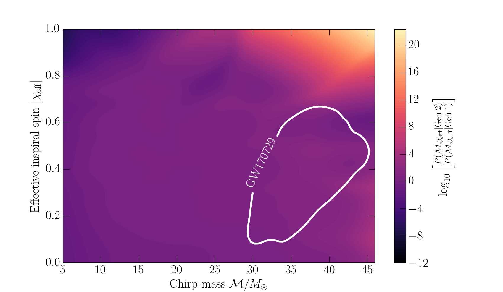
Relative likelihood of a binary black hole being second-generation versus first-generation for different values of the chirp mass and the magnitude of the effective inspiral spin. The white contour gives the 90% credible area for GW170729. Figure 1 of Kimball et al. (2019).
The plot above shows the relative probabilities. Yellow indicate chirp mass and effective inspiral spins which are more likely with second-generation systems, while dark purple indicates values more likely with first-generation systems.. The first thing I realised was my idea about the spin was off. We expect binaries with second-generation black holes to be formed dynamically. Following the first merger, the black hole wander around until it gets close enough to form a new binary with a new black hole. For dynamically formed binaries the spins should be randomly distributed. This means that there’s only a small probability of having a spin aligned with the orbital angular momentum as measured for GW170729. Most of the time, you’d measure an effective inspiral spin of around zero.
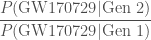
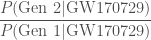
Since we don’t know exactly the chirp mass and effective inspiral spin for GW170729, we have to average over our uncertainty. That gives the ratio of the probability of observing GW170729 given a second-generation source, verses given a first-generation source. Using different inferred black hole populations (for example, ones inferred including and excluding GW170729), we find ratios of between 0.2 (meaning the first-generation origin is more likely) and 16 (meaning second generation is more likely). The results change significantly as the result is sensitive to the maximum mass of a black hole. If we include GW170729 in our population inference for first-generation systems, the maximum mass goes up, and it’s easier to explain the system as first-generation (as you’d expect).
Before you place your bets, there is one more piece to the calculation. We have calculated the relative probabilities of the observed properties assuming either first-generation black holes or a second-generation black hole, but we have not folded in the relative rates of mergers [bonus note]. We expect first-generation only binaries to be more common than ones containing second generation black holes. In simulations of globular clusters, at most about 20% of merging binaries are with second-generation black holes. For binaries not in an environment like a globular cluster (where there are lots of nearby black holes to grab), we expect the fraction of second-generation black holes in binaries to be basically zero. Therefore, on balance we have at best a weak preference for a second-generation black hole and most probably just two first-generation black holes in GW170729’s source, despite its large mass.
Verdict
What we have learnt from this calculation is that it seems that all of the first 10 binary black holes contain only first-generation black holes. It is safe to infer the properties of first-generation black holes from these observations. Detecting second-generation black holes requires knowledge of this distribution, and crucially if there is a maximum mass. As we get more detection, we’ll be able to pin this down. There is still a lot to learn about the full black hole family.
If you’d like to understand our calculation, the paper is extremely short. It is therefore an excellent paper to bring to journal club if you are a PhD student who forgot you were presenting this week…
I was asked how we could tell if the black holes we were seeing were themselves the results of mergers back in 2016 when I was giving a talk to the Carolian Astronomical Society. It was a good question. I explained about the masses and spins, but I didn’t think about how to actually do the analysis to infer if we had a merger. I now make a note to remember any questions I’m asked, as they can be good inspiration for projects!
Bayes factor and odds ratio
The quantity we work out in the paper is the Bayes factor for a second-generation system verses a first-generation one
which gives the betting odds for the two scenarios. The convert the Bayes factor into an odds ratio we need the prior odds
.
We’re currently working on a better way to fold these pieces together.
1000 words
As this was a quick calculation, we thought it would be a good paper to be a Research Note. Research Notes are limited to 1000 words, which is a tough limit. We carefully crafted the document, using as many word-saving measures (such as abbreviations), as we could. We made it to the limit by our counting, only to submit and find that we needed to share another 100 off! Fortunately, the arXiv [bonus bonus note] is more forgiving, so you can read our more relaxed (but still delightfully short) version there. It’s the one I’d recommend.
arXiv
For those reading who are not professional physicists, the arXiv (pronounced archive, as the X is really the Greek letter chi χ) is a preprint server. It where physicists can post version of their papers ahead of publication. This allows sharing of results earlier (both good as it can take a while to get a final published paper, and because you can get feedback before finalising a paper), and, vitally, for free. Most published papers require a subscription to read. Fine if you’re at a university, not so good otherwise. The arXiv allows anyone to read the latest research. Admittedly, you have to be careful, as not everything on the arXiv will make it through peer review, and not everyone will update their papers to reflect the published version. However, I think the arXiv is a very good thing™. There are few things I can think of which have benefited modern science as much. I would 100% support those behind the arXiv receiving a Nobel Prize, as I think it has had just as a significant impact on the development of the field as the discovery of dark matter, understanding nuclear fission, or deducing the composition of the Sun.
Advanced LIGO and Advanced Virgo have detected their first binary neutron star inspiral. Remarkably, this event was observed not just with gravitational waves, but also across the electromagnetic spectrum, from gamma-rays to radio. This discovery confirms the theory that binary neutron star mergers are the progenitors of short gamma-ray bursts and kilonovae, and may be the primary source of heavy elements like gold.
In this post, I’ll go through some of the story of GW170817. As for GW150914, I’ll write another post on the more technical details of our papers, once I’ve had time to catch up on sleep.
Discovery
The second observing run (O2) of the advanced gravitational-wave detectors started on 30 November 2016. The first detection came in January—GW170104. I was heavily involved in the analysis and paper writing for this. We finally finished up in June, at which point I was thoroughly exhausted. I took some time off in July [bonus note], and was back at work for August. With just one month left in the observing run, it would all be downhill from here, right?
August turned out to be the lava-filled, super-difficult final level of O2. As we have now announced, on August 14, we detected a binary black hole coalescence—GW170814. This was the first clear detection including Virgo, giving us superb sky localization. This is fantastic for astronomers searching for electromagnetic counterparts to our gravitational-wave signals. There was a flurry of excitement, and we thought that this was a fantastic conclusion to O2. We were wrong, this was just the save point before the final opponent. On August 17, we met the final, fire-ball throwing boss.
Text messages from our gravitational-wave candidate event database GraceDB. The final message is for GW170817, or as it was known at the time, G298048. It certainly caught my attention. The messages above are for GW170814, that was picked up multiple times by our search algorithms. It was a busy week.
At 1:58 pm BST my phone buzzed with a text message, an automated alert of a gravitational-wave trigger. I was obviously excited—I recall that my exact thoughts were “What fresh hell is this?” I checked our online event database and saw that it was a single-detector trigger, it was only seen by our Hanford instrument. I started to relax, this was probably going to turn out to be a glitch. The template masses, were low, in the neutron star range, not like the black holes we’ve been finding. Then I saw the false alarm rate was better than one in 9000 years. Perhaps it wasn’t just some noise after all—even though it’s difficult to estimate false alarm rates accurately online, as especially for single-detector triggers, this was significant! I kept reading. Scrolling down the page there was an external coincident trigger, a gamma-ray burst (GRB 170817A) within a couple of seconds…
Short gamma-ray bursts are some of the most powerful explosions in the Universe. I’ve always found it mildly disturbing that we didn’t know what causes them. The leading theory has been that they are the result of two neutron stars smashing together. Here seemed to be the proof.
The rapid response call was under way by the time I joined. There was a clear chirp in Hanford, you could be see it by eye! We also had data from Livingston and Virgo too. It was bad luck that they weren’t folded into the online alert. There had been a drop out in the data transfer from Italy to the US, breaking the flow for Virgo. In Livingston, there was a glitch at the time of the signal which meant the data wasn’t automatically included in the search. My heart sank. Glitches are common—check out Gravity Spy for some examples—so it was only a matter of time until one overlapped with a signal [bonus note], and with GW170817 being such a long signal, it wasn’t that surprising. However, this would complicate the analysis. Fortunately, the glitch is short and the signal is long (if this had been a high-mass binary black hole, things might not have been so smooth). We were able to exorcise the glitch. A preliminary sky map using all three detectors was sent out at 12:54 am BST. Not only did we defeat the final boss, we did a speed run on the hard difficulty setting first time [bonus note].
Spectrogram of Livingston data showing part of GW170817’s chirp (which sweeps upward in frequncy) as well as the glitch (the big blip at about ). The lower panel shows how we removed the glitch: the grey line shows gating window that was applied for preliminary results, to zero the affected times, the blue shows a fitted model of the glitch that was subtracted for final results. You can clearly see the chirp well before the glitch, so there’s no danger of it being an artefect of the glitch. Figure 2 of the GW170817 Discovery Paper
The three-detector sky map provided a great localization for the source—this preliminary map had a 90% area of ~30 square degrees. It was just in time for that night’s observations. The plot below shows our gravitational-wave localizations in green—the long band is without Virgo, and the smaller is with all three detectors—as with GW170814, Virgo makes a big difference. The blue areas are the localizations from Fermi and INTEGRAL, the gamma-ray observatories which measured the gamma-ray burst. The inset is something new…
Localization of the gravitational-wave, gamma-ray, and optical signals. The main panel shows initial gravitational-wave 90% areas in green (with and without Virgo) and gamma-rays in blue (the IPN triangulation from the time delay between Fermi and INTEGRAL, and the Fermi GBM localization). The inset shows the location of the optical counterpart (the top panel was taken 10.9 hours after merger, the lower panel is a pre-merger reference without the transient). Figure 1 of the Multimessenger Astronomy Paper.
That night, the discoveries continued. Following up on our sky location, an optical counterpart (AT 2017gfo) was found. The source is just on the outskirts of galaxy NGC 4993, which is right in the middle of the distance range we inferred from the gravitational wave signal. At around 40 Mpc, this is the closest gravitational wave source.
After this source was reported, I think about every single telescope possible was pointed at this source. I think it may well be the most studied transient in the history of astronomy. I think there are ~250 circulars about follow-up. Not only did we find an optical counterpart, but there was emission in X-ray and radio. There was a delay in these appearing, I remember there being excitement at our Collaboration meeting as the X-ray emission was reported (there was a lack of cake though).
The figure below tries to summarise all the observations. As you can see, it’s a mess because there is too much going on!
The timeline of observations of GW170817’s source. Shaded dashes indicate times when information was reported in a Circular. Solid lines show when the source was observable in a band: the circles show a comparison of brightnesses for representative observations. Figure 2 of the Multimessenger Astronomy Paper.
The observations paint a compelling story. Two neutron stars insprialled together and merged. Colliding two balls of nuclear density material at around a third of the speed of light causes a big explosion. We get a jet blasted outwards and a gamma-ray burst. The ejected, neutron-rich material decays to heavy elements, and we see this hot material as a kilonova [bonus material]. The X-ray and radio may then be the afterglow formed by the bubble of ejected material pushing into the surrounding interstellar material.
Science
What have we learnt from our results? Here are some gravitational wave highlights.
We measure several thousand cycles from the inspiral. It is the most beautiful chirp! This is the loudest gravitational wave signal yet found, beating even GW150914. GW170817 has a signal-to-noise ratio of 32, while for GW150914 it is just 24.
Time–frequency plots for GW170104 as measured by Hanford, Livingston and Virgo. The signal is clearly visible in the two LIGO detectors as the upward sweeping chirp. It is not visible in Virgo because of its lower sensitivity and the source’s position in the sky. The Livingston data have the glitch removed. Figure 1 of the GW170817 Discovery Paper.
The signal-to-noise ratios in the Hanford, Livingston and Virgo were 19, 26 and 2 respectively. The signal is quiet in Virgo, which is why you can’t spot it by eye in the plots above. The lack of a clear signal is really useful information, as it restricts where on the sky the source could be, as beautifully illustrated in the video below.
While we measure the inspiral nicely, we don’t detect the merger: we can’t tell if a hypermassive neutron star is formed or if there is immediate collapse to a black hole. This isn’t too surprising at current sensitivity, the system would basically need to convert all of its energy into gravitational waves for us to see it.
From measuring all those gravitational wave cycles, we can measure the chirp mass stupidly well. Unfortunately, converting the chirp mass into the component masses is not easy. The ratio of the two masses is degenerate with the spins of the neutron stars, and we don’t measure these well. In the plot below, you can see the probability distributions for the two masses trace out bananas of roughly constant chirp mass. How far along the banana you go depends on what spins you allow. We show results for two ranges: one with spins (aligned with the orbital angular momentum) up to 0.89, the other with spins up to 0.05. There’s nothing physical about 0.89 (it was just convenient for our analysis), but it is designed to be agnostic, and above the limit you’d plausibly expect for neutron stars (they should rip themselves apart at spins of ~0.7); the lower limit of 0.05 should safely encompass the spins of the binary neutron stars (which are close enough to merge in the age of the Universe) we have estimated from pulsar observations. The masses roughly match what we have measured for the neutron stars in our Galaxy. (The combinations at the tip of the banana for the high spins would be a bit odd).
Estimated masses for the two neutron stars in the binary. We show results for two different spin limits, is the component of the spin aligned with the orbital angular momentum. The two-dimensional shows the 90% probability contour, which follows a line of constant chirp mass. The one-dimensional plot shows individual masses; the dotted lines mark 90% bounds away from equal mass. Figure 4 of the GW170817 Discovery Paper.
If we were dealing with black holes, we’d be done: they are only described by mass and spin. Neutron stars are more complicated. Black holes are just made of warped spacetime, neutron stars are made of delicious nuclear material. This can get distorted during the inspiral—tides are raised on one by the gravity of the other. These extract energy from the orbit and accelerate the inspiral. The tidal deformability depends on the properties of the neutron star matter (described by its equation of state). The fluffier a neutron star is, the bigger the impact of tides; the more compact, the smaller the impact. We don’t know enough about neutron star material to predict this with certainty—by measuring the tidal deformation we can learn about the allowed range. Unfortunately, we also didn’t yet have good model waveforms including tides, so for to start we’ve just done a preliminary analysis (an improved analysis was done for the GW170817 Properties Paper). We find that some of the stiffer equations of state (the ones which predict larger neutron stars and bigger tides) are disfavoured; however, we cannot rule out zero tides. This means we can’t rule out the possibility that we have found two low-mass black holes from the gravitational waves alone. This would be an interesting discovery; however, the electromagnetic observations mean that the more obvious explanation of neutron stars is more likely.
From the gravitational wave signal, we can infer the source distance. Combining this with the electromagnetic observations we can do some cool things.
First, the gamma ray burst arrived at Earth 1.7 seconds after the merger. 1.7 seconds is not a lot of difference after travelling something like 85–160 million years (that’s roughly the time since the Cretaceous or Late Jurassic periods). Of course, we don’t expect the gamma-rays to be emitted at exactly the moment of merger, but allowing for a sensible range of emission times, we can bound the difference between the speed of gravity and the speed of light. In general relativity they should be the same, and we find that the difference should be no more than three parts in .
Second, we can combine the gravitational wave distance with the redshift of the galaxy to measure the Hubble constant, the rate of expansion of the Universe. Our best estimates for the Hubble constant, from the cosmic microwave background and from supernova observations, are inconsistent with each other (the most recent supernova analysis only increase the tension). Which is awkward. Gravitational wave observations should have different sources of error and help to resolve the difference. Unfortunately, with only one event our uncertainties are rather large, which leads to a diplomatic outcome.
Posterior probability distribution for the Hubble constant inferred from GW170817. The lines mark 68% and 95% intervals. The coloured bands are measurements from the cosmic microwave background (Planck) and supernovae (SHoES). Figure 1 of the Hubble Constant Paper.
Finally, we can now change from estimating upper limits on binary neutron star merger rates to estimating the rates! We estimate the merger rate density is in the range (assuming a uniform of neutron star masses between one and two solar masses). This is surprisingly close to what the Collaboration expected back in 2010: a rate of between and , with a realistic rate of . This means that we are on track to see many more binary neutron stars—perhaps one a week at design sensitivity!
Summary
Advanced LIGO and Advanced Virgo observed a binary neutron star insprial. The rest of the astronomical community has observed what happened next (sadly there are no neutrinos). This is the first time we have such complementary observations—hopefully there will be many more to come. There’ll be a huge number of results coming out over the following days and weeks. From these, we’ll start to piece together more information on what neutron stars are made of, and what happens when you smash them together (take that particle physicists).
Also: I’m exhausted, my inbox is overflowing, and I will have far too many papers to read tomorrow.
If you’re looking for the most up-to-date results regarding GW170817, check out the O2 Catalogue Paper.
Bonus notes
Inbox zero
Over my vacation I cleaned up my email. I had a backlog starting around September 2015. I think there were over 6000 which I sorted or deleted. I had about 20 left to deal with when I got back to work. GW170817 undid that. Despite doing my best to keep up, there are over a 1000 emails in my inbox…
Worst case scenario
Around the start of O2, I was asked when I expected our results to be public. I said it would depend upon what we found. If it was only high-mass black holes, those are quick to analyse and we know what to do with them, so results shouldn’t take long, now we have the first few out of the way. In this case, perhaps a couple months as we would have been generating results as we went along. However, the worst case scenario would be a binary neutron star overlapping with non-Gaussian noise. Binary neutron stars are more difficult to analyse (they are longer signals, and there are matter effects to worry about), and it would be complicated to get everyone to be happy with our results because we were doing lots of things for the first time. Obviously, if one of these happened at the end of the run, there’d be quite a delay…
I think I got that half-right. We’re done amazingly well analysing GW170817 to get results out in just two months, but I think it will be a while before we get the full O2 set of results out, as we’ve been neglecting otherthings (you’ll notice we’ve not updated our binary black hole merger rate estimate since GW170104, nor given detailed results for testing general relativity with the more recent detections).
At the time of the GW170817 alert, I was working on writing a research proposal. As part of this, I was explaining why it was important to continue working on gravitational-wave parameter estimation, in particular how to deal with non-Gaussian or non-stationary noise. I think I may be a bit of a jinx. For GW170817, the glitch wasn’t a big problem, these type of blips can be removed. I’m more concerned about the longer duration ones, which are less easy to separate out from background noise. Don’t say I didn’t warn you in O3.
Parameter estimation rota
The duty of analysing signals to infer their source properties was divided up into shifts for O2. On January 4, the time of GW170104, I was on shift with my partner Aaron Zimmerman. It was his first day. Having survived that madness, Aaron signed back up for the rota. Can you guess who was on shift for the week which contained GW170814 and GW170817? Yep, Aaron (this time partnered with the excellent Carl-Johan Haster). Obviously, we’ll need to have Aaron on rota for the entirety of O3. In preparation, he has already started on paper drafting
Methods Section: Chained ROTA member to a terminal, ignored his cries for help. Detections followed swiftly.
Especially made
The lightest elements (hydrogen, helium and lithium) we made during the Big Bang. Stars burn these to make heavier elements. Energy can be released up to around iron. Therefore, heavier elements need to be made elsewhere, for example in the material ejected from supernova or (as we have now seen) neutron star mergers, where there are lots of neutrons flying around to be absorbed. Elements (like gold and platinum) formed by this rapid neutron capture are known as r-process elements, I think because they are beloved by pirates.
A couple of weeks ago, the Nobel Prize in Physics was announced for the observation of gravitational waves. In December, the laureates will be presented with a gold (not chocolate) medal. I love the idea that this gold may have come from merging neutron stars.
Here’s one we made earlier. Credit: Associated Press/F. Vergara
On 14 August 2017 a gravitational wave signal (GW170814), originating from the coalescence of a binary black hole system, was observed by the global gravitational-wave observatory network of the two Advanced LIGO detectors and Advanced Virgo. That’s right, Virgo is in the game!
Very few things excite me like unlocking a new character in Smash Bros. A new gravitational wave observatory might come close.
Advanced Virgo joined O2, the second observing run of the advanced detector era, on 1 August. This was a huge achievement. It has not been an easy route commissioning the new detector—it never ceases to amaze me how sensitive these machines are. Together, Advanced Virgo (near Pisa) and the two Advanced LIGO detectors (in Livingston and Hanford in the US) would take data until the end of O2 on 25 August.
On 14 August, we found a signal. A signal that was observable in all three detectors [bonus note]. Virgo is less sensitive than the LIGO instruments, so there is no impressive plot that shows something clearly popping out, but the Virgo data do complement the LIGO observations, indicating a consistent signal in all three detectors [bonus note].
A cartoon of three different ways to visualise GW170814 in the three detectors. These take a bit of explaining. The top panel shows the signal-to-noise ratio the search template that matched GW170814. They peak at the time corresponding to the merger. The peaks are clear in Hanford and Livingston. The peak in Virgo is less exceptional, but it matches the expected time delay and amplitude for the signal. The middle panels show time–frequency plots. The upward sweeping chirp is visible in Hanford and Livingston, but less so in Virgo as it is less sensitive. The plot is zoomed in so that its possible to pick out the detail in Virgo, but the chirp is visible for a longer stretch of time than plotted in Livingston. The bottom panel shows whitened and band-passed strain data, together with the 90% region of the binary black hole templates used to infer the parameters of the source (the narrow dark band), and an unmodelled, coherent reconstruction of the signal (the wider light band) . The agreement between the templates and the reconstruction is a check that the gravitational waves match our expectations for binary black holes. The whitening of the data mirrors how we do the analysis, by weighting noise at different frequency by an estimate of their typical fluctuations. The signal does certainly look like the inspiral, merger and ringdown of a binary black hole. Figure 1 of the GW170814 Paper.
The signal originated from the coalescence of two black holes. GW170814 is thus added to the growing family of GW150914, LVT151012, GW151226 and GW170104.
GW170814 most closely resembles GW150914 and GW170104 (perhaps there’s something about ending with a 4). If we compare the masses of the two component black holes of the binary ( and ), and the black hole they merge to form (), they are all quite similar
GW150914: , , ;
GW170104: , , ;
GW170814: , , .
GW170814’s source is another high-mass black hole system. It’s not too surprising (now we know that these systems exist) that we observe lots of these, as more massive black holes produce louder gravitational wave signals.
GW170814 is also comparable in terms of black holes spins. Spins are more difficult to measure than masses, so we’ll just look at the effective inspiral spin, a particular combination of the two component spins that influences how they inspiral together, and the spin of the final black hole
GW150914: , ;
GW170104:, ;
GW170814:, .
There’s some spread, but the effective inspiral spins are all consistent with being close to zero. Small values occur when the individual spins are small, if the spins are misaligned with each other, or some combination of the two. I’m starting to ponder if high-mass black holes might have small spins. We don’t have enough information to tease these apart yet, but this new system is consistent with the story so far.
One of the things Virgo helps a lot with is localizing the source on the sky. Most of the information about the source location comes from the difference in arrival times at the detectors (since we know that gravitational waves should travel at the speed of light). With two detectors, the time delay constrains the source to a ring on the sky; with three detectors, time delays can narrow the possible locations down to a couple of blobs. Folding in the amplitude of the signal as measured by the different detectors adds extra information, since detectors are not equally sensitive to all points on the sky (they are most sensitive to sources over head or underneath). This can even help when you don’t observe the signal in all detectors, as you know the source must be in a direction that detector isn’t too sensitive too. GW170814 arrived at LIGO Livingston first (although it’s not a competition), then ~8 ms later at LIGO Hanford, and finally ~14 ms later at Virgo. If we only had the two LIGO detectors, we’d have an uncertainty on the source’s sky position of over 1000 square degrees, but adding in Virgo, we get this down to 60 square degrees. That’s still pretty large by astronomical standards (the full Moon is about a quarter of a square degree), but a fantastic improvement [bonus note]!
90% probability localizations for GW170814. The large banana shaped (and banana coloured, but not banana flavoured) curve uses just the two LIGO detectors, the area is 1160 square degrees. The green shows the improvement adding Virgo, the area is just 100 square degrees. Both of these are calculated using BAYESTAR, a rapid localization algorithm. The purple map is the final localization from our full parameter estimation analysis (LALInference), its area is just 60 square degrees! Whereas BAYESTAR only uses the best matching template from the search, the full parameter estimation analysis is free to explore a range of different templates. Part of Figure 3 of the GW170814 Paper.
Having additional detectors can help improve gravitational wave measurements in other ways too. One of the predictions of general relativity is that gravitational waves come in two polarizations. These polarizations describe the pattern of stretching and squashing as the wave passes, and are illustrated below.
The two polarizations of gravitational waves: plus (left) and cross (right). Here, the wave is travelling into or out of the screen. Animations adapted from those by MOBle on Wikipedia.
These two polarizations are the two tensor polarizations, but other patterns of squeezing could be present in modified theories of gravity. If we could detect any of these we would immediately know that general relativity is wrong. The two LIGO detectors are almost exactly aligned, so its difficult to get any information on other polarizations. (We tried with GW150914 and couldn’t say anything either way). With Virgo, we get a little more information. As a first illustration of what we may be able to do, we compared how well the observed pattern of radiation at the detectors matched different polarizations, to see how general relativity’s tensor polarizations compared to a signal of entirely vector or scalar radiation. The tensor polarizations are clearly preferred, so general relativity lives another day. This isn’t too surprising, as most modified theories of gravity with other polarizations predict mixtures of the different polarizations (rather than all of one). To be able to constrain all the mixtures with these short signals we really need a network of five detectors, so we’ll have to wait for KAGRA and LIGO-India to come on-line.
The six polarizations of a metric theory of gravity. The wave is travelling in the direction. (a) and (b) are the plus and cross tensor polarizations of general relativity. (c) and (d) are the scalar breathing and longitudinal modes, and (e) and (f) are the vector and polarizations. The tensor polarizations (in red) are transverse, the vector and longitudinal scalar mode (in green) are longitudinal. The scalar breathing mode (in blue) is an isotropic expansion and contraction, so its a bit of a mix of transverse and longitudinal. Figure 10 from (the excellent) Will (2014).
We’ll be presenting a more detailed analysis of GW170814 later, in papers summarising our O2 results, so stay tuned for more.
If you’re looking for the most up-to-date results regarding GW170814, check out the O2 Catalogue Paper.
Bonus notes
Signs of paranoia
Those of you who have been following the story of gravitational waves for a while may remember the case of the Big Dog. This was a blind injection of a signal during the initial detector era. One of the things that made it an interesting signal to analyse, was that it had been injected with an inconsistent sign in Virgo compared to the two LIGO instruments (basically it was upside down). Making this type of sign error is easy, and we were a little worried that we might make this sort of mistake when analysing the real data. The Virgo calibration team were extremely careful about this, and confident in their results. Of course, we’re quite paranoid, so during the preliminary analysis of GW170814, we tried some parameter estimation runs with the data from Virgo flipped. This was clearly disfavoured compared to the right sign, so we all breathed easily.
I am starting to believe that God may be a detector commissioner. At the start of O1, we didn’t have the hardware injection systems operational, but GW150914 showed that things were working properly. Now, with a third detector on-line, GW170814 shows that the network is functioning properly. Astrophysical injections are definitely the best way to confirm things are working!
Signal hunting
Our usual way to search for binary black hole signals is compare the data to a bank of waveform templates. Since Virgo is less sensitive the the two LIGO detectors, and would only be running for a short amount of time, these main searches weren’t extended to use data from all three detectors. This seemed like a sensible plan, we were confident that this wouldn’t cause us to miss anything, and we can detect GW170814 with high significance using just data from Livingston and Hanford—the false alarm rate is estimated to be less than 1 in 27000 years (meaning that if the detectors were left running in the same state, we’d expect random noise to make something this signal-like less than once every 27000 years). However, we realised that we wanted to be able to show that Virgo had indeed seen something, and the search wasn’t set up for this.
Therefore, for the paper, we list three different checks to show that Virgo did indeed see the signal.
In a similar spirit to the main searches, we took the best fitting template (it doesn’t matter in terms of results if this is the best matching template found by the search algorithms, or the maximum likelihood waveform from parameter estimation), and compared this to a stretch of data. We then calculated the probability of seeing a peak in the signal-to-noise ratio (as shown in the top row of Figure 1) at least as large as identified for GW170814, within the time window expected for a real signal. Little blips of noise can cause peaks in the signal-to-noise ratio, for example, there’s a glitch about 50 ms after GW170814 which shows up. We find that there’s a 0.3% probability of getting a signal-to-ratio peak as large as GW170814. That’s pretty solid evidence for Virgo having seen the signal, but perhaps not overwhelming.
Binary black hole coalescences can also be detected (if the signals are short) by our searches for unmodelled signals. This was the case for GW170814. These searches were using data from all three detectors, so we can compare results with and without Virgo. Using just the two LIGO detectors, we calculate a false alarm rate of 1 per 300 years. This is good enough to claim a detection. Adding in Virgo, the false alarm rate drops to 1 per 5900 years! We see adding in Virgo improves the significance by almost a factor of 20.
Using our parameter estimation analysis, we calculate the evidence (marginal likelihood) for (i) there being a coherent signal in Livingston and Hanford, and Gaussian noise in Virgo, and (ii) there being a coherent signal in all three detectors. We then take the ratio to calculate the Bayes factor. We find that a coherent signal in all three detectors is preferred by a factor of over 1600. This is a variant of a test proposed in Veitch & Vecchio (2010); it could be fooled if the noise in Virgo is non-Gaussian (if there is a glitch), but together with the above we think that the simplest explanation for Virgo’s data is that there is a signal.
In conclusion: Virgo works. Probably.
Follow-up observations
Adding Virgo to the network greatly improves localization of the source, which is a huge advantage when searching for counterparts. For a binary black hole, as we have here, we don’t expect a counterpart (which would make finding one even more exciting). So far, no counterpart has been reported.
Arcavi et al. (2017) reported an optical search from the Las Cumbres Observatory.
Smith et al. (2019) reported an optical search, targeting strong-lensing galaxy clusters, with Gemini South and the Very Large Telescope.
Klingler et al. (2019) describes X-ray follow-up with the Neil Gehrels Swift Observatory. This paper covers all their follow-up from O2, which includes GW170814 and GW170817.
Acero et al. (2020) describes the NOvA search for neutrinos and cosmic rays over a wide range of energies. This paper covers all the events from O1 and O2, plus triggers from O3.
Grado et al. (2020) report the GRAWITA optical search with the VLT Survey Telescope.
i
Announcement
This is the first observation we’ve announced before being published. The draft made public at time at announcement was accepted, pending fixing up some minor points raised by the referees (who were fantastically quick in reporting back). I guess that binary black holes are now familiar enough that we are on solid ground claiming them. I’d be interested to know if people think that it would be good if we didn’t always wait for the rubber stamp of peer review, or whether they would prefer to for detections to be externally vetted? Sharing papers before publication would mean that we get more chance for feedback from the community, which is would be good, but perhaps the Collaboration should be seen to do things properly?
One reason that the draft paper is being shared early is because of an opportunity to present to the G7 Science Ministers Meeting in Italy. I think any excuse to remind politicians that international collaboration is a good thing™ is worth taking. Although I would have liked the paper to be a little more polished [bonus advice]. The opportunity to present here only popped up recently, which is one reason why things aren’t as perfect as usual.
I also suspect that Virgo were keen to demonstrate that they had detected something prior to any Nobel Prize announcement. There’s a big difference between stories being written about LIGO and Virgo’s discoveries, and having as an afterthought that Virgo also ran in August.
The main reason, however, was to get this paper out before the announcement of GW170817. The identification of GW170817’s counterpart relied on us being able to localize the source. In that case, there wasn’t a clear signal in Virgo (the lack of a signal tells us the source wan’t in a direction wasn’t particularly sensitive to). People agreed that we really need to demonstrate that Virgo can detect gravitational waves in order to be convincing that not seeing a signal is useful information. We needed to demonstrate that Virgo does work so that our case for GW170817 was watertight and bulletproof (it’s important to be prepared).
Perfect advice
Some useful advice I was given when a PhD student was that done is better than perfect. Having something finished is often more valuable than having lots of really polished bits that don’t fit together to make a cohesive whole, and having everything absolutely perfect takes forever. This is useful to remember when writing up a thesis. I think it might apply here too: the Paper Writing Team have done a truly heroic job in getting something this advanced in little over a month. There’s always one more thing to do… [one more bonus note]
One more thing
One point I was hoping that the Paper Writing Team would clarify is our choice of prior probability distribution for the black hole spins. We don’t get a lot of information about the spins from the signal, so our choice of prior has an impact on the results.
The paper says that we assume “no restrictions on the spin orientations”, which doesn’t make much sense, as one of the two waveforms we use to analyse the signal only includes spins aligned with the orbital angular momentum! What the paper meant was that we assume a prior distribution which has an isotopic distribution of spins, and for the aligned spin (no precession) waveform, we assume a prior probability distribution on the aligned components of the spins which matches what you would have for an isotropic distribution of spins (in effect, assuming that we can only measure the aligned components of the spins, which is a good approximation).
This year’s Nobel Prize in Physics was awarded to Takaaki Kajita and Arthur McDonald for the discovery of neutrino oscillations. This is some really awesome physics which required some careful experimentation and some interesting new theory; it is also one of the things that got me interested in astrophysics.
Neutrinos
Neutrinos are an elusive type of subatomic particle. They are sometimes represented by the Greek letter nu , and their antiparticle equivalents (antineutrinos) are denoted by . We’ll not worry about the difference between the two. Neutrinos are rather shy. They are quite happy doing their own thing, and don’t interact much with other particles. They don’t have an electric charge (they are neutral), so they don’t play with the electromagnetic force (and photons), they also don’t do anything with the strong force (and gluons). They only get involved with the weak force (W and Z bosons). As you might expect from the name, the weak force doesn’t do much (it only operates over short distances), so spotting a neutrino is a rare occurrence.
The charming bestiary of subatomic particles made by Particle Zoo.
There is a large family of subatomic particles. The electron is one of the most familiar, being a component of atoms (and hence you, me, cake and even marshmallows). The electron has two cousins: the muon (not to be confused with the moo-on) and the tau particle. All three have similar characteristics, with the only real difference being their mass. Electrons are the lightest, muons are about 207 times heavier, and tau are about 17 times heavier still (3477 times the mass of the electron). Each member of the electron family has a neutrino counterpart: there’s the electron-neutrino , the muon-neutrino ( is the Greek letter mu) and the tau-neutrino ( is the Greek letter tau).
Neutrinos are created and destroyed in in certain types of nuclear reactions. Each flavour of neutrino is only involved in reactions that involve their partner from the electron family. If an electron-neutrino is destroyed in a reaction, an electron is created; if a muon is destroyed, a muon-neutrino is created, and so on.
Solar neutrinos
Every second, around sixty billion neutrinos pass through every square centimetre on the Earth. Since neutrinos so rarely interact, you would never notice them. The source of these neutrinos is the Sun. The Sun is powered by nuclear fusion. Hydrogen is squeezed into helium through a series of nuclear reactions. As well as producing the energy that keeps the Sun going, these create lots of neutrinos.
The nuclear reactions that power the Sun. Protons (), which are the nuclei of hydrogen, are converted to Helium nuclei after a sequence of steps. Electron neutrinos are produced along the way. This diagram is adapted from Giunti & Kim. The traditional names of the produced neutrinos are given in bold and the branch names are given in parentheses and percentages indicate branching fractions.
The neutrinos produced in the Sun are all electron-neutrinos. Once made in the core of the Sun, they are free to travel the 700,000 km to the surface of the Sun and then out into space (including to us on Earth). Detecting these neutrinos therefore lets you see into the very heart of the Sun!
Solar neutrinos were first detected by the Homestake experiment. This looked for the end results of nuclear reactions caused when an electron-neutrino is absorbed. Basically, it was a giant tub of dry-cleaning fluid. This contains chlorine, which turns to argon when a neutrino is absorbed. The experiment had to count how many atoms of argon where produced. In 1968, the detection was announced. However, we could only say that there were neutrinos around, not that they were coming from the Sun…
To pin down where the neutrinos were coming from required a new experiment. Deep in the Kamioka Mine, Kamiokande looked for interactions between neutrinos and electrons. Very rarely a neutrino will bump into an electron. This can give the electron a big kick (since the neutrino has a lot of momentum). Kamiokande had a large tank of water (and so lots of electrons to hit). If one got a big enough kick, it could travel faster than the speed of light in water (about 2/3 of the speed of light in vacuum). It then emits a flash of light called Cherenkov radiation, which is the equivalent of the sonic boom created when a plane travels faster than the speed of sound. Looking where the light comes from tells you where the electron was coming from and so where the neutrino came from. Tracing things back, it was confirmed that the neutrinos were coming from the Sun!
This discovery confirmed that the Sun was powered by fusion. I find it remarkable that it was only in the late 1980s that we had hard evidence for what was powering the Sun (that’s within my own lifetime). This was a big achievement, and Raymond Davies Jr., the leader of the Homestake experiment, and Masatoshi Koshiba, the leader of the Kamiokande experiment, were awarded the 2002 Nobel Prize in Physics for pioneering neutrino astrophysics. This also led to one of my all-time favourite pictures: the Sun at night.
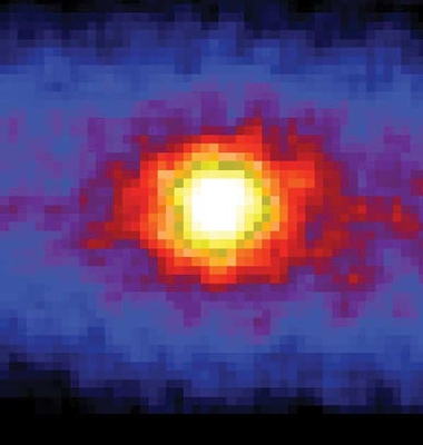
The Sun at night. Solar neutrinos as detected by Super-Kamioknade looking through the Earth. I think this is the astronomical equivalent of checking if the fridge light does go off when you close the door. Credit: Marcus Chown & Super-Kamiokande.
The mystery of the missing neutrinos
Detecting solar neutrinos was a big success, but there was a problem. There were only a fraction of the predicted number. This became known as the solar neutrino problem. There were two possibilities, either solar physicists had got their models wrong, or particle physicists were missing a part of the Standard Model.
The solar models were recalculated and tweaked, with much work done by John Bahcall and collaborators. More sophisticated calculations were performed, even folding in new data from helioseismology, the study of waves in the Sun, but the difference could not be resolved.
However, there was an idea in particle physics by Bruno Pontecorvo and Vladimir Gribov: that neutrinos could change flavour, a phenomena known as neutrino oscillations. This was actually first suggested before the first Homestake results were announced, perhaps it deserved further attention?
The first evidence in favour of neutrino oscillations comes from Super-Kamiokande, the successor to the original Kamiokande. This evidence came from looking at neutrinos produced by cosmic rays. Cosmic rays are highly energetic particles that come from space. As they slam into the atmosphere, and collide with molecules in the air, they produce a shower of particles. These include muons and muon-neutrinos. Super-Kamiokande could detect muon-neutrinos from cosmic rays. Cosmic rays come from all directions, so Super-Kamiokande should see muon-neutrinos from all directions too. Just like we can see the solar neutrinos through the Earth, we should see muon-neutrinos both from above and below. However, more were detected from above than below.
Something must happen to muon-neutrinos during their journey through the Earth. Super-Kamiokande could detect them as electron-neutrinos or muon-neutrinos, but is not sensitive to tau-neutrinos. This is evidence that muon-neutrinos were changing flavour to tau-neutrinos.
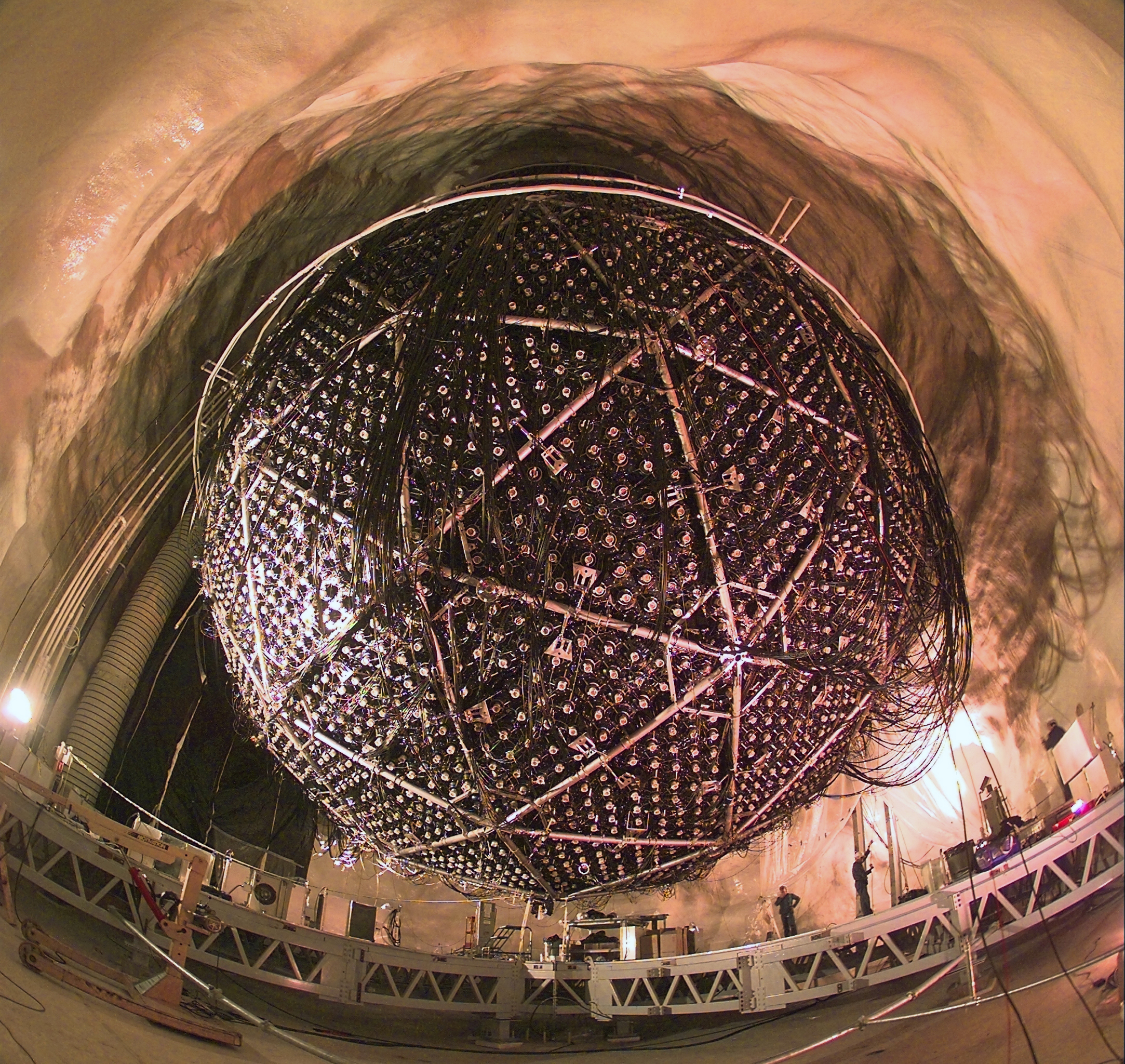
The Sudbury Neutrino Observatory detector, a 12-metre sphere containing 1000 tonnes of heavy water which is two kilometres underground. Credit: SNOLAB.
The solar neutrino problem was finally solved in 2001 through measurements of the Sudbury Neutrino Observatory (SNO). SNO is another Cherenkov detector like (Super-)Kamiokande, but it used heavy water instead of regular water. (High-purity heavy water is extremely expensive, it would have cost hundreds of millions of dollars for SNO to buy the 1000 tonnes it used, so it managed to secure it on loan from Atomic Energy of Canada Limited). Using heavy water meant that SNO was sensitive to all flavours of neutrinos. Like previous experiments, SNO found that there were not as many electron-neutrinos from the Sun as expected. However, there were also muon-neutrinos and tau-neutrinos, and when these were added, the total worked out!
The solar astrophysicists had been right all along, what was missing was that neutrinos oscillate between flavours. Studying the Sun had led to a discovery about some of the smallest particles in Nature.
Neutrino oscillations
Experiments have shown that neutrino oscillations occur, but how does this work? We need to delve into quantum mechanics.
The theory of neutrino oscillations say that each of the neutrino flavours corresponds to a different combination of neutrino mass states. This is weird, it means that if you were to somehow weight an electron-, muon- or tau-neutrino, you would get one of three values, but which one is random (although on average, each flavour would have a particular mass). By rearranging the mass states into a different combination you can get a different neutrino flavour. While neutrinos are created as a particular flavour, when they travel, the mass states rearrange relative to each other, so when they arrive at their destination, they could have changed flavour (or even changed flavour and then changed back again).
To get a more detailed idea of what’s going on, we’ll imagine the simpler case of there being only two neutrino flavours (and two neutrino mass states). We can picture a neutrino as a clock face with an hour hand and a minute hand. These represent the two mass states. Which neutrino flavour we have depends upon their relative positions. If they point in the same direction, we have one flavour (let’s say mint) and if they point in opposite directions, we have the other (orange). We’ll create a mint neutrino at 12 noon and watch it evolve. The hands more at different speeds, so at ~12:30 pm, they are pointing opposite ways, and our neutrino has oscillated into an orange neutrino. At ~1:05 pm, the hands are aligned again, and we’re back to mint. Which neutrino you have depends when you look. At 3:30 am, you’ll have a roughly even chance of finding either flavour and at 6:01 pm, you’ll be almost certain to have orange neutrino, but there’s still a tiny chance of finding an mint one. As time goes on, the neutrino oscillates back and forth.
With three neutrinos flavours, things are more complicated, but the idea is similar. You can imagine throwing in a second hand and making different flavours based upon the relative positions of all three hands.
We can now explain why Super-Kamiokande saw different numbers of muon-neutrinos from different sides of the Earth. Those coming from above only travel a short distance, there’s little time between when they were created and when they are detected, so there’s not much chance they’ll change flavour. Those coming through the Earth have had enough time to switch flavour.
A similar thing happens as neutrinos travel from the core of the Sun out to the surface. (There’s some interesting extra physics that happens here too. A side effect of there being so much matter at the centre of the Sun, the combination of mass states that makes up the different flavours is different than at the outside. This means that even without the hands on the clock going round, we can get a change in flavour).
Neutrino oscillations happen because neutrino mass states are not the same as the flavour states. This requires that neutrinos have mass. In the Standard Model, neutrinos are massless, so the Standard Model had to be extended.
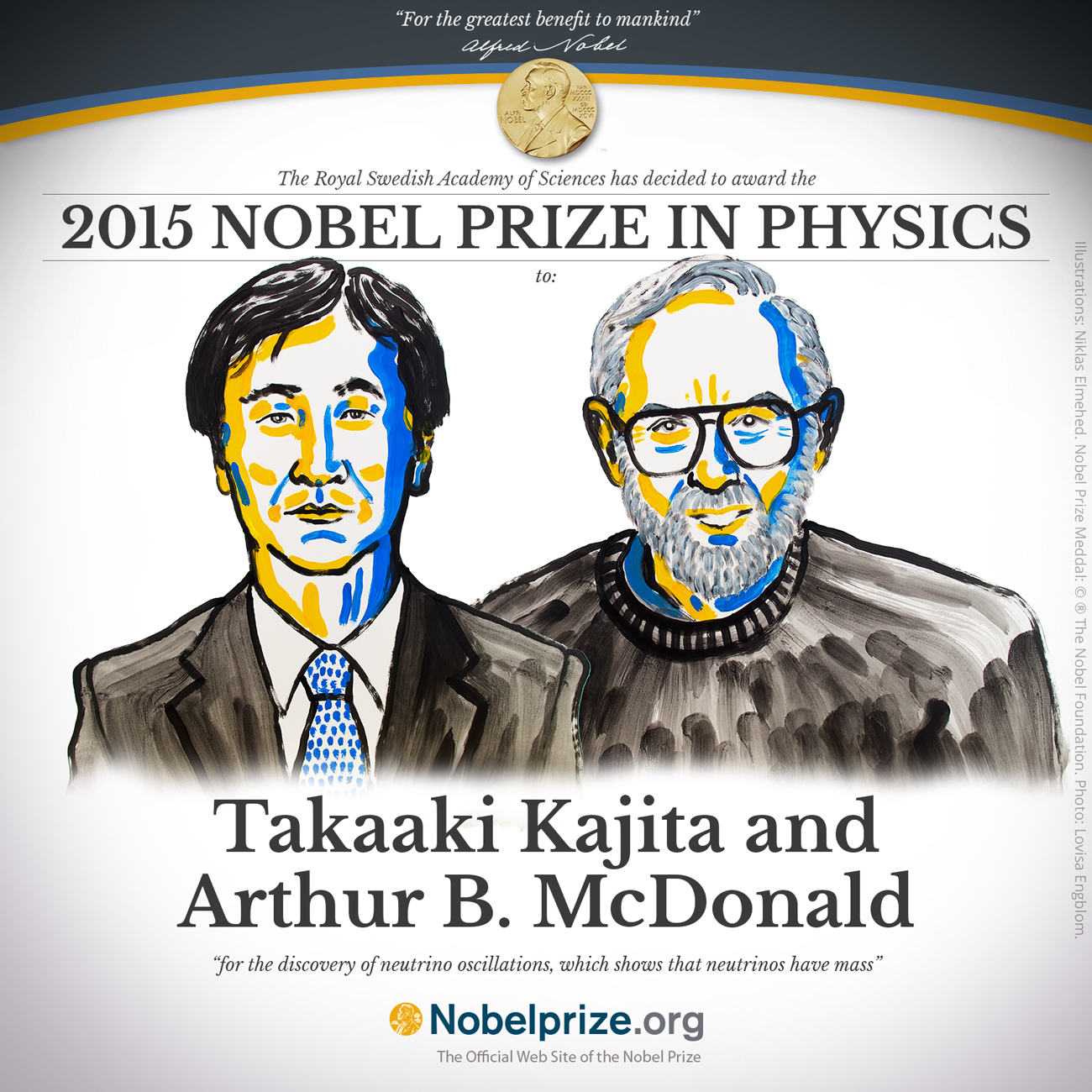
2015 Physics Nobel laureates, Takaaki Kajita and Arthur B. McDonald. Credit: Nobel Foundation.
Happy ending
For confirming that neutrinos have mass, Takaaki Kajita of Super-Kamiokande and Arthur McDonald of SNO won this year’s Nobel Prize. It is amazing how much physics has been discovered from trying to answer as simple a question as how does the Sun shine?
Even though neutrinos are shy, they are really interesting characters when you get to know them.
Now that the mystery of the missing neutrinos is solved, what is next? Takaaki Kajita is now involved in another project in the Kamioka Mine, the construction of KAGRA, a gravitational-wave detector.
The control room of KAGRA, the gravitational-wave detector in the Hida Mountains, Japan. I visited June 2015. Could a third Nobel come out of the Kamioka Mine?
Athene Donald, Professor of Experimental Physics and soon-to-be Master of my old college, Churchill, recently blogged about how athletics resembles academia. She argued that both are hard careers: they require many years of training, and even then success is not guaranteed—not everyone will reach the top to become an Olympian or a Professor—there is a big element of luck too—a career can stall because of an injury or because of time invested in a study that eventually yields null results, and, conversely, a single big championship win or serendipitous discovery can land a comfortable position. These factors can make these career paths unappealing, but still most people who enter them do so because they love the area, and have a real talent for the field.
As The Breakfast Club taught us, being into physics or sports can have similar pressures.
I find this analogy extremely appealing. There are many parallels. Both sports and academic careers are meritocratic and competitive. Most who enter them will not become rich—those who do, usually manage it by making use of their profile, either through product endorsement or through writing a book, say Stephen Hawking, or Michael Jordan (although he was still extremely well paid). Both fields have undisputed heavy-weights like Einstein or Muhammad Ali, and media superstars like Neil deGrasse Tyson or Anna Kournikova; both have inspirational figures who have overcome adversity, be they Jesse Owens or Emmy Noether, and idols whose personal lives you probably shouldn’t emulate, say Tiger Woods or Richard Feynman. However, I think the similarity can stretch beyond career paths.
Athene says that although she doesn’t participate in athletics, she does enjoy watching the sport. I’m sure many can empathise with that position. I think that this is similarly the case for research: many enjoy finding out about new discoveries or ideas, even though they don’t want to invest the time studying themselves. There are many excellent books and documentaries, many excellent communicators of research. (I shall be helping out at this year’s British Science Festival, which I’m sure will be packed with people keen to find out about current research.) However, there is undoubtedly more that could be done, both in terms of growing the market and improving the quality—reporting of science is notoriously bad. If you were to go into any pub in the country, I’d expect you’d be able to find someone to have an in-depth conversation with about how best to manage the national football team, despite them not being a professional footballer. Why not someone with similar opinions about research council funding? Can we make research as popular as sport?
Increasing engagement with and awareness of research is a popular subject, most research grants with have some mention of wider impact; however, I don’t think that this is the only goal. According to UK government research, many young students do enjoy science, they just don’t feel it is for them. The problem is that people think that science is too difficult. Given my previous ramblings, that’s perhaps understandable. However, that was for academic research; science is far broader than that! There are many careers outside the lab, and understanding science is useful even if that’s not your job, for example when discussing subjects like global warming or vaccination that affect us all. Coming back to our sports analogy, the situation is like children not wanting to play football because they won’t be a professional. It’s true that most people aren’t good enough to play for England (potentially including members of the current squad, depending upon who you ask in that pub), but that doesn’t mean you can’t enjoy a kick around, perhaps play for a local team at weekend, or even coach others. Playing sports regular keeps you physically fit, which is a good thing™; taking an interest in science (or language or literature or etceteras) keeps you mentally fit, also a good thing™.
Chocolate is also a good thing™. However, neither Nobel Prizes nor Olympic Medals are made of chocolate, something I’m not sure that everyone appreciates. I’d make the gold Olympic models out of milk chocolate, silver out of white and bronze out of dark. The Nobel Prize for Medicine should contain nuts as an incentive to cure allergies; the Prize for Economics should be mint(ed) chocolate, the Peace Prize Swiss chocolate, the Chemistry Prize should contain popping candy, and the Physics Prize should be orange chocolate (that’s my favourite).
How to encourage more people to engage in science is a complicated problem. There’s no single solution, but it is something to work on. I would definitely prefer to live in a science-literate society. Stressing applications of science beyond pure research might be one avenue. I would also like to emphasis that it’s OK to find science (and maths) hard. Problem solving is difficult, like long-distance running, but if you practise, it does get easier. I can only vouch for one side of that simile from personal experience, but since I’m a theoretician, I’m happy enough to state that without direct experimental confirmation. I guess that means I should take my own advice and participate more myself: spend a little more time being physically active? Motivating myself is also a difficult problem.


 ). The lower panel shows how we removed the glitch: the grey line shows


 is the component of the spin aligned with the orbital angular momentum. The two-dimensional shows the 90% probability contour, which follows a line of constant chirp mass. The one-dimensional plot shows individual masses; the dotted lines mark 90% bounds away from equal mass. Figure 4 of the
  .
.
 inferred from GW170817. The lines mark 68% and 95% intervals. The coloured bands are measurements from the cosmic microwave background (
 (assuming a uniform of neutron star masses between one and two solar masses). This is surprisingly close to what the Collaboration expected back in
  and
and  , with a realistic rate of
  . This means that we are on track to see many more binary neutron stars—perhaps one a week at design sensitivity!


 and
and  ), and the black hole they merge to form (
 ), they are all quite similar
 ,
,  ,
,  ;
; ,
,  ,
,  ;
; ,
,  ,
,  .
. , a particular combination of the two component spins that influences how they inspiral together, and the spin of the final black hole
 ,
,  ;
; ,
,  ;
; ,
, 


 direction. (a) and (b) are the plus and cross tensor polarizations of general relativity. (c) and (d) are the scalar breathing and longitudinal modes, and (e) and (f) are the vector
  and
and  polarizations. The tensor polarizations (in red) are transverse, the vector and longitudinal scalar mode (in green) are longitudinal. The scalar breathing mode (in blue) is an isotropic expansion and contraction, so its a bit of a mix of transverse and longitudinal. Figure 10 from (the excellent)
  , and their antiparticle equivalents (antineutrinos) are denoted by
  . We’ll not worry about the difference between the two. Neutrinos are rather shy. They are quite happy doing their own thing, and don’t interact much with other particles. They don’t have an electric charge (they are neutral), so they don’t play with the electromagnetic force (and photons), they also don’t do anything with the strong force (and gluons). They only get involved with the weak force (W and Z bosons). As you might expect from the name, the weak force doesn’t do much (it only operates over short distances), so spotting a neutrino is a rare occurrence.
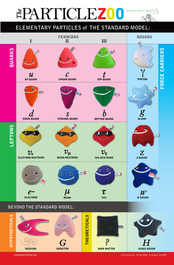
 , the muon-neutrino
  (
( is the Greek letter mu) and the tau-neutrino
  (
( is the Greek letter tau).
 ), which are the nuclei of hydrogen, are converted to Helium nuclei after a sequence of steps. Electron neutrinos