An introduction to LIGO–Virgo data analysis

February 9, 2020January 25, 2021 / CPLB / Leave a comment

LIGO and Virgo make their data open for anyone to try analysing [bonus note]. If you’re a student looking for a project, a teacher planning a class activity, or a scientist working on a paper, this data is waiting for you to use. Understanding how to analyse the data can be tricky. In this post, I’ll share some of the resources made by LIGO and Virgo to help introduce gravitational-wave analysis. These papers together should give you a good grounding in how to get started working with gravitational-wave data.

If you’d like a more in-depth understanding, I’d recommend visiting your local library for Michele Maggiore’s Gravitational Waves: Volume 1.

The Data Analysis Guide

Title: A guide to LIGO-Virgo detector noise and extraction of transient gravitational-wave signals
arXiv: 1908.11170 [gr-qc]
Journal: Classical & Quantum Gravity; 37(5):055002(54); 2020
Tutorial notebook: GitHub; Google Colab; Binder
Code repository: Data Guide
LIGO science summary: A guide to LIGO-Virgo detector noise and extraction of transient gravitational-wave signals

It took many decades to develop the technology necessary to build gravitational-wave detectors. Similarly, gravitational-wave data analysis has developed over many decades—I’d say LIGO analysis was really kicked off in the early 1990s by Kipp Thorne’s group. There are now hundreds of papers on various aspects of gravitational-wave analysis. If you are new to the area, where should you start? Don’t panic! For the binary sources discovered so far, this Data Analysis Guide has you covered.

More details: The Data Analysis Guide

The GWOSC Paper

Title: Open data from the first and second observing runs of Advanced LIGO and Advanced Virgo
arXiv: 1912.11716 [gr-qc]
Journal: SoftwareX; 13:100658(20); 2021
Website: Gravitational Wave Open Science Center
LIGO science summary: Open data from the first and second observing runs of Advanced LIGO and Advanced Virgo

Data from the LIGO and Virgo detectors is released by the Gravitational Wave Open Science Center (GWOSC, pronounced, unfortunately, as it is spelt). If you want to try analysing our delicious data yourself, either searching for signals or studying the signals we have found, GWOSC is the place to start. This paper outlines how these data are produced, going from our laser interferometers to your hard-drive. The paper specifically looks at the data released for our first and second observing runs (O1 and O2), however, GWOSC also host data from the initial detectors’ fifth science run (S5) and sixth science run (S6), and will be updated with new data in the future.

If you do use data from GWOSC, please remember to say thank you.

More details: The GWOSC Paper

001100 010010 011110 100001 101101 110011

I thought I saw a 2! Credit: Fox

The Data Analysis Guide

Synopsis: Data Analysis Guide
Read this if: You want an introduction to signal analysis
Favourite part: This is a great resource for new students [bonus note]

Gravitational-wave detectors measure ripples in spacetime. They record a simple time series of the stretching and squeezing of space as a gravitational wave passes. Well, they measure that, plus a whole lot of noise. Most of the time it is just noise. How do we go from this time series to discoveries about the Universe’s black holes and neutron stars? This paper gives the outline, it covers (in order)

An introduction to observations at the time of writing
The basics of LIGO and Virgo data—what it is the we analyse
The basics of detector noise—how we describe sources of noise in our data
Fourier analysis—how we go from time series to looking at the data in the as a function of frequency, which is the most natural way to analyse that data.
Time–frequency analysis and stationarity—how we check the stability of data from our detectors
Detector calibration and data quality—how we make sure we have good quality data
The noise model and likelihood—how we use our understanding of the noise, under the assumption of it being stationary, to work out the likelihood of different signals being in the data
Signal detection—how we identify times in the data which have a transient signal present
Inferring waveform and physical parameters—how we estimate the parameters of the source of a gravitational wave
Residuals around GW150914—a consistency check that we have understood the noise surrounding our first detection

The paper works through things thoroughly, and I would encourage you to work though it if you are interested.

I won’t summarise everything here, I want to focus the (roughly undergraduate-level) foundations of how we do our analysis in the frequency domain. My discussion of the GWOSC Paper goes into more detail on the basics of LIGO and Virgo data, and some details on calibration and data quality. I’ll leave talking about residuals to this bonus note, as it involves a long tangent and me needing to lie down for a while.

Fourier analysis

The signal our detectors measure is a time series $d(t)$ . This is may just contain noise, $d(t) = n(t)$ , or it may also contain a signal, $d(t) = n(t) + h(t)$ .

There are many sources of noise for our detectors. The different sources can affect different frequencies. If we assume that the noise is stationary, so that it’s properties don’t change with time, we can simply describe the properties of the noise with the power spectral density $S_n(f)$ . On average we expect the noise at a given frequency to be zero, but with it fluctuating up and down with a variance given by the power spectral density. We typically approximate the noise as Gaussian, such that

$n(f) \sim \mathcal{N}(0; S_n(f)/2)$ ,

where we use $\mathcal{N}(\mu; \sigma^2)$ to represent a normal distribution with mean $\mu$ and standard deviation $\sigma$ . The approximations of stationary and Gaussian noise are good most of the time. The noise does vary over time, but is usually effectively stationary over the durations we look at for a signal. The noise is also mostly Gaussian except for glitches. These are taken into account when we search for signals, but we’ll ignore them for now. The statistical description of the noise in terms of the power spectral density allows us to understand our data, but this understanding comes as a function of frequency: we must transform of time domain data to frequency domain data.

The go from $d(t)$ to $d(f)$ we can use a Fourier transform. Fourier transforms are a way of converting a function of one variable into a function of a reciprocal variable—in the case of time you convert to frequency. Fourier transforms encode all the information of the original function, so it is possible to convert back and forth as you like. Really, a Fourier transform is just another way of looking at the same function.

The Fourier transform is defined as

$d(f) = \mathcal{F}_f\left\{d(t)\right\} = \int_{-\infty}^{\infty} d(t) \exp(-2\pi i f t) \,\mathrm{d}t$ .

Now, from this you might notice a problem when it comes to real data analysis, namely that the integral is defined over an infinite amount of time. We don’t have that much data. Instead, we only have a short period.

We could recast the integral above over a shorter time if instead of taking the Fourier transform of $d(t)$ , we take the Fourier transform of $d(t) \times w(t)$ where $w(t)$ is some window function which goes to zero outside of the time interval we are looking at. What we end up with is a convolution of the function we want with the Fourier transform of the window function,

$\mathcal{F}_f\left\{d(t)w(t)\right\} = d(f) \ast w(f)$ .

It is important to pick a window function which minimises the distortion to the signal that we want. If we just take a tophat (also known as a boxcar or rectangular, possibly on account of its infamous criminal background) function which is abruptly cuts off the data at the ends of the time interval, we find that $w(f)$ is a sinc function. This is not a good thing, as it leads to all sorts of unwanted correlations between different frequencies, commonly known as spectral leakage. A much better choice is a function which smoothly tapers to zero at the edges. Using a tapering window, we lose a little data at the edges (we need to be careful choosing the length of the data analysed), but we can avoid the significant nastiness of spectral leakage. A tapering window function should always be used. Then or finite-time Fourier transform is then a good approximation to the exact $d(f)$ .

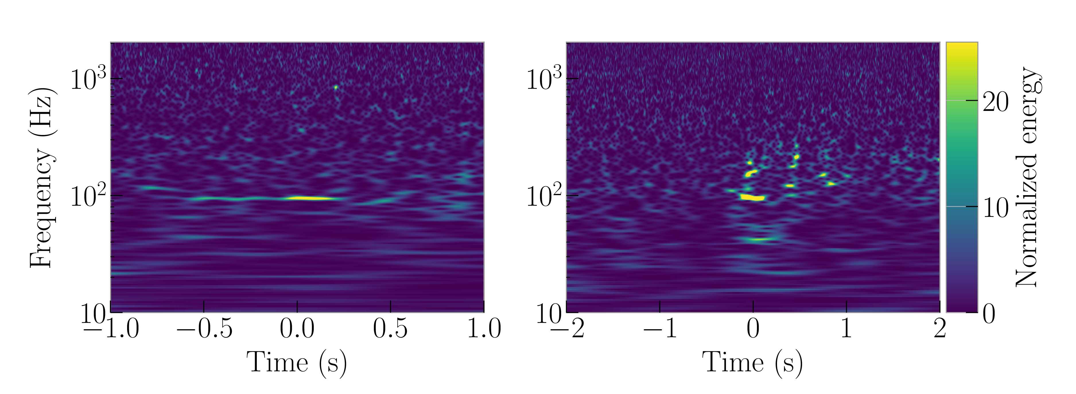
Data processing to reveal GW150914. The top panel shows raw Hanford data. The second panel shows a window function being applied. The third panel shows the data after being whitened. This cleans up the data, making it easier to pick out the signal from all the low frequency noise. The bottom panel shows the whitened data after a bandpass filter is applied to pick out the signal. We don’t use the bandpass filter in our analysis (it is just for illustration), but the other steps reflect how we treat our data. Figure 2 of the Data Analysis Guide.

Now we have our data in the frequency domain, it is simple enough to compare the data to the expected noise a t a given frequency. If we measure something loud at a frequency with lots of noise we should be less surprised than if we measure something loud at a frequency which is usually quiet. This is kind of like how somewhat shouting is less startling at a rock concert than in a library. The appropriate way to weight is to divide by the square root of power spectral density $d_\mathrm{w}(f) \propto d(f)/[S_n(f)]^{1/2}$ . This is known as whitening. Whitened data should have equal amplitude fluctuations at all frequencies, allowing for easy comparisons.

Now we understand the statistical properties of noise we can do some analysis! We can start by testing our assumption that the data are stationary and Gaussian by checking that that after whitening we get the expected distribution. We can also define the likelihood of obtaining the data $d(t)$ given a model of a gravitational-wave signal $h(t)$ , as the properties of the noise mean that $d(f) - h(f) \sim \mathcal{N}(0; S_n(f)/2)$ . Combining the likelihood for each individual frequency gives the overall likelihood

$\displaystyle p(d|h) \propto \exp\left[-\int_{-\infty}^{\infty} \frac{|d(f) - h(f)|^2}{S_n(f)} \mathrm{d}f \right]$ .

This likelihood is at the heart of parameter estimation, as we can work out the probability of there being a signal with a given set of parameters. The Data Analysis Guide goes through many different analyses (including parameter estimation) and demonstrates how to check that noise is nice and Gaussian.

Distribution of residuals for 4 seconds of data around GW150914 after subtracting the maximum likelihood waveform. The residuals are the whitened Fourier amplitudes, and they should be consistent with a unit Gaussian. The residuals follow the expected distribution and show no sign of non-Gaussianity. Figure 14 of the Data Analysis Guide.

Homework

The Data Analysis Guide contains much more material on gravitational-wave data analysis. If you wanted to delve further, there many excellent papers cited. Favourites of mine include Finn (1992); Finn & Chernoff (1993); Cutler & Flanagan (1994); Flanagan & Hughes (1998); Allen (2005), and Allen et al. (2012). I would also recommend the tutorials available from GWOSC and the lectures from the Open Data Workshops.

The GWOSC Paper

Synopsis: GWOSC Paper
Read this if: You want to analyse our gravitational wave data
Favourite part: All the cool projects done with this data

You’re now up-to-speed with some ideas of how to analyse gravitational-wave data, you’ve made yourself a fresh cup of really hot tea, you’re ready to get to work! All you need are the data—this paper explains where this comes from.

Data production

The first step in getting gravitational-wave data is the easy one. You need to design a detector, convince science agencies to invest something like half a billion dollars in building one, then spend 40 years carefully researching the necessary technology and putting it all together as part of an international collaboration of hundreds of scientists, engineers and technicians, before painstakingly commissioning the instrument and operating it. For your convenience, we have done this step for you, but do feel free to try it yourself at home.

Gravitational-wave detectors like Advanced LIGO are built around an interferometer: they have two arms at right angles to each other, and we bounce lasers up and down them to measure their length. A passing gravitational wave will change the relative length of one arm relative to the other. This changes the time taken to travel along one arm compared to the other. Hence, when the two bits of light reach the output of the interferometer, they’ll have a different phase:where normally one light wave would have a peak, it’ll have a trough. This change in phase will change how light from the two arms combine together. When no gravitational wave is present, the light interferes destructively, almost cancelling out so that the output is dark. We measure the brightness of light at the output which tells us about how the length of the arms changes.

We want our detector in measure the gravitational-wave strain. That is the fractional change in length of the arms,

$\displaystyle h(t) = \frac{\Delta L(t)}{L}$ ,

where $\Delta L = L_x - L_y$ is the relative difference in the length of the two arms, and $L$ is the usually arm length. Since we love jargon in LIGO & Virgo, we’ll often refer to the strain as HOFT (as you would read $h(t)$ as h of t; it took me years to realise this) or DARM (differential arm measurement).

The actual output of the detector is the voltage from a photodiode measuring the intensity of the light. It is necessary to make careful calibration of the detectors. In theory this is simple: we change the position of the mirrors at the end of the arms and see how the output changes. In practise, it is very difficult. The GW150914 Calibration Paper goes into details for O1, more up-to-date descriptions are given in Cahillane et al. (2017) for LIGO and Acernese et al. (2018) for Virgo. The calibration of the detectors can drift over time, improving the calibration is one of the things we do between originally taking the data and releasing the final data.

The data are only celebrated between 10 Hz and 5 kHz, so don’t trust the data outside of that frequency range.

The next stage of our data’s journey is going through detector characterisation and data quality checks. In addition to measuring gravitational-wave strain, we record many other data channels: about 200,000 per detector. These measure all sorts of things, from the internal state of the instrument, to monitoring the physical environment around the detectors. These auxiliary channels are used to check the data quality. In some cases, an auxiliary channel will record a source of noise, like scattered light or the mains power frequency, allowing us to clean up our strain data by subtracting out this noise. In other cases, an auxiliary channel can act as a witness to a glitch in our detector, identifying when it is misbehaving so that we know not to trust that part of the data. The GW150914 Detector Characterisation Paper goes into details of how we check potential detections. In doing data quality checks we are careful to only use the auxiliary channels which record something which would be independent of a passing gravitational wave.

We have 4 flags for data quality:

DATA: All clear. Certified fresh. Eat as much as you like.
CAT1: A critical problem with the instrument. Data from these times are likely to be a dumpster fire of noise. We do not use them in our analyses, and they are currently excluded from our public releases. About 1.7% of Hanford data and 1.0% of time from Livingston was flagged with CAT1 in O1. In O2, we got this done to 0.001% for Hanford, 0.003% for Livingston and 0.05% for Virgo.
CAT2: Some activity in an auxiliary channel (possibly the electric boogaloo monitor) which has a well understood correlation with the measured strain channel. You would therefore expect to find some form of glitchiness in the data.
CAT3: There is some correlation in an auxiliary channel and the strain channel which is not understood. We’re not currently using this flag, but it’s kept as an option.

It’s important to verify the data quality before starting your analysis. You don’t want to get excited to discover a completely new form of gravitational wave only to realise that it’s actually some noise from nearby logging. Remember, if a tree falls in the forest and no-one is around, LIGO will still know.

To test our systems, we also occasionally perform a signal injection: we move the mirrors to simulate a signal. This is useful for calibration and for testing analysis algorithms. We don’t perform injections very often (they get in the way of looking for real signals), but these times are flagged. Just as for data quality flags, it is important to check for injections before analysing a stretch of data.

Once passing through all these checks, the data is ready to analyse!

Excited Data. Credit: Paramount

Accessing the data

After our data have been lovingly prepared, they are served up in two data formats:

Hierarchical Data Format HDF, which is a popular data storage format, as it is easily allows for metadata and multiple data sets (like the important data quality flags) to be packaged together.
Gravitational Wave Frame GWF, which is the standard format we use internally. Veteran gravitational-wave scientists often get a far-way haunted look when you bring up how the specifications for this file format were decided. It’s best not to mention unless you are also buying them a stiff drink.

In these files, you will find $h(t)$ sampled at either 4096 Hz or 16384 Hz (either are available). Pick the sampling rate you need depending upon the frequency range you are interested in: the 4096 Hz data are good for upto 1.7 kHz, while the 16384 Hz are good to the limit of the calibration range at 5 kHz.

Files can be downloaded from the GWOSC website. If you want to download a large amount, it is recommended to use the CernVM-FS distributed file system.

To check when the gravitational-wave detectors were observing, you can use the Timeline search.

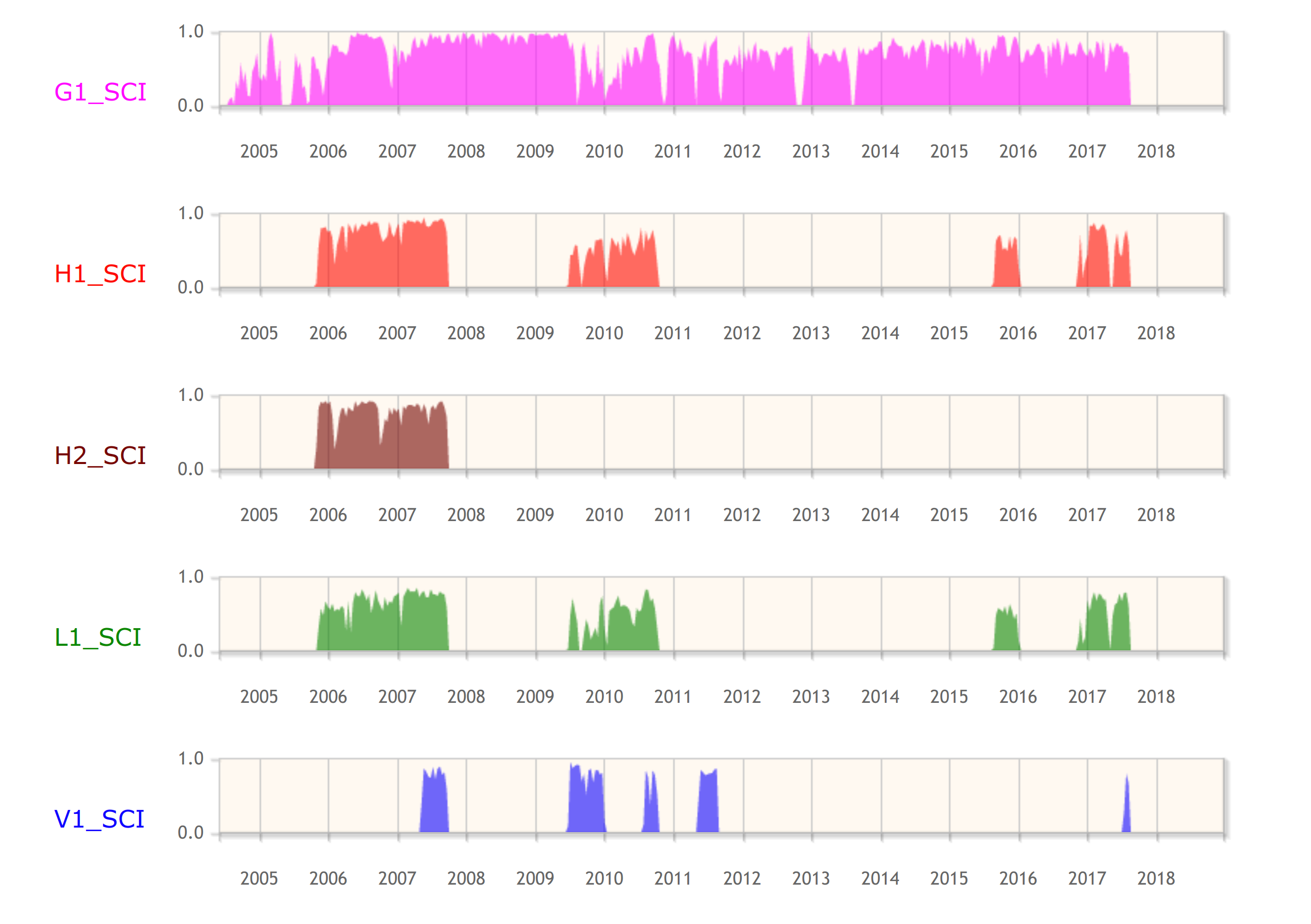
Screenshot of the GWOSC Timeline showing observing from the fifth science run (S5) on the initial detector era through to the second observing run (O2) of the advanced detector era. Bars show observing of GEO 600 (G1), Hanford (H1 and H2), Livingston (L1) and Virgo (V1). Hanford initial had two detectors housed within its site, the plan in the advanced detector era is to install the equipment as LIGO India instead.

Try this at home

Having gone through all these details, you should now know what are data is, over what ranges it can be analyzed, and how to get access to it. Your cup of tea has also probably gone cold. Why not make yourself a new one, and have a couple of biscuits as reward too. You deserve it!

To help you on your way in starting analysing the data, GWOSC has a set of tutorials (and don’t forget the Data Analysis Guide), and a collection of open source software. Have fun, and remember, it’s never aliens.

Bonus notes

Release schedule

The current policy is that data are released:

In a chunk surrounding an event at time of publication of that event. This enables the new detection to be analysed by anyone. We typically release about an hour of data around an event.
18 months after the end of the run. This time gives us chance to properly calibrate the data, check the data quality, and then run the analyses we are committed to. A lot of work goes into producing gravitational wave data!

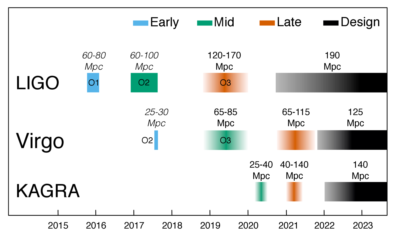
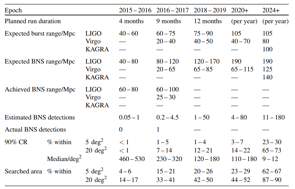
Start marking your calendars now for the release of O3 data.

Summer studenting

In summer 2019, while we were finishing up on the Data Analysis Guide, I gave it to one of my summer students Andrew Kim as an introduction. Andrew was working on gravitational-wave data analysis, so I hoped that he’d find it useful. He ended up working through the draft notebook made to accompany the paper and making a number of useful suggestions! He ended up as an author on the paper because of these contributions, which was nice.

The conspiracy of residuals

The Data Analysis Guide is an extremely useful paper. It explains many details of gravitational-wave analysis. The detections made by LIGO and Virgo over the last few years has increased the interest in analysing gravitational waves, making it the perfect time to write such an article. However, that’s not really what motivated us to write it.

In 2017, a paper appeared on the arXiv making claims of suspicious correlations in our LIGO data around GW150914. Could this call into question the very nature of our detection? No. The paper has two serious flaws.

The first argument in the paper was that there were suspicious phase correlations in the data. This is because the authors didn’t window their data before Fourier transforming.
The second argument was the residuals presented in Figure 1 of the GW150914 Discovery Paper contain a correlation. This is true, but these residuals aren’t actually the results of how we analyse the data. The point of Figure 1 was to that you don’t need our fancy analysis to see the signal—you can spot it by eye. Unfortunately, doing things by eye isn’t perfect, and this imperfection was picked up on.

The first flaw is a rookie mistake—pretty much everyone does it at some point. I did it starting out as a first-year PhD student, and I’ve run into it with all the undergraduates I’ve worked with writing their own analyses. The authors of this paper are rookies in gravitational-wave analysis, so they shouldn’t be judged too harshly for falling into this trap, and it is something so simple I can’t blame the referee of the paper for not thinking to ask. Any physics undergraduate who has met Fourier transforms (the second year of my degree) should grasp the mistake—it’s not something esoteric you need to be an expert in quantum gravity to understand.

The second flaw is something which could have been easily avoided if we had been more careful in the GW150914 Discovery Paper. We could have easily aligned the waveforms properly, or more clearly explained that the treatment used for Figure 1 is not what we actually do. However, we did write many other papers explaining what we did do, so we were hardly being secretive. While Figure 1 was not perfect, it was not wrong—it might not be what you might hope for, but it is described correctly in the text, and none of the LIGO–Virgo results depend on the figure in any way.

Estimated waveforms from different models

Recovered gravitational waveforms from our analysis of GW150914. The grey line shows the data whitened by the noise spectrum. The dark band shows our estimate for the waveform without assuming a particular source. The light bands show results if we assume it is a binary black hole (BBH) as predicted by general relativity. This plot more accurately represents how we analyse gravitational-wave data. Figure 6 of the GW150914 Parameter Estimation Paper.

Both mistakes are easy to fix. They are at the level of “Oops, that’s embarrassing! Give me 10 minutes. OK, that looks better”. Unfortunately, that didn’t happen.

The paper regrettably got picked up by science blogs, and caused much of a flutter. There were demands that LIGO and Virgo publically explain ourselves. This was difficult—the Collaboration is set up to do careful science, not handle a PR disaster. One of the problems was that we didn’t want to be seen to policing the use of our data. We can’t check that every paper ever using our data does everything perfectly. We don’t have time, and that probably wouldn’t encourage people to use our data if they knew any mistake would be pulled up by this 1000 person collaboration. A second problem was that getting anything approved as an official Collaboration document takes ages—getting consensus amongst so many people isn’t always easy. What would you do—would you want to be the faceless Collaboration persecuting the helpless, plucky scientists trying to check results?

There were private communications between people in the Collaboration and the authors. It took us a while to isolate the sources of the problems. In the meantime, pressure was mounting for an official™ response. It’s hard to justify why your analysis is correct by gesturing to a stack of a dozen papers—people don’t have time to dig through all that (I actually sent links to 16 papers to a science journalist who contacted me back in July 2017). Our silence may have been perceived as arrogance or guilt.

It was decided that we would put out an unofficial response. Ian Harry had been communicating with the authors, and wrote up his notes which Sean Carroll kindly shared on his blog. Unfortunately, this didn’t really make anyone too happy. The authors of the paper weren’t happy that something was shared via such an informal medium; the post is too technical for the general public to appreciate, and there was a minor typo in the accompanying code which (since fixed) was seized upon. It became necessary to write a formal paper.

Oh, won't somebody please think of the children?

Peer review will save the children! Credit: Fox

We did continue to try to explain the errors to the authors. I have colleagues who spent many hours in a room in Copenhagen trying to explain the mistakes. However, little progress was made, and it was not a fun time™. I can imagine at this point that the authors of the paper were sufficiently angry not to want to listen, which is a shame.

Now that the Data Analysis Guide is published, everyone will be satisfied, right? A refereed journal article should quash all fears, surely? Sadly, I doubt this will be the case. I expect these doubts will keep circulating for years. After all, there are those who still think vaccines cause autism. Fortunately, not believing in gravitational waves won’t kill any children. If anyone asks though, you can tell them that any doubts on LIGO’s analysis have been quashed, and that vaccines cause adults!

For a good account of the back and forth, Natalie Wolchover wrote a nice article in Quanta, and for a more acerbic view, try Mark Hannam’s blog.

Classifying the unknown: Discovering novel gravitational-wave detector glitches using similarity learning

January 12, 2020August 1, 2020 / CPLB / Leave a comment

Gravity Spy is an awesome project that combines citizen science and machine learning to classify glitches in LIGO and Virgo data. Glitches are short bursts of noise in our detectors which make analysing our data more difficult. Some glitches have known causes, others are more mysterious. Classifying glitches into different types helps us better understand their properties, and in some cases track down their causes and eliminate them! In this paper, led by Scotty Coughlin, we demonstrated the effectiveness of a new tool which are citizen scientists can use to identify new glitch classes.

The Gravity Spy project

Gravitational-wave detectors are complicated machines. It takes a lot of engineering to achieve the required accuracy needed to observe gravitational waves. Most of the time, our detectors perform well. The background noise in our detectors is easy to understand and model. However, our detectors are also subject to glitches, unusual (sometimes extremely loud and complicated) noise that doesn’t fit the usual properties of noise. Glitches are short, they only appear in a small fraction of the total data, but they are common. This makes detection and analysis of gravitational-wave signals more difficult. Detection is tricky because you need to be careful to distinguish glitches from signals (and possibly glitches and signals together), and understanding the signal is complicated as we may need to model a signal and a glitch together [bonus note]. Understanding glitches is essential if gravitational-wave astronomy is to be a success.

To understand glitches, we need to be able to classify them. We can search for glitches by looking for loud pops, whooshes and splats in our data. The task is then to spot similarities between them. Once we have a set of glitches of the same type, we can examine the state of the instruments at these times. In the best cases, we can identify the cause, and then work to improve the detectors so that this no longer happens. Other times, we might be able to find the source, but we can find one of the monitors in our detectors which acts a witness to the glitch. Then we know that if something appears in that monitor, we expect a glitch of a particular form. This might mean that we throw away that bit of data, or perhaps we can use the witness data to subtract out the glitch. Since glitches are so common, classifying them is a huge amount of work. It is too much for our detector characterisation experts to do by hand.

There are two cunning options for classifying large numbers of glitches

Get a computer to do it. The difficulty is teaching a computer to identify the different classes. Machine-learning algorithms can do this, if they are properly trained. Training can require a large training set, and careful validation, so the process is still labour intensive.
Get lots of people to help. The difficulty here is getting non-experts up-to-speed on what to look for, and then checking that they are doing a good job. Crowdsourcing classifications is something citizen scientists can do, but we will need a large number of dedicated volunteers to tackle the full set of data.

The idea behind Gravity Spy is to combine the two approaches. We start with a small training set from our detector characterization experts, and train a machine-learning algorithm on them. We then ask citizen scientists (thanks Zooniverse) to classify the glitches. We start them off with glitches the machine-learning algorithm is confident in its classification; these should be easy to identify. As citizen scientists get more experienced, they level up and start tackling more difficult glitches. The citizen scientists validate the classifications of the machine-learning algorithm, and provide a larger training set (especially helpful for the rarer glitch classes) for it. We can then happily apply the machine-learning algorithm to classify the full data set [bonus note].

How Gravity Spy works: the interconnection of machine-learning classification and citizen-scientist classification. The similarity search is used to identify glitches similar to one which do not fit into current classes. Figure 2 of Coughlin et al. (2019).

I especially like the levelling-up system in Gravity Spy. I think it helps keep citizen scientists motivated, as it both prevents them from being overwhelmed when they start and helps them see their own progress. I am currently Level 4.

Gravity Spy works using images of the data. We show spectrograms, plots of how loud the output of the detectors are at different frequencies at different times. A gravitational wave form a binary would show a chirp structure, starting at lower frequencies and sweeping up.

Spectrogram showing the upward-sweeping chirp of gravitational wave GW170104 as seen in Gravity Spy. I correctly classified this as a Chirp.

New glitches

The Gravity Spy system works smoothly. However, it is set up to work with a fixed set of glitch classes. We may be missing new glitch classes, either because they are rare, and hadn’t been spotted by our detector characterization team, or because we changed something in our detectors and new class arose (we expect this to happen as we tune up the detectors between observing runs). We can add more classes to our citizen scientists and machine-learning algorithm to use, but how do we spot new classes in the first place?

Our citizen scientists managed to identify a few new glitches by spotting things which didn’t fit into any of the classes. These get put in the None-of-the-Above class. Occasionally, you’ll come across similar looking glitches, and by collecting a few of these together, build a new class. The Paired Dove and Helix classes were identified early on by our citizen scientists this way; my favourite suggested new class is the Falcon [bonus note]. The difficulty is finding a large number of examples of a new class—you might only recognise a common feature after going past a few examples, backtracking to find the previous examples is hard, and you just have to keep working until you are lucky enough to be given more of the same.

Example Helix (left) and Paired Dove glitches. These classes were identified by Gravity Spy citizen scientists. Helix glitches are related to related to hiccups in the auxiliary lasers used to calibrate the detectors by pushing on the mirrors. Paired Dove glitches are related to motion of the beamsplitter in the interferometer. Adapted from Figure 8 of Zevin et al. (2017).

To help our citizen scientists find new glitches, we created a similar search. Having found an interesting glitch, you can search for similar examples, and put quickly put together a collection of your new class. The video below shows how it works. The thing we had to work out was how to define similar?

Transfer learning

Our machine-learning algorithm only knows about the classes we tell it about. It then works out the features we distinguish the different classes, and are common to glitches of the same class. Working in this feature space, glitches form clusters of different classes.

Visualisation showing the clustering of different glitches in the Gravity Spy feature space. Each point is a different glitch from our training set. The feature space has more than three dimensions: this visualisation was made using a technique which preserves the separation and clustering of different and similar points. Figure 1 of Coughlin et al. (2019).

For our similarity search, our idea was to measure distances in feature space [bonus note for experts]. This should work well if our current set of classes have a wide enough set of features to capture to characteristics of the new class; however, it won’t be effective if the new class is completely different, so that its unique features are not recognised. As an analogy, imagine that you had an algorithm which classified M&M’s by colour. It would probably do well if you asked it to distinguish a new colour, but would probably do poorly if you asked it to distinguish peanut butter filled M&M’s as they are identified by flavour, which is not a feature it knows about. The strategy of using what a machine learning algorithm learnt about one problem to tackle a new problem is known as transfer learning, and we found this strategy worked well for our similarity search.

Raven Pecks and Water Jets

To test our similarity search, we applied it to two glitches classes not in the Gravity Spy set:

Raven Peck glitches are caused by thirsty ravens pecking ice built up along nitrogen vent lines outside of the Hanford detector. Raven Pecks look like horizontal lines in spectrograms, similar to other Gravity Spy glitch classes (like the Power Line, Low Frequency Line and 1080 Line). The similarity search should therefore do a good job, as we should be able to recognise its important features.
Water Jet glitches were caused by local seismic noise at the Hanford detector which causes loud bands which disturb the input laser optics. These glitches are found between , over which time there are 26,871 total glitches in GRavity Spy. The Water Jet glitch doesn’t have anything to do with water, it is named based on its appearance (like a fountain, not a weasel). Its features are subtle, and unlike other classes, so we would expect this to be difficult for our similarity search to handle.

These glitches appeared in the data from the second observing run. Raven Pecks appeared between 14 April and 9 August 2017, and Water Jets appeared 4 January and 28 May 2017. Over these intervals there are a total of 13,513 and 26,871 Gravity Spy glitches from all type, so even if you knew exactly when to look, you have a large number to search through to find examples.

Example Raven Peck (left) and Water Jet (right) glitches. These classes of glitch are not included in the usual Gravity Spy scheme. Adapted from Figure 3 of Coughlin et al. (2019).

We tested using our machine-learning feature space for the similarity search against simpler approaches: using the raw difference in pixels, and using a principal component analysis to create a feature space. Results are shown in the plots below. These show the fraction of glitches we want returned by the similarity search versus the total number of glitches rejected. Ideally, we would want to reject all the glitches except the ones we want, so the search would return 100% of the wanted classes and reject almost 100% of the total set. However, the actual results will depend on the adopted threshold for the similarity search: if we’re very strict we’ll reject pretty much everything, and only get the most similar glitches of the class we want, if we are too accepting, we get everything back, regardless of class. The plots can be read as increasing the range of the similarity search (becoming less strict) as you go left to right.

Performance of the similarity search for Raven Peck (left) and Water Jet (right) glitches: the fraction of known glitches of the desired class that have a higher similarity score (compared to an example of that glitch class) than a given percentage of full data set. Results are shown for three different ways of defining similarity: the DIRECT machine-learning algorithm feature space (think line), a principal component analysis (medium line) and a comparison of pixels (thin line). Adapted from Figure 3 of Coughlin et al. (2019).

For the Raven Peck, the similarity search always performs well. We have 50% of Raven Pecks returned while rejecting 99% of the total set of glitches, and we can get the full set while rejecting 92% of the total set! The performance is pretty similar between the different ways of defining feature space. Raven Pecks are easy to spot.

Water Jets are more difficult. When we have 50% of Water Jets returned by the search, our machine-learning feature space can still reject almost all glitches. The simpler approaches do much worse, and will only reject about 30% of the full data set. To get the full set of Water Jets we would need to loosen the similarity search so that it only rejects 55% of the full set using our machine-learning feature space; for the simpler approaches we’d basically get the full set of glitches back. They do not do a good job at narrowing down the hunt for glitches. Despite our suspicion that our machine-learning approach would struggle, it still seems to do a decent job [bonus note for experts].

Do try this at home

Having developed and testing our similarity search tool, it is now live. Citizen scientists can use it to hunt down new glitch classes. Several new glitches classes have been identified in data from LIGO and Virgo’s (currently ongoing) third observing run. If you are looking for a new project, why not give it a go yourself? (Or get your students to give it a go, I’ve had some reasonable results with high-schoolers). There is the real possibility that your work could help us with the next big gravitational-wave discovery.

arXiv: arXiv:1903.04058 [astro-ph.IM]
Journal: Physical Review D; 99(8):082002(8); 2019
Websites: Gravity Spy; Gravity Spy Tools
Gravity Spy blog: Introducing Gravity Spy Tools
Current stats: Gravity Spy has 15,500 registered users, who have made 4.4 million glitch classifications, leading to 200,000 successfully identified glitches.

Bonus notes

Signals and glitches

The best example of a gravitational-wave overlapping a glitch is GW170817. The glitch meant that the signal in the LIGO Livingston detector wasn’t immediately recognised. Fortunately, the signal in the Hanford detector was easy to spot. The glitch was analyse and categorised in Gravity Spy. It is a simple glitch, so it wasn’t too difficult to remove from the data. As our detectors become more sensitive, so that detections become more frequent, we expect that signal overlapping with glitches will become a more common occurrence. Unless we can eliminate glitches, it is only a matter of time before we get a glitch that prevents us from analysing an important signal.

Gravitational-wave alerts

In the third observing run of LIGO and Virgo, we send out automated alerts when we have a new gravitational-wave candidate. Astronomers can then pounce into action to see if they can spot anything coinciding with the source. It is important to quickly check the state of the instruments to ensure we don’t have a false alarm. To help with this, a data quality report is automatically prepared, containing many diagnostics. The classification from the Gravity Spy algorithm is one of many pieces of information included. It is the one I check first.

The Falcon

Excellent Gravity Spy moderator EcceruElme suggested a new glitch class Falcon. This suggestion was followed up by Oli Patane, they found that all the examples identified occured between 6:30 am and 8:30 am on 20 June 2017 in the Hanford detector. The instrument was misbehaving at the time. To solve this, the detector was taken out of observing mode and relocked (the equivalent of switching it off and on again). Since this glitch class was only found in this one 2-hour window, we’ve not added it as a class. I love how it was possible to identify this problematic stretch of time using only Gravity Spy images (which don’t identify when they are from). I think this could be the seed of a good detective story. The Hanfordese Falcon?

Examples of the proposed Falcon glitch class, illustrating the key features (and where the name comes from). This new glitch class was suggested by Gravity Spy citizen scientist EcceruElme.

Distance measure

We chose a cosine distance to measure similarity in feature space. We found this worked better than a Euclidean metric. Possibly because for identifying classes it is more important to have the right mix of features, rather than how significant the individual features are. However, we didn’t do a systematic investigation of the optimal means of measuring similarity.

Retraining the neural net

We tested the performance of the machine-learning feature space in the similarity search after modifying properties of our machine-learning algorithm. The algorithm we are using is a deep multiview convolution neural net. We switched the activation function in the fully connected layer of the net, trying tanh and leaukyREU. We also varied the number of training rounds and the number of pairs of similar and dissimilar images that are drawn from the training set each round. We found that there was little variation in results. We found that leakyREU performed a little better than tanh, possibly because it covers a larger dynamic range, and so can allow for cleaner separation of similar and dissimilar features. The number of training rounds and pairs makes negligible difference, possibly because the classes are sufficiently distinct that you don’t need many inputs to identify the basic features to tell them apart. Overall, our results appear robust. The machine-learning approach works well for the similarity search.

The O2 Catalogue—It goes up to 11

December 7, 2018January 26, 2020 / CPLB / Leave a comment

The full results of our second advanced-detector observing run (O2) have now been released—we’re pleased to announce four new gravitational wave signals: GW170729, GW170809, GW170818 and GW170823 [bonus note]. These latest observations are all of binary black hole systems. Together, they bring our total to 10 observations of binary black holes, and 1 of a binary neutron star. With more frequent detections on the horizon with our third observing run due to start early 2019, the era of gravitational wave astronomy is truly here.

The population of black holes and neutron stars observed with gravitational waves and with electromagnetic astronomy. You can play with an interactive version of this plot online.

The new detections are largely consistent with our previous findings. GW170809, GW170818 and GW170823 are all similar to our first detection GW150914. Their black holes have masses around 20 to 40 times the mass of our Sun. I would lump GW170104 and GW170814 into this class too. Although there were models that predicted black holes of these masses, we weren’t sure they existed until our gravitational wave observations. The family of black holes continues out of this range. GW151012, GW151226 and GW170608 fall on the lower mass side. These overlap with the population of black holes previously observed in X-ray binaries. Lower mass systems can’t be detected as far away, so we find fewer of these. On the higher end we have GW170729 [bonus note]. Its source is made up of black holes with masses $50.2^{+16.2}_{-10.2} M_\odot$ and $34.0^{+9.1}_{-10.1} M_\odot$ (where $M_\odot$ is the mass of our Sun). The larger black hole is a contender for the most massive black hole we’ve found in a binary (the other probable contender is GW170823’s source, which has a $39.5^{+11.2}_{-6.7} M_\odot$ black hole). We have a big happy family of black holes!

Of the new detections, GW170729, GW170809 and GW170818 were both observed by the Virgo detector as well as the two LIGO detectors. Virgo joined O2 for an exciting August [bonus note], and we decided that the data at the time of GW170729 were good enough to use too. Unfortunately, Virgo wasn’t observing at the time of GW170823. GW170729 and GW170809 are very quiet in Virgo, you can’t confidently say there is a signal there [bonus note]. However, GW170818 is a clear detection like GW170814. Well done Virgo!

Using the collection of results, we can start understand the physics of these binary systems. We will be summarising our findings in a series of papers. A huge amount of work went into these.

The papers

The O2 Catalogue Paper

Title: GWTC-1: A gravitational-wave transient catalog of compact binary mergers observed by LIGO and Virgo during the first and second observing runs
arXiv: 1811.12907 [astro-ph.HE]
Data: Catalogue; Parameter estimation results
Journal: Physical Review X; 9(3):031040(49); 2019
LIGO science summary: GWTC-1: A new catalog of gravitational-wave detections

The paper summarises all our observations of binaries to date. It covers our first and second observing runs (O1 and O2). This is the paper to start with if you want any information. It contains estimates of parameters for all our sources, including updates for previous events. It also contains merger rate estimates for binary neutron stars and binary black holes, and an upper limit for neutron star–black hole binaries. We’re still missing a neutron star–black hole detection to complete the set.

More details: The O2 Catalogue Paper

The O2 Populations Paper

Title: Binary black hole population properties inferred from the first and second observing runs of Advanced LIGO and Advanced Virgo
arXiv: 1811.12940 [astro-ph.HE]
Journal: Astrophysical Journal Letters; 882(2):L24(30); 2019
Data: Population inference results
LIGO science summary: Binary black hole properties inferred from O1 and O2

Using our set of ten binary black holes, we can start to make some statistical statements about the population: the distribution of masses, the distribution of spins, the distribution of mergers over cosmic time. With only ten observations, we still have a lot of uncertainty, and can’t make too many definite statements. However, if you were wondering why we don’t see any more black holes more massive than GW170729, even though we can see these out to significant distances, so are we. We infer that almost all stellar-mass black holes have masses less than $45 M_\odot$ .

More details: The O2 Populations Paper

The O2 Catalogue Paper

Synopsis: O2 Catalogue Paper
Read this if: You want the most up-to-date gravitational results
Favourite part: It’s out! We can tell everyone about our FOUR new detections

This is a BIG paper. It covers our first two observing runs and our main searches for coalescing stellar mass binaries. There will be separate papers going into more detail on searches for other gravitational wave signals.

The instruments

Gravitational wave detectors are complicated machines. You don’t just take them out of the box and press go. We’ll be slowly improving the sensitivity of our detectors as we commission them over the next few years. O2 marks the best sensitivity achieved to date. The paper gives a brief overview of the detector configurations in O2 for both LIGO detectors, which did differ, and Virgo.

During O2, we realised that one source of noise was beam jitter, disturbances in the shape of the laser beam. This was particularly notable in Hanford, where there was a spot on the one of the optics. Fortunately, we are able to measure the effects of this, and hence subtract out this noise. This has now been done for the whole of O2. It makes a big difference! Derek Davis and TJ Massinger won the first LIGO Laboratory Award for Excellence in Detector Characterization and Calibration™ for implementing this noise subtraction scheme (the award citation almost spilled the beans on our new detections). I’m happy that GW170104 now has an increased signal-to-noise ratio, which means smaller uncertainties on its parameters.

The searches

We use three search algorithms in this paper. We have two matched-filter searches (GstLAL and PyCBC). These compare a bank of templates to the data to look for matches. We also use coherent WaveBurst (cWB), which is a search for generic short signals, but here has been tuned to find the characteristic chirp of a binary. Since cWB is more flexible in the signals it can find, it’s slightly less sensitive than the matched-filter searches, but it gives us confidence that we’re not missing things.

The two matched-filter searches both identify all 11 signals with the exception of GW170818, which is only found by GstLAL. This is because PyCBC only flags signals above a threshold in each detector. We’re confident it’s real though, as it is seen in all three detectors, albeit below PyCBC’s threshold in Hanford and Virgo. (PyCBC only looked at signals found in coincident Livingston and Hanford in O2, I suspect they would have found it if they were looking at all three detectors, as that would have let them lower their threshold).

The search pipelines try to distinguish between signal-like features in the data and noise fluctuations. Having multiple detectors is a big help here, although we still need to be careful in checking for correlated noise sources. The background of noise falls off quickly, so there’s a rapid transition between almost-certainly noise to almost-certainly signal. Most of the signals are off the charts in terms of significance, with GW170818, GW151012 and GW170729 being the least significant. GW170729 is found with best significance by cWB, that gives reports a false alarm rate of $1/(50~\mathrm{yr})$ .

Cumulative histogram of results from GstLAL (top left), PyCBC (top right) and cWB (bottom). The expected background is shown as the dashed line and the shaded regions give Poisson uncertainties. The search results are shown as the solid red line and named gravitational-wave detections are shown as blue dots. More significant results are further to the right of the plot. Fig. 2 and Fig. 3 of the O2 Catalogue Paper.

The false alarm rate indicates how often you would expect to find something at least as signal like if you were to analyse a stretch of data with the same statistical properties as the data considered, assuming that they is only noise in the data. The false alarm rate does not fold in the probability that there are real gravitational waves occurring at some average rate. Therefore, we need to do an extra layer of inference to work out the probability that something flagged by a search pipeline is a real signal versus is noise.

The results of this calculation is given in Table IV. GW170729 has a 94% probability of being real using the cWB results, 98% using the GstLAL results, but only 52% according to PyCBC. Therefore, if you’re feeling bold, you might, say, only wager the entire economy of the UK on it being real.

We also list the most marginal triggers. These all have probabilities way below being 50% of being real: if you were to add them all up you wouldn’t get a total of 1 real event. (In my professional opinion, they are garbage). However, if you want to check for what we might have missed, these may be a place to start. Some of these can be explained away as instrumental noise, say scattered light. Others show no obvious signs of disturbance, so are probably just some noise fluctuation.

The source properties

We give updated parameter estimates for all 11 sources. These use updated estimates of calibration uncertainty (which doesn’t make too much difference), improved estimate of the noise spectrum (which makes some difference to the less well measured parameters like the mass ratio), the cleaned data (which helps for GW170104), and our most currently complete waveform models [bonus note].

This plot shows the masses of the two binary components (you can just make out GW170817 down in the corner). We use the convention that the more massive of the two is $m_1$ and the lighter is $m_2$ . We are now really filling in the mass plot! Implications for the population of black holes are discussed in the Populations Paper.

Estimated masses for the two binary objects for each of the events in O1 and O2. From lowest chirp mass (left; red) to highest (right; purple): GW170817 (solid), GW170608 (dashed), GW151226 (solid), GW151012 (dashed), GW170104 (solid), GW170814 (dashed), GW170809 (dashed), GW170818 (dashed), GW150914 (solid), GW170823 (dashed), GW170729 (solid). The contours mark the 90% credible regions. The grey area is excluded from our convention on masses. Part of Fig. 4 of the O2 Catalogue Paper. The mass ratio is $q = m_2/m_1$ .

As well as mass, black holes have a spin. For the final black hole formed in the merger, these spins are always around 0.7, with a little more or less depending upon which way the spins of the two initial black holes were pointing. As well as being probably the most most massive, GW170729’s could have the highest final spin! It is a record breaker. It radiated a colossal $4.8^{+1.7}_{-1.7} M_\odot$ worth of energy in gravitational waves [bonus note].

Estimated final masses and spins for each of the binary black hole events in O1 and O2. From lowest chirp mass (left; red–orange) to highest (right; purple): GW170608 (dashed), GW151226 (solid), GW151012 (dashed), GW170104 (solid), GW170814 (dashed), GW170809 (dashed), GW170818 (dashed), GW150914 (solid), GW170823 (dashed), GW170729 (solid). The contours mark the 90% credible regions. Part of Fig. 4 of the O2 Catalogue Paper.

There is considerable uncertainty on the spins as there are hard to measure. The best combination to pin down is the effective inspiral spin parameter $\chi_\mathrm{eff}$ . This is a mass weighted combination of the spins which has the most impact on the signal we observe. It could be zero if the spins are misaligned with each other, point in the orbital plane, or are zero. If it is non-zero, then it means that at least one black hole definitely has some spin. GW151226 and GW170729 have $\chi_\mathrm{eff} > 0$ with more than 99% probability. The rest are consistent with zero. The spin distribution for GW170104 has tightened up for GW170104 as its signal-to-noise ratio has increased, and there’s less support for negative $\chi_\mathrm{eff}$ , but there’s been no move towards larger positive $\chi_\mathrm{eff}$ .

For our analysis, we use two different waveform models to check for potential sources of systematic error. They agree pretty well. The spins are where they show most difference (which makes sense, as this is where they differ in terms of formulation). For GW151226, the effective precession waveform IMRPhenomPv2 gives $0.20^{+0.18}_{-0.08}$ and the full precession model gives $0.15^{+0.25}_{-0.11}$ and extends to negative $\chi_\mathrm{eff}$ . I panicked a little bit when I first saw this, as GW151226 having a non-zero spin was one of our headline results when first announced. Fortunately, when I worked out the numbers, all our conclusions were safe. The probability of $\chi_\mathrm{eff} < 0$ is less than 1%. In fact, we can now say that at least one spin is greater than $0.28$ at 99% probability compared with $0.2$ previously, because the full precession model likes spins in the orbital plane a bit more. Who says data analysis can’t be thrilling?

Our measurement of $\chi_\mathrm{eff}$ tells us about the part of the spins aligned with the orbital angular momentum, but not in the orbital plane. In general, the in-plane components of the spin are only weakly constrained. We basically only get back the information we put in. The leading order effects of in-plane spins is summarised by the effective precession spin parameter $\chi_\mathrm{p}$ . The plot below shows the inferred distributions for $\chi_\mathrm{p}$ . The left half for each event shows our results, the right shows our prior after imposed the constraints on spin we get from $\chi_\mathrm{eff}$ . We get the most information for GW151226 and GW170814, but even then it’s not much, and we generally cover the entire allowed range of values.

All effective precession spin parameters

Estimated effective inspiral spin parameters for each of the events in O1 and O2. From lowest chirp mass (left; red) to highest (right; purple): GW170817, GW170608, GW151226, GW151012, GW170104, GW170814, GW170809, GW170818, GW150914, GW170823, GW170729. The left (coloured) part of the plot shows the posterior distribution; the right (white) shows the prior conditioned by the effective inspiral spin parameter constraints. Part of Fig. 5 of the O2 Catalogue Paper.

One final measurement which we can make (albeit with considerable uncertainty) is the distance to the source. The distance influences how loud the signal is (the further away, the quieter it is). This also depends upon the inclination of the source (a binary edge-on is quieter than a binary face-on/off). Therefore, the distance is correlated with the inclination and we end up with some butterfly-like plots. GW170729 is again a record setter. It comes from a luminosity distance of $2.84^{+1.40}_{-1.36}~\mathrm{Gpc}$ away. That means it has travelled across the Universe for $3.2$ – $6.2$ billion years—it potentially started its journey before the Earth formed!

Estimated luminosity distances and orbital inclinations for each of the events in O1 and O2. From lowest chirp mass (left; red) to highest (right; purple): GW170817 (solid), GW170608 (dashed), GW151226 (solid), GW151012 (dashed), GW170104 (solid), GW170814 (dashed), GW170809 (dashed), GW170818 (dashed), GW150914 (solid), GW170823 (dashed), GW170729 (solid). The contours mark the 90% credible regions.An inclination of zero means that we’re looking face-on along the direction of the total angular momentum, and inclination of $\pi/2$ means we’re looking edge-on perpendicular to the angular momentum. Part of Fig. 7 of the O2 Catalogue Paper.

Waveform reconstructions

To check our results, we reconstruct the waveforms from the data to see that they match our expectations for binary black hole waveforms (and there’s not anything extra there). To do this, we use unmodelled analyses which assume that there is a coherent signal in the detectors: we use both cWB and BayesWave. The results agree pretty well. The reconstructions beautifully match our templates when the signal is loud, but, as you might expect, can resolve the quieter details. You’ll also notice the reconstructions sometimes pick up a bit of background noise away from the signal. This gives you and idea of potential fluctuations.

Time–frequency maps and reconstructed signal waveforms for the binary black holes. For each event we show the results from the detector where the signal was loudest. The left panel for each shows the time–frequency spectrogram with the upward-sweeping chip. The right show waveforms: blue the modelled waveforms used to infer parameters (LALInf; top panel); the red wavelet reconstructions (BayesWave; top panel); the black is the maximum-likelihood cWB reconstruction (bottom panel), and the green (bottom panel) shows reconstructions for simulated similar signals. I think the agreement is pretty good! All the data have been whitened as this is how we perform the statistical analysis of our data. Fig. 10 of the O2 Catalogue Paper.

I still think GW170814 looks like a slug. Some people think they look like crocodiles.

We’ll be doing more tests of the consistency of our signals with general relativity in a future paper.

Merger rates

Given all our observations now, we can set better limits on the merger rates. Going from the number of detections seen to the number merger out in the Universe depends upon what you assume about the mass distribution of the sources. Therefore, we make a few different assumptions.

For binary black holes, we use (i) a power-law model for the more massive black hole similar to the initial mass function of stars, with a uniform distribution on the mass ratio, and (ii) use uniform-in-logarithmic distribution for both masses. These were designed to bracket the two extremes of potential distributions. With our observations, we’re starting to see that the true distribution is more like the power-law, so I expect we’ll be abandoning these soon. Taking the range of possible values from our calculations, the rate is in the range of $9.7$ – $101~\mathrm{Gpc^{-3}\,yr^{-1}}$ for black holes between $5 M_\odot$ and $50 M_\odot$ [bonus note].

For binary neutron stars, which are perhaps more interesting astronomers, we use a uniform distribution of masses between $0.8 M_\odot$ and $2.3 M_\odot$ , and a Gaussian distribution to match electromagnetic observations. We find that these bracket the range $97$ – $4440~\mathrm{Gpc^{-3}\,yr^{-1}}$ . This larger than are previous range, as we hadn’t considered the Gaussian distribution previously.

90% upper limits for neutron star–black hole binaries. Three black hole masses were tried and two spin distributions. Results are shown for the two matched-filter search algorithms. Fig. 14 of the O2 Catalogue Paper.

Finally, what about neutron star–black holes? Since we don’t have any detections, we can only place an upper limit. This is a maximum of $610~\mathrm{Gpc^{-3}\,yr^{-1}}$ . This is about a factor of 2 better than our O1 results, and is starting to get interesting!

We are sure to discover lots more in O3… [bonus note].

The O2 Populations Paper

Synopsis: O2 Populations Paper
Read this if: You want the best family portrait of binary black holes
Favourite part: A maximum black hole mass?

Each detection is exciting. However, we can squeeze even more science out of our observations by looking at the entire population. Using all 10 of our binary black hole observations, we start to trace out the population of binary black holes. Since we still only have 10, we can’t yet be too definite in our conclusions. Our results give us some things to ponder, while we are waiting for the results of O3. I think now is a good time to start making some predictions.

We look at the distribution of black hole masses, black hole spins, and the redshift (cosmological time) of the mergers. The black hole masses tell us something about how you go from a massive star to a black hole. The spins tell us something about how the binaries form. The redshift tells us something about how these processes change as the Universe evolves. Ideally, we would look at these all together allowing for mixtures of binary black holes formed through different means. Given that we only have a few observations, we stick to a few simple models.

To work out the properties of the population, we perform a hierarchical analysis of our 10 binary black holes. We infer the properties of the individual systems, assuming that they come from a given population, and then see how well that population fits our data compared with a different distribution.

In doing this inference, we account for selection effects. Our detectors are not equally sensitive to all sources. For example, nearby sources produce louder signals and we can’t detect signals that are too far away, so if you didn’t account for this you’d conclude that binary black holes only merged in the nearby Universe. Perhaps less obvious is that we are not equally sensitive to all source masses. More massive binaries produce louder signals, so we can detect these further way than lighter binaries (up to the point where these binaries are so high mass that the signals are too low frequency for us to easily spot). This is why we detect more binary black holes than binary neutron stars, even though there are more binary neutron stars out here in the Universe.

Masses

When looking at masses, we try three models of increasing complexity:

Model A is a simple power law for the mass of the more massive black hole $m_1$ . There’s no real reason to expect the masses to follow a power law, but the masses of stars when they form do, and astronomers generally like power laws as they’re friendly, so its a sensible thing to try. We fit for the power-law index. The power law goes from a lower limit of $5 M_\odot$ to an upper limit which we also fit for. The mass of the lighter black hole $m_2$ is assumed to be uniformly distributed between $5 M_\odot$ and the mass of the other black hole.
Model B is the same power law, but we also allow the lower mass limit to vary from $5 M_\odot$ . We don’t have much sensitivity to low masses, so this lower bound is restricted to be above $5 M_\odot$ . I’d be interested in exploring lower masses in the future. Additionally, we allow the mass ratio $q = m_2/m_1$ of the black holes to vary, trying $q^{\beta_q}$ instead of Model A’s $q^0$ .
Model C has the same power law, but now with some smoothing at the low-mass end, rather than a sharp turn-on. Additionally, it includes a Gaussian component towards higher masses. This was inspired by the possibility of pulsational pair-instability supernova causing a build up of black holes at certain masses: stars which undergo this lose extra mass, so you’d end up with lower mass black holes than if the stars hadn’t undergone the pulsations. The Gaussian could fit other effects too, for example if there was a secondary formation channel, or just reflect that the pure power law is a bad fit.

In allowing the mass distributions to vary, we find overall rates which match pretty well those we obtain with our main power-law rates calculation included in the O2 Catalogue Paper, higher than with the main uniform-in-log distribution.

The fitted mass distributions are shown in the plot below. The error bars are pretty broad, but I think the models agree on some broad features: there are more light black holes than heavy black holes; the minimum black hole mass is below about $9 M_\odot$ , but we can’t place a lower bound on it; the maximum black hole mass is above about $35 M_\odot$ and below about $50 M_\odot$ , and we prefer black holes to have more similar masses than different ones. The upper bound on the black hole minimum mass, and the lower bound on the black hole upper mass are set by the smallest and biggest black holes we’ve detected, respectively.

Binary black hole merger rate as a function of the primary mass ( $m_1$ ; top) and mass ratio ( $q$ ; bottom). The solid lines and bands show the medians and 90% intervals. The dashed line shows the posterior predictive distribution: our expectation for future observations averaging over our uncertainties. Fig. 2 of the O2 Populations Paper.

That there does seem to be a drop off at higher masses is interesting. There could be something which stops stars forming black holes in this range. It has been proposed that there is a mass gap due to pair instability supernovae. These explosions completely disrupt their progenitor stars, leaving nothing behind. (I’m not sure if they are accompanied by a flash of green light). You’d expect this to kick for black holes of about $50$ – $60 M_\odot$ . We infer that 99% of merging black holes have masses below $44.0 M_\odot$ with Model A, $41.8 M_\odot$ with Model B, and $41.8 M_\odot$ with Model C. Therefore, our results are not inconsistent with a mass gap. However, we don’t really have enough evidence to be sure.

We can compare how well each of our three models fits the data by looking at their Bayes factors. These naturally incorporate the complexity of the models: models with more parameters (which can be more easily tweaked to match the data) are penalised so that you don’t need to worry about overfitting. We have a preference for Model C. It’s not strong, but I think good evidence that we can’t use a simple power law.

Spins

To model the spins:

For the magnitude, we assume a beta distribution. There’s no reason for this, but these are convenient distributions for things between 0 and 1, which are the limits on black hole spin (0 is nonspinning, 1 is as fast as you can spin). We assume that both spins are drawn from the same distribution.
For the spin orientations, we use a mix of an isotropic distribution and a Gaussian centred on being aligned with the orbital angular momentum. You’d expect an isotropic distribution if binaries were assembled dynamically, and perhaps something with spins generally aligned with each other if the binary evolved in isolation.

We don’t get any useful information on the mixture fraction. Looking at the spin magnitudes, we have a preference towards smaller spins, but still have support for large spins. The more misaligned spins are, the larger the spin magnitudes can be: for the isotropic distribution, we have support all the way up to maximal values.

Parametric and binned spin magnitude distributions

Inferred spin magnitude distributions. The left shows results for the parametric distribution, assuming a mixture of almost aligned and isotropic spin, with the median (solid), 50% and 90% intervals shaded, and the posterior predictive distribution as the dashed line. Results are included both for beta distributions which can be singular at 0 and 1, and with these excluded. Model V is a very low spin model shown for comparison. The right shows a binned reconstruction of the distribution for aligned and isotropic distributions, showing the median and 90% intervals. Fig. 8 of the O2 Populations Paper.

Since spins are harder to measure than masses, it is not surprising that we can’t make strong statements yet. If we were to find something with definitely negative $\chi_\mathrm{eff}$ , we would be able to deduce that spins can be seriously misaligned.

Redshift evolution

As a simple model of evolution over cosmological time, we allow the merger rate to evolve as $(1+z)^\lambda$ . That’s right, another power law! Since we’re only sensitive to relatively small redshifts for the masses we detect ( $z < 1$ ), this gives a good approximation to a range of different evolution schemes.

Evolution of the binary black hole merger rate (blue), showing median, 50% and 90% intervals. For comparison, a non-evolving rate calculated using Model B is shown too. Fig. 6 of the O2 Populations Paper.

We find that we prefer evolutions that increase with redshift. There’s an 88% probability that $\lambda > 0$ , but we’re still consistent with no evolution. We might expect rate to increase as star formation was higher bach towards $z =2$ . If we can measure the time delay between forming stars and black holes merging, we could figure out what happens to these systems in the meantime.

The local merger rate is broadly consistent with what we infer with our non-evolving distributions, but is a little on the lower side.

Bonus notes

Naming

Gravitational waves are named as GW-year-month-day, so our first observation from 14 September 2015 is GW150914. We realise that this convention suffers from a Y2K-style bug, but by the time we hit 2100, we’ll have so many detections we’ll need a new scheme anyway.

Previously, we had a second designation for less significant potential detections. They were LIGO–Virgo Triggers (LVT), the one example being LVT151012. No-one was really happy with this designation, but it stems from us being cautious with our first announcement, and not wishing to appear over bold with claiming we’d seen two gravitational waves when the second wasn’t that certain. Now we’re a bit more confident, and we’ve decided to simplify naming by labelling everything a GW on the understanding that this now includes more uncertain events. Under the old scheme, GW170729 would have been LVT170729. The idea is that the broader community can decide which events they want to consider as real for their own studies. The current condition for being called a GW is that the probability of it being a real astrophysical signal is at least 50%. Our 11 GWs are safely above that limit.

The naming change has hidden the fact that now when we used our improved search pipelines, the significance of GW151012 has increased. It would now be a GW even under the old scheme. Congratulations LVT151012, I always believed in you!

Is it of extraterrestrial origin, or is it just a blurry figure? GW151012: the truth is out there!.

Burning bright

We are lacking nicknames for our new events. They came in so fast that we kind of lost track. Ilya Mandel has suggested that GW170729 should be the Tiger, as it happened on the International Tiger Day. Since tigers are the biggest of the big cats, this seems apt.

Carl-Johan Haster argues that LIGO+tiger = Liger. Since ligers are even bigger than tigers, this seems like an excellent case to me! I’d vote for calling the bigger of the two progenitor black holes GW170729-tiger, the smaller GW170729-lion, and the final black hole GW17-729-liger.

Suggestions for other nicknames are welcome, leave your ideas in the comments.

August 2017—Something fishy or just Poisson statistics?

The final few weeks of O2 were exhausting. I was trying to write job applications at the time, and each time I sat down to work on my research proposal, my phone went off with another alert. You may be wondering about was special about August. Some have hypothesised that it is because Aaron Zimmerman, my partner for the analysis of GW170104, was on the Parameter Estimation rota to analyse the last few weeks of O2. The legend goes that Aaron is especially lucky as he was bitten by a radioactive Leprechaun. I can neither confirm nor deny this. However, I make a point of playing any lottery numbers suggested by him.

A slightly more mundane explanation is that August was when the detectors were running nice and stably. They were observing for a large fraction of the time. LIGO Livingston reached its best sensitivity at this time, although it was less happy for Hanford. We often quantify the sensitivity of our detectors using their binary neutron star range, the average distance they could see a binary neutron star system with a signal-to-noise ratio of 8. If this increases by a factor of 2, you can see twice as far, which means you survey 8 times the volume. This cubed factor means even small improvements can have a big impact. The LIGO Livingston range peak a little over $100~\mathrm{Mpc}$ . We’re targeting at least $120~\mathrm{Mpc}$ for O3, so August 2017 gives an indication of what you can expect.

Binary neutron star range for the instruments across O2. The break around week 3 was for the holidays (We did work Christmas 2015). The break at week 23 was to tune-up the instruments, and clean the mirrors. At week 31 there was an earthquake in Montana, and the Hanford sensitivity didn’t recover by the end of the run. Part of Fig. 1 of the O2 Catalogue Paper.

Of course, in the case of GW170817, we just got lucky.

Sign errors

GW170809 was the first event we identified with Virgo after it joined observing. The signal in Virgo is very quiet. We actually got better results when we flipped the sign of the Virgo data. We were just starting to get paranoid when GW170814 came along and showed us that everything was set up right at Virgo. When I get some time, I’d like to investigate how often this type of confusion happens for quiet signals.

SEOBNRv3

One of the waveforms, which includes the most complete prescription of the precession of the spins of the black holes, we use in our analysis goes by the technical name of SEOBNRv3. It is extremely computationally expensive. Work has been done to improve that, but this hasn’t been implemented in our reviewed codes yet. We managed to complete an analysis for the GW170104 Discovery Paper, which was a huge effort. I said then to not expect it for all future events. We did it for all the black holes, even for the lowest mass sources which have the longest signals. I was responsible for GW151226 runs (as well as GW170104) and I started these back at the start of the summer. Eve Chase put in a heroic effort to get GW170608 results, we pulled out all the stops for that.

Thanksgiving

I have recently enjoyed my first Thanksgiving in the US. I was lucky enough to be hosted for dinner by Shane Larson and his family (and cats). I ate so much I thought I might collapse to a black hole. Apparently, a Thanksgiving dinner can be 3000–4500 calories. That sounds like a lot, but the merger of GW170729 would have emitted about $5 \times 10^{40}$ times more energy. In conclusion, I don’t need to go on a diet.

Confession

We cheated a little bit in calculating the rates. Roughly speaking, the merger rate is given by

$\displaystyle R = \frac{N}{\langle VT\rangle}$ ,

where $N$ is the number of detections and $\langle VT\rangle$ is the amount of volume and time we’ve searched. You expect to detect more events if you increase the sensitivity of the detectors (and hence $V$ ), or observer for longer (and hence increase $T$ ). In our calculation, we included GW170608 in $N$ , even though it was found outside of standard observing time. Really, we should increase $\langle VT\rangle$ to factor in the extra time outside of standard observing time when we could have made a detection. This is messy to calculate though, as there’s not really a good way to check this. However, it’s only a small fraction of the time (so the extra $T$ should be small), and for much of the sensitivity of the detectors will be poor (so $V$ will be small too). Therefore, we estimated any bias from neglecting this is smaller than our uncertainty from the calibration of the detectors, and not worth worrying about.

New sources

We saw our first binary black hole shortly after turning on the Advanced LIGO detectors. We saw our first binary neutron star shortly after turning on the Advanced Virgo detector. My money is therefore on our first neutron star–black hole binary shortly after we turn on the KAGRA detector. Because science…

Prospects for observing and localizing gravitational-wave transients with Advanced LIGO, Advanced Virgo and KAGRA

June 16, 2018August 20, 2019 / CPLB / Leave a comment

This paper, known as the Observing Scenarios Document with the Collaboration, outlines the observing plans of the ground-based detectors over the coming decade. If you want to search for electromagnetic or neutrino signals from our gravitational-wave sources, this is the paper for you. It is a living review—a document that is continuously updated.

This is the second published version, the big changes since the last version are

We have now detected gravitational waves
We have observed our first gravitational wave with a mulitmessenger counterpart [bonus note]
We now include KAGRA, along with LIGO and Virgo

As you might imagine, these are quite significant updates! The first showed that we can do gravitational-wave astronomy. The second showed that we can do exactly the science this paper is about. The third makes this the first joint publication of the LIGO Scientific, Virgo and KAGRA Collaborations—hopefully the first of many to come.

I lead both this and the previous version. In my blog on the previous version, I explained how I got involved, and the long road that a collaboration must follow to get published. In this post, I’ll give an overview of the key details from the new version together with some behind-the-scenes background (working as part of a large scientific collaboration allows you to do amazing science, but it can also be exhausting). If you’d like a digest of this paper’s science, check out the LIGO science summary.

Commissioning and observing phases

The first section of the paper outlines the progression of detector sensitivities. The instruments are incredibly sensitive—we’ve never made machines to make these types of measurements before, so it takes a lot of work to get them to run smoothly. We can’t just switch them on and have them work at design sensitivity [bonus note].

Target evolution of the Advanced LIGO and Advanced Virgo detectors with time. The lower the sensitivity curve, the further away we can detect sources. The distances quoted are binary neutron star (BNS) ranges, the average distance we could detect a binary neutron star system. The BNS-optimized curve is a proposal to tweak the detectors for finding BNSs. Figure 1 of the Observing Scenarios Document.

The plots above show the planned progression of the different detectors. We had to get these agreed before we could write the later parts of the paper because the sensitivity of the detectors determines how many sources we will see and how well we will be able to localize them. I had anticipated that KAGRA would be the most challenging here, as we had not previously put together this sequence of curves. However, this was not the case, instead it was Virgo which was tricky. They had a problem with the silica fibres which suspended their mirrors (they snapped, which is definitely not what you want). The silica fibres were replaced with steel ones, but it wasn’t immediately clear what sensitivity they’d achieve and when. The final word was they’d observe in August 2017 and that their projections were unchanged. I was sceptical, but they did pull it out of the bag! We had our first clear three-detector observation of a gravitational wave 14 August 2017. Bravo Virgo!

Plausible time line of observing runs with Advanced LIGO (Hanford and Livingston), advanced Virgo and KAGRA. It is too early to give a timeline for LIGO India. The numbers above the bars give binary neutron star ranges (italic for achieved, roman for target); the colours match those in the plot above. Currently our third observing run (O3) looks like it will start in early 2019; KAGRA might join with an early sensitivity run at the end of it. Figure 2 of the Observing Scenarios Document.

Searches for gravitational-wave transients

The second section explain our data analysis techniques: how we find signals in the data, how we work out probable source locations, and how we communicate these results with the broader astronomical community—from the start of our third observing run (O3), information will be shared publicly!

The information in this section hasn’t changed much [bonus note]. There is a nice collection of references on the follow-up of different events, including GW170817 (I’d recommend my blog for more on the electromagnetic story). The main update I wanted to include was information on the detection of our first gravitational waves. It turned out to be more difficult than I imagined to come up with a plot which showed results from the five different search algorithms (two which used templates, and three which did not) which found GW150914, and harder still to make a plot which everyone liked. This plot become somewhat infamous for the amount of discussion it generated. I think we ended up with something which was a good compromise and clearly shows our detections sticking out above the background of noise.

Offline transient search results from our first observing run (O1). The plot shows the number of events found verses false alarm rate: if there were no gravitational waves we would expect the points to follow the dashed line. The left panel shows the results of the templated search for compact binary coalescences (binary black holes, binary neutron stars and neutron star–black hole binaries), the right panel shows the unmodelled burst search. GW150914, GW151226 and LVT151012 are found by the templated search; GW150914 is also seen in the burst search. Arrows indicate bounds on the significance. Figure 3 of the Observing Scenarios Document.

Observing scenarios

The third section brings everything together and looks at what the prospects are for (gravitational-wave) multimessenger astronomy during each observing run. It’s really all about the big table.

Ranges, binary neutron star detections, and localization precesion

Summary of different observing scenarios with the advanced detectors. We assume a 70–75% duty factor for each instrument (including Virgo for the second scenario’s sky localization, even though it only joined our second observing run for the final month). Table 3 from the Observing Scenarios Document.

I think there are three really awesome take-aways from this

Actual binary neutron stars detected = 1. We did it!
Using the rates inferred using our observations so far (including GW170817), once we have the full five detector network of LIGO-Hanford, LIGO-Livingston, Virgo, KAGRA and LIGO-India, we could be detected 11–180 binary neutron stars a year. That something like between one a month to one every other day! I’m kind of scared…
With the five detector network the sky localization is really good. The median localization is about 9–12 square degrees, about the area the LSST could cover in a single pointing! This really shows the benefit of adding more detector to the network. The improvement comes not because a source is much better localized with five detectors than four, but because when you have five detectors you almost always have at least three detectors(the number needed to get a good triangulation) online at any moment, so you get a nice localization for pretty much everything.

In summary, the prospects for observing and localizing gravitational-wave transients are pretty great. If you are an astronomer, make the most of the quiet before O3 begins next year.

arXiv: 1304.0670 [gr-qc]
Journal: Living Reviews In Relativity; 21:3(57); 2018
Science summary: A Bright today and brighter tomorrow: Prospects for gravitational-wave astronomy With Advanced LIGO, Advanced Virgo, and KAGRA
Prospects for the next update: After two updates, I’ve stepped down from preparing the next one. Wooh!

Bonus notes

GW170817 announcement

The announcement of our first multimessenger detection came between us submitting this update and us getting referee reports. We wanted an updated version of this paper, with the current details of our observing plans, to be available for our astronomer partners to be able to cite when writing their papers on GW170817.

Predictably, when the referee reports came back, we were told we really should include reference to GW170817. This type of discovery is exactly what this paper is about! There was avalanche of results surrounding GW170817, so I had to read through a lot of papers. The reference list swelled from 8 to 13 pages, but this effort was handy for my blog writing. After including all these new results, it really felt like this was version 2.5 of the Observing Scenarios, rather than version 2.

Design sensitivity

We use the term design sensitivity to indicate the performance the current detectors were designed to achieve. They are the targets we aim to achieve with Advanced LIGO, Advance Virgo and KAGRA. One thing I’ve had to try to train myself not to say is that design sensitivity is the final sensitivity of our detectors. Teams are currently working on plans for how we can upgrade our detectors beyond design sensitivity. Reaching design sensitivity will not be the end of our journey.

Binary black holes vs binary neutron stars

Our first gravitational-wave detections were from binary black holes. Therefore, when we were starting on this update there was a push to switch from focusing on binary neutron stars to binary black holes. I resisted on this, partially because I’m lazy, but mostly because I still thought that binary neutron stars were our best bet for multimessenger astronomy. This worked out nicely.

GW170608—The underdog

November 16, 2017January 22, 2020 / CPLB / 2 Comments

Detected in June, GW170608 has had a difficult time. It was challenging to analyse, and neglected in favour of its louder and shinier siblings. However, we can now introduce you to our smallest chirp-mass binary black hole system!

The growing family of black holes. From Dawn Finney.

Our family of binary black holes is now growing large. During our first observing run (O1) we found three: GW150914, LVT151012 and GW151226. The advanced detector observing run (O2) ran from 30 November 2016 to 25 August 2017 (with a couple of short breaks). From our O1 detections, we were expecting roughly one binary black hole per month. The first same in January, GW170104, and we have announced the first detection which involved Virgo from August, GW170814, so you might be wondering what happened in-between? Pretty much everything was dropped following the detection of our first binary neutron star system, GW170817, as a sizeable fraction of the astronomical community managed to observe its electromagnetic counterparts. Now, we are starting to dig our way out of the O2 back-log.

On 8 June 2017, a chirp was found in data from LIGO Livingston. At the time, LIGO Hanford was undergoing planned engineering work [bonus explanation]. We would not normally analyse this data, as the detector is disturbed; however, we had to follow up on the potential signal in Livingston. Only low frequency data in Hanford should have been affected, so we limited our analysis to above 30 Hz (this sounds easier than it is—I was glad I was not on rota to analyse this event [bonus note]). A coincident signal was found [bonus note]. Hello GW170608, the June event!

Time–frequency plots for GW170608 as measured by LIGO Hanford and Livingston. The chirp is clearer in Hanford, despite it being less sensitive, because of the sources position. Figure 1 of the GW170608 Paper.

Analysing data from both Hanford and Livingston (limiting Hanford to above 30 Hz) [bonus note], GW170608 was found by both of our offline searches for binary signals. PyCBC detected it with a false alarm rate of less than 1 in 3000 years, and GstLAL estimated a false alarm rate of 1 in 160000 years. The signal was also picked up by coherent WaveBurst, which doesn’t use waveform templates, and so is more flexible in what it can detect at the cost off sensitivity: this analysis estimates a false alarm rate of about 1 in 30 years. GW170608 probably isn’t a bit of random noise.

GW170608 comes from a low mass binary. Well, relatively low mass for a binary black hole. For low mass systems, we can measure the chirp mass $\mathcal{M}$ , the particular combination of the two black hole masses which governs the inspiral, well. For GW170608, the chirp mass is $7.9_{-0.2}^{+0.2} M_\odot$ . This is the smallest chirp mass we’ve ever measured, the next smallest is GW151226 with $8.9_{-0.3}^{+0.3} M_\odot$ . GW170608 is probably the lowest mass binary we’ve found—the total mass and individual component masses aren’t as well measured as the chirp mass, so there is small probability (~11%) that GW151226 is actually lower mass. The plot below compares the two.

Estimated masses $m_1 \geq m_2$ for the two black holes in the binary. The two-dimensional shows the probability distribution for GW170608 as well as 50% and 90% contours for GW151226, the other contender for the lightest black hole binary. The one-dimensional plots on the sides show results using different waveform models. The dotted lines mark the edge of our 90% probability intervals. The one-dimensional plots at the top show the probability distributions for the total mass $M$ and chirp mass $\mathcal{M}$ . Figure 2 of the GW170608 Paper. I think this plot is neat.

One caveat with regards to the masses is that the current results only consider spin magnitudes up to 0.89, as opposed to the usual 0.99. There is a correlation between the mass ratio and the spins: you can have a more unequal mass binary with larger spins. There’s not a lot of support for large spins, so it shouldn’t make too much difference. We use the full range in updated analysis in the O2 Catalogue Paper.

Speaking of spins, GW170608 seems to prefer small spins aligned with the angular momentum; spins are difficult to measure, so there’s a lot of uncertainty here. The best measured combination is the effective inspiral spin parameter $\chi_\mathrm{eff}$ . This is a combination of the spins aligned with the orbital angular momentum. For GW170608 it is $0.07_{-0.09}^{+0.23}$ , so consistent with zero and leaning towards being small and positive. For GW151226 it was $0.21_{-0.10}^{+0.20}$ , and we could exclude zero spin (at least one of the black holes must have some spin). The plot below shows the probability distribution for the two component spins (you can see the cut at a maximum magnitude of 0.89). We prefer small spins, and generally prefer spins in the upper half of the plots, but we can’t make any definite statements other than both spins aren’t large and antialigned with the orbital angular momentum.

Orientation and magnitudes of the two spins

Estimated orientation and magnitude of the two component spins. The distribution for the more massive black hole is on the left, and for the smaller black hole on the right. The probability is binned into areas which have uniform prior probabilities, so if we had learnt nothing, the plot would be uniform. This analysis assumed spin magnitudes less than 0.89, which is why there is an apparent cut-off. Part of Figure 3 of the GW170608 Paper. For the record, I voted against this colour scheme.

The properties of GW170608’s source are consistent with those inferred from observations of low-mass X-ray binaries (here the low-mass refers to the companion star, not the black hole). These are systems where mass overflows from a star onto a black hole, swirling around in an accretion disc before plunging in. We measure the X-rays emitted from the hot gas from the disc, and these measurements can be used to estimate the mass and spin of the black hole. The similarity suggests that all these black holes—observed with X-rays or with gravitational waves—may be part of the same family.

Estimated black hole masses inferred from low-mass X-ray binary observations. Figure 1 of Farr et al. (2011). The masses overlap those of the lower mass binary black holes found by LIGO and Virgo.

We’ll present update merger rates and results for testing general relativity in our end-of-O2 paper. The low mass of GW170608’s source will make it a useful addition to our catalogue here. Small doesn’t mean unimportant.

Title: GW170608: Observation of a 19 solar-mass binary black hole coalescence
Journal: Astrophysical Journal Letters; 851(2):L35(11); 2017
arXiv: 1711.05578 [gr-qc] [bonus note]
Science summary: GW170608: LIGO’s lightest black hole binary?
Data release: LIGO Open Science Center

If you’re looking for the most up-to-date results regarding GW170608, check out the O2 Catalogue Paper.

Bonus notes

Detector engineering

A lot of time and effort goes into monitoring, maintaining and tweaking the detectors so that they achieve the best possible performance. The majority of work on the detectors happens during engineering breaks between observing runs, as we progress towards design sensitivity. However, some work is also needed during observing runs, to keep the detectors healthy.

On 8 June, Hanford was undergoing angle-to-length (A2L) decoupling, a regular maintenance procedure which minimises the coupling between the angular position of the test-mass mirrors and the measurement of strain. Our gravitational-wave detectors carefully measure the time taken for laser light to bounce between the test-mass mirrors in their arms. If one of these mirrors gets slightly tilted, then the laser could bounce of part of the mirror which is slightly closer or further away than usual: we measure a change in travel time even though the length of the arm is the same. To avoid this, the detectors have control systems designed to minimise angular disturbances. Every so often, it is necessary to check that these are calibrated properly. To do this, the mirrors are given little pushes to rotate them in various directions, and we measure the output to see the impact.

Coupling of angular disturbances to length

Examples of how angular fluctuations can couple to length measurements. Here are examples of how pitch $p$ rotations in the suspension level above the test mass (L3 is the test mass, L2 is the level above) can couple to length measurement $l$ . Yaw fluctuations (rotations about the vertical axis) can also have an impact. Figure 1 of Kasprzack & Yu (2016).

The angular pushes are done at specific frequencies, so we we can tease apart the different effects of rotations in different directions. The frequencies are in the range 19–23 Hz. 30 Hz is a safe cut-off for effects of the procedure (we see no disturbances above this frequency).

Imprint of angular coupling testing in Hanford. The left panel shows a spectrogram of strain data, you can clearly see the excitations between ~19 Hz and ~23 Hz. The right panel shows the amplitude spectral density for Hanford before and during the procedure, as well as for Livingston. The procedure adds extra noise in the broad peak about 20 Hz. There are no disturbances above ~30 Hz. Figure 4 of GW170608 Paper.

While we normally wouldn’t analyse data from during maintenance, we think it is safe to do so, after discarding the low-frequency data. If you are worried about the impact of including addition data in our rate estimates (there may be a bias only using time when you know there are signals), you can be reassured that it’s only a small percent of the total time, and so should introduce an error less significant than uncertainty from the calibration accuracy of the detectors.

Parameter estimation rota

Unusually for an O2 event, Aaron Zimmerman was not on shift for the Parameter Estimation rota at the time of GW170608. Instead, it was Patricia Schmidt and Eve Chase who led this analysis. Due to the engineering work in Hanford, and the low mass of the system (which means a long inspiral signal), this was one of the trickiest signals to analyse: I’d say only GW170817 was more challenging (if you ignore all the extra work we did for GW150914 as it was the first time).

Alerts and follow-up

Since this wasn’t a standard detection, it took a while to send out an alert (about thirteen and a half hours). Since this is a binary black hole merger, we wouldn’t expect that there is anything to see with telescopes, so the delay isn’t as important as it would be for a binary neutron star. Several observing teams did follow up the laert. Details can be found in the GCN Circular archive. So far, papers on follow-up have appeared from:

CALET—a gamma-ray search. This paper includes upper limits for GW151226, GW170104, GW170608, GW170814 and GW170817.
DLT40—an optical search designed for supernovae. This paper covers the whole of O2 including GW170104, GW170814, GW170817 plus GW170809 and GW170823.
Mini-GWAC—a optical survey (the precursor to GWAC). This paper covers the whole of their O2 follow-up (including GW170104).
NOvA—a search for neutrinos and cosmic rays over a wide range of energies. This paper covers all the events from O1 and O2, plus triggers from O3.
The VLA and VLITE—radio follow-up, particularly targeting a potentially interesting gamma-ray transient spotted by Fermi.

Virgo?

If you are wondering about the status of Virgo: on June 8 it was still in commissioning ahead of officially joining the run on 1 August. We have data at the time of the event. The sensitivity is of the detector is not great. We often quantify detector sensitivity by quoting the binary neutron star range (the average distance a binary neutron star could be detected). Around the time of the event, this was something like 7–8 Mpc for Virgo. During O2, the LIGO detectors have been typically in the 60–100 Mpc region; when Virgo joined O2, it had a range of around 25–30 Mpc. Unsurprisingly, Virgo didn’t detect the signal. We could have folded the data in for parameter estimation, but it was decided that it was probably not well enough understood at the time to be worthwhile.

Journal

The GW170608 Paper is the first discovery paper to be made public before journal acceptance (although the GW170814 Paper was close, and we would have probably gone ahead with the announcement anyway). I have mixed feelings about this. On one hand, I like that the Collaboration is seen to take their detections seriously and follow the etiquette of peer review. On the other hand, I think it is good that we can get some feedback from the broader community on papers before they’re finalised. I think it is good that the first few were peer reviewed, it gives us credibility, and it’s OK to relax now. Binary black holes are becoming routine.

This is also the first discovery paper not to go to Physical Review Letters. I don’t think there’s any deep meaning to this, the Collaboration just wanted some variety. Perhaps GW170817 sold everyone that we were astrophysicists now? Perhaps people thought that we’ve abused Physical Review Letters‘ page limits too many times, and we really do need that appendix. I was still in favour of Physical Review Letters for this paper, if they would have had us, but I approve of sharing the love. There’ll be plenty more events.

GW170817—The pot of gold at the end of the rainbow

October 16, 2017January 18, 2020 / CPLB / 4 Comments

Advanced LIGO and Advanced Virgo have detected their first binary neutron star inspiral. Remarkably, this event was observed not just with gravitational waves, but also across the electromagnetic spectrum, from gamma-rays to radio. This discovery confirms the theory that binary neutron star mergers are the progenitors of short gamma-ray bursts and kilonovae, and may be the primary source of heavy elements like gold.

In this post, I’ll go through some of the story of GW170817. As for GW150914, I’ll write another post on the more technical details of our papers, once I’ve had time to catch up on sleep.

Discovery

The second observing run (O2) of the advanced gravitational-wave detectors started on 30 November 2016. The first detection came in January—GW170104. I was heavily involved in the analysis and paper writing for this. We finally finished up in June, at which point I was thoroughly exhausted. I took some time off in July [bonus note], and was back at work for August. With just one month left in the observing run, it would all be downhill from here, right?

August turned out to be the lava-filled, super-difficult final level of O2. As we have now announced, on August 14, we detected a binary black hole coalescence—GW170814. This was the first clear detection including Virgo, giving us superb sky localization. This is fantastic for astronomers searching for electromagnetic counterparts to our gravitational-wave signals. There was a flurry of excitement, and we thought that this was a fantastic conclusion to O2. We were wrong, this was just the save point before the final opponent. On August 17, we met the final, fire-ball throwing boss.

Text message alert from Thursday 17 August 2017 13:58 BST

Text messages from our gravitational-wave candidate event database GraceDB. The final message is for GW170817, or as it was known at the time, G298048. It certainly caught my attention. The messages above are for GW170814, that was picked up multiple times by our search algorithms. It was a busy week.

At 1:58 pm BST my phone buzzed with a text message, an automated alert of a gravitational-wave trigger. I was obviously excited—I recall that my exact thoughts were “What fresh hell is this?” I checked our online event database and saw that it was a single-detector trigger, it was only seen by our Hanford instrument. I started to relax, this was probably going to turn out to be a glitch. The template masses, were low, in the neutron star range, not like the black holes we’ve been finding. Then I saw the false alarm rate was better than one in 9000 years. Perhaps it wasn’t just some noise after all—even though it’s difficult to estimate false alarm rates accurately online, as especially for single-detector triggers, this was significant! I kept reading. Scrolling down the page there was an external coincident trigger, a gamma-ray burst (GRB 170817A) within a couple of seconds…

We’re gonna need a bigger author list. Credit: Zanuck/Brown Productions

Short gamma-ray bursts are some of the most powerful explosions in the Universe. I’ve always found it mildly disturbing that we didn’t know what causes them. The leading theory has been that they are the result of two neutron stars smashing together. Here seemed to be the proof.

The rapid response call was under way by the time I joined. There was a clear chirp in Hanford, you could be see it by eye! We also had data from Livingston and Virgo too. It was bad luck that they weren’t folded into the online alert. There had been a drop out in the data transfer from Italy to the US, breaking the flow for Virgo. In Livingston, there was a glitch at the time of the signal which meant the data wasn’t automatically included in the search. My heart sank. Glitches are common—check out Gravity Spy for some examples—so it was only a matter of time until one overlapped with a signal [bonus note], and with GW170817 being such a long signal, it wasn’t that surprising. However, this would complicate the analysis. Fortunately, the glitch is short and the signal is long (if this had been a high-mass binary black hole, things might not have been so smooth). We were able to exorcise the glitch. A preliminary sky map using all three detectors was sent out at 12:54 am BST. Not only did we defeat the final boss, we did a speed run on the hard difficulty setting first time [bonus note].

Spectrogram of Livingston data showing part of GW170817’s chirp (which sweeps upward in frequncy) as well as the glitch (the big blip at about $-0.6~\mathrm{s}$ ). The lower panel shows how we removed the glitch: the grey line shows gating window that was applied for preliminary results, to zero the affected times, the blue shows a fitted model of the glitch that was subtracted for final results. You can clearly see the chirp well before the glitch, so there’s no danger of it being an artefect of the glitch. Figure 2 of the GW170817 Discovery Paper

The three-detector sky map provided a great localization for the source—this preliminary map had a 90% area of ~30 square degrees. It was just in time for that night’s observations. The plot below shows our gravitational-wave localizations in green—the long band is without Virgo, and the smaller is with all three detectors—as with GW170814, Virgo makes a big difference. The blue areas are the localizations from Fermi and INTEGRAL, the gamma-ray observatories which measured the gamma-ray burst. The inset is something new…

Overlapping localizations for GW170817's source

Localization of the gravitational-wave, gamma-ray, and optical signals. The main panel shows initial gravitational-wave 90% areas in green (with and without Virgo) and gamma-rays in blue (the IPN triangulation from the time delay between Fermi and INTEGRAL, and the Fermi GBM localization). The inset shows the location of the optical counterpart (the top panel was taken 10.9 hours after merger, the lower panel is a pre-merger reference without the transient). Figure 1 of the Multimessenger Astronomy Paper.

That night, the discoveries continued. Following up on our sky location, an optical counterpart (AT 2017gfo) was found. The source is just on the outskirts of galaxy NGC 4993, which is right in the middle of the distance range we inferred from the gravitational wave signal. At around 40 Mpc, this is the closest gravitational wave source.

After this source was reported, I think about every single telescope possible was pointed at this source. I think it may well be the most studied transient in the history of astronomy. I think there are ~250 circulars about follow-up. Not only did we find an optical counterpart, but there was emission in X-ray and radio. There was a delay in these appearing, I remember there being excitement at our Collaboration meeting as the X-ray emission was reported (there was a lack of cake though).

The figure below tries to summarise all the observations. As you can see, it’s a mess because there is too much going on!

Gravitational-wave, gamma-ray, ultraviolet, optical, infrared and radio observations

The timeline of observations of GW170817’s source. Shaded dashes indicate times when information was reported in a Circular. Solid lines show when the source was observable in a band: the circles show a comparison of brightnesses for representative observations. Figure 2 of the Multimessenger Astronomy Paper.

The observations paint a compelling story. Two neutron stars insprialled together and merged. Colliding two balls of nuclear density material at around a third of the speed of light causes a big explosion. We get a jet blasted outwards and a gamma-ray burst. The ejected, neutron-rich material decays to heavy elements, and we see this hot material as a kilonova [bonus material]. The X-ray and radio may then be the afterglow formed by the bubble of ejected material pushing into the surrounding interstellar material.

Science

What have we learnt from our results? Here are some gravitational wave highlights.

We measure several thousand cycles from the inspiral. It is the most beautiful chirp! This is the loudest gravitational wave signal yet found, beating even GW150914. GW170817 has a signal-to-noise ratio of 32, while for GW150914 it is just 24.

Time–frequency plots for GW170104 as measured by Hanford, Livingston and Virgo. The signal is clearly visible in the two LIGO detectors as the upward sweeping chirp. It is not visible in Virgo because of its lower sensitivity and the source’s position in the sky. The Livingston data have the glitch removed. Figure 1 of the GW170817 Discovery Paper.

The signal-to-noise ratios in the Hanford, Livingston and Virgo were 19, 26 and 2 respectively. The signal is quiet in Virgo, which is why you can’t spot it by eye in the plots above. The lack of a clear signal is really useful information, as it restricts where on the sky the source could be, as beautifully illustrated in the video below.

While we measure the inspiral nicely, we don’t detect the merger: we can’t tell if a hypermassive neutron star is formed or if there is immediate collapse to a black hole. This isn’t too surprising at current sensitivity, the system would basically need to convert all of its energy into gravitational waves for us to see it.

From measuring all those gravitational wave cycles, we can measure the chirp mass stupidly well. Unfortunately, converting the chirp mass into the component masses is not easy. The ratio of the two masses is degenerate with the spins of the neutron stars, and we don’t measure these well. In the plot below, you can see the probability distributions for the two masses trace out bananas of roughly constant chirp mass. How far along the banana you go depends on what spins you allow. We show results for two ranges: one with spins (aligned with the orbital angular momentum) up to 0.89, the other with spins up to 0.05. There’s nothing physical about 0.89 (it was just convenient for our analysis), but it is designed to be agnostic, and above the limit you’d plausibly expect for neutron stars (they should rip themselves apart at spins of ~0.7); the lower limit of 0.05 should safely encompass the spins of the binary neutron stars (which are close enough to merge in the age of the Universe) we have estimated from pulsar observations. The masses roughly match what we have measured for the neutron stars in our Galaxy. (The combinations at the tip of the banana for the high spins would be a bit odd).

Estimated masses for the two neutron stars in the binary. We show results for two different spin limits, $\chi_z$ is the component of the spin aligned with the orbital angular momentum. The two-dimensional shows the 90% probability contour, which follows a line of constant chirp mass. The one-dimensional plot shows individual masses; the dotted lines mark 90% bounds away from equal mass. Figure 4 of the GW170817 Discovery Paper.

If we were dealing with black holes, we’d be done: they are only described by mass and spin. Neutron stars are more complicated. Black holes are just made of warped spacetime, neutron stars are made of delicious nuclear material. This can get distorted during the inspiral—tides are raised on one by the gravity of the other. These extract energy from the orbit and accelerate the inspiral. The tidal deformability depends on the properties of the neutron star matter (described by its equation of state). The fluffier a neutron star is, the bigger the impact of tides; the more compact, the smaller the impact. We don’t know enough about neutron star material to predict this with certainty—by measuring the tidal deformation we can learn about the allowed range. Unfortunately, we also didn’t yet have good model waveforms including tides, so for to start we’ve just done a preliminary analysis (an improved analysis was done for the GW170817 Properties Paper). We find that some of the stiffer equations of state (the ones which predict larger neutron stars and bigger tides) are disfavoured; however, we cannot rule out zero tides. This means we can’t rule out the possibility that we have found two low-mass black holes from the gravitational waves alone. This would be an interesting discovery; however, the electromagnetic observations mean that the more obvious explanation of neutron stars is more likely.

From the gravitational wave signal, we can infer the source distance. Combining this with the electromagnetic observations we can do some cool things.

First, the gamma ray burst arrived at Earth 1.7 seconds after the merger. 1.7 seconds is not a lot of difference after travelling something like 85–160 million years (that’s roughly the time since the Cretaceous or Late Jurassic periods). Of course, we don’t expect the gamma-rays to be emitted at exactly the moment of merger, but allowing for a sensible range of emission times, we can bound the difference between the speed of gravity and the speed of light. In general relativity they should be the same, and we find that the difference should be no more than three parts in $10^{15}$ .

Second, we can combine the gravitational wave distance with the redshift of the galaxy to measure the Hubble constant, the rate of expansion of the Universe. Our best estimates for the Hubble constant, from the cosmic microwave background and from supernova observations, are inconsistent with each other (the most recent supernova analysis only increase the tension). Which is awkward. Gravitational wave observations should have different sources of error and help to resolve the difference. Unfortunately, with only one event our uncertainties are rather large, which leads to a diplomatic outcome.

Posterior probability distribution for the Hubble constant $H_0$ inferred from GW170817. The lines mark 68% and 95% intervals. The coloured bands are measurements from the cosmic microwave background (Planck) and supernovae (SHoES). Figure 1 of the Hubble Constant Paper.

Finally, we can now change from estimating upper limits on binary neutron star merger rates to estimating the rates! We estimate the merger rate density is in the range $1540^{+3200}_{-1220}~\mathrm{Gpc^{-3}\,yr^{-1}}$ (assuming a uniform of neutron star masses between one and two solar masses). This is surprisingly close to what the Collaboration expected back in 2010: a rate of between $10~\mathrm{Gpc^{-3}\,yr^{-1}}$ and $10000~\mathrm{Gpc^{-3}\,yr^{-1}}$ , with a realistic rate of $1000~\mathrm{Gpc^{-3}\,yr^{-1}}$ . This means that we are on track to see many more binary neutron stars—perhaps one a week at design sensitivity!

Summary

Advanced LIGO and Advanced Virgo observed a binary neutron star insprial. The rest of the astronomical community has observed what happened next (sadly there are no neutrinos). This is the first time we have such complementary observations—hopefully there will be many more to come. There’ll be a huge number of results coming out over the following days and weeks. From these, we’ll start to piece together more information on what neutron stars are made of, and what happens when you smash them together (take that particle physicists).

Also: I’m exhausted, my inbox is overflowing, and I will have far too many papers to read tomorrow.

GW170817 Discovery Paper: GW170817: Observation of gravitational waves from a binary neutron star inspiral
Multimessenger Astronomy Paper: Multi-messenger observations of a binary neutron star merger
Data release: LIGO Open Science Center

If you’re looking for the most up-to-date results regarding GW170817, check out the O2 Catalogue Paper.

Bonus notes

Inbox zero

Over my vacation I cleaned up my email. I had a backlog starting around September 2015. I think there were over 6000 which I sorted or deleted. I had about 20 left to deal with when I got back to work. GW170817 undid that. Despite doing my best to keep up, there are over a 1000 emails in my inbox…

Worst case scenario

Around the start of O2, I was asked when I expected our results to be public. I said it would depend upon what we found. If it was only high-mass black holes, those are quick to analyse and we know what to do with them, so results shouldn’t take long, now we have the first few out of the way. In this case, perhaps a couple months as we would have been generating results as we went along. However, the worst case scenario would be a binary neutron star overlapping with non-Gaussian noise. Binary neutron stars are more difficult to analyse (they are longer signals, and there are matter effects to worry about), and it would be complicated to get everyone to be happy with our results because we were doing lots of things for the first time. Obviously, if one of these happened at the end of the run, there’d be quite a delay…

I think I got that half-right. We’re done amazingly well analysing GW170817 to get results out in just two months, but I think it will be a while before we get the full O2 set of results out, as we’ve been neglecting otherthings (you’ll notice we’ve not updated our binary black hole merger rate estimate since GW170104, nor given detailed results for testing general relativity with the more recent detections).

At the time of the GW170817 alert, I was working on writing a research proposal. As part of this, I was explaining why it was important to continue working on gravitational-wave parameter estimation, in particular how to deal with non-Gaussian or non-stationary noise. I think I may be a bit of a jinx. For GW170817, the glitch wasn’t a big problem, these type of blips can be removed. I’m more concerned about the longer duration ones, which are less easy to separate out from background noise. Don’t say I didn’t warn you in O3.

Parameter estimation rota

The duty of analysing signals to infer their source properties was divided up into shifts for O2. On January 4, the time of GW170104, I was on shift with my partner Aaron Zimmerman. It was his first day. Having survived that madness, Aaron signed back up for the rota. Can you guess who was on shift for the week which contained GW170814 and GW170817? Yep, Aaron (this time partnered with the excellent Carl-Johan Haster). Obviously, we’ll need to have Aaron on rota for the entirety of O3. In preparation, he has already started on paper drafting

Methods Section: Chained ROTA member to a terminal, ignored his cries for help. Detections followed swiftly.

Especially made

The lightest elements (hydrogen, helium and lithium) we made during the Big Bang. Stars burn these to make heavier elements. Energy can be released up to around iron. Therefore, heavier elements need to be made elsewhere, for example in the material ejected from supernova or (as we have now seen) neutron star mergers, where there are lots of neutrons flying around to be absorbed. Elements (like gold and platinum) formed by this rapid neutron capture are known as r-process elements, I think because they are beloved by pirates.

A couple of weeks ago, the Nobel Prize in Physics was announced for the observation of gravitational waves. In December, the laureates will be presented with a gold (not chocolate) medal. I love the idea that this gold may have come from merging neutron stars.

Here’s one we made earlier. Credit: Associated Press/F. Vergara

GW170814—Enter Virgo

September 27, 2017January 28, 2020 / CPLB / 2 Comments

On 14 August 2017 a gravitational wave signal (GW170814), originating from the coalescence of a binary black hole system, was observed by the global gravitational-wave observatory network of the two Advanced LIGO detectors and Advanced Virgo. That’s right, Virgo is in the game!

Very few things excite me like unlocking a new character in Smash Bros. A new gravitational wave observatory might come close.

Advanced Virgo joined O2, the second observing run of the advanced detector era, on 1 August. This was a huge achievement. It has not been an easy route commissioning the new detector—it never ceases to amaze me how sensitive these machines are. Together, Advanced Virgo (near Pisa) and the two Advanced LIGO detectors (in Livingston and Hanford in the US) would take data until the end of O2 on 25 August.

On 14 August, we found a signal. A signal that was observable in all three detectors [bonus note]. Virgo is less sensitive than the LIGO instruments, so there is no impressive plot that shows something clearly popping out, but the Virgo data do complement the LIGO observations, indicating a consistent signal in all three detectors [bonus note].

Three different ways of visualising GW170814: an SNR time series, a spectrogram and a waveform reconstruction

A cartoon of three different ways to visualise GW170814 in the three detectors. These take a bit of explaining. The top panel shows the signal-to-noise ratio the search template that matched GW170814. They peak at the time corresponding to the merger. The peaks are clear in Hanford and Livingston. The peak in Virgo is less exceptional, but it matches the expected time delay and amplitude for the signal. The middle panels show time–frequency plots. The upward sweeping chirp is visible in Hanford and Livingston, but less so in Virgo as it is less sensitive. The plot is zoomed in so that its possible to pick out the detail in Virgo, but the chirp is visible for a longer stretch of time than plotted in Livingston. The bottom panel shows whitened and band-passed strain data, together with the 90% region of the binary black hole templates used to infer the parameters of the source (the narrow dark band), and an unmodelled, coherent reconstruction of the signal (the wider light band) . The agreement between the templates and the reconstruction is a check that the gravitational waves match our expectations for binary black holes. The whitening of the data mirrors how we do the analysis, by weighting noise at different frequency by an estimate of their typical fluctuations. The signal does certainly look like the inspiral, merger and ringdown of a binary black hole. Figure 1 of the GW170814 Paper.

The signal originated from the coalescence of two black holes. GW170814 is thus added to the growing family of GW150914, LVT151012, GW151226 and GW170104.

GW170814 most closely resembles GW150914 and GW170104 (perhaps there’s something about ending with a 4). If we compare the masses of the two component black holes of the binary ( $m_1$ and $m_2$ ), and the black hole they merge to form ( $M_\mathrm{f}$ ), they are all quite similar

GW150914: $m_1 = 36.2^{+5.2}_{-3.8} M_\odot$ , $m_2 = 29.1^{+3.7}_{-4.4} M_\odot$ , $M_\mathrm{f} = 62.3^{+3.7}_{-3.1} M_\odot$ ;
GW170104: $m_1 = 31.2^{+5.4}_{-6.0} M_\odot$ , $m_2 = 19.4^{+5.3}_{-5.9} M_\odot$ , $M_\mathrm{f} = 48.7^{+5.7}_{-4.6} M_\odot$ ;
GW170814: $m_1 = 30.5^{+5.7}_{-3.0} M_\odot$ , $m_2 = 25.3^{+2.8}_{-4.2} M_\odot$ , $M_\mathrm{f} = 53.2^{+3.2}_{-2.5} M_\odot$ .

GW170814’s source is another high-mass black hole system. It’s not too surprising (now we know that these systems exist) that we observe lots of these, as more massive black holes produce louder gravitational wave signals.

GW170814 is also comparable in terms of black holes spins. Spins are more difficult to measure than masses, so we’ll just look at the effective inspiral spin $\chi_\mathrm{eff}$ , a particular combination of the two component spins that influences how they inspiral together, and the spin of the final black hole $a_\mathrm{f}$

GW150914: $\chi_\mathrm{eff} = -0.06^{+0.14}_{-0.14}$ , $a_\mathrm{f} = 0.70^{+0.07}_{-0.05}$ ;
GW170104: $\chi_\mathrm{eff} = -0.12^{+0.21}_{-0.30}$ , $a_\mathrm{f} = 0.64^{+0.09}_{-0.20}$ ;
GW170814: $\chi_\mathrm{eff} = 0.06^{+0.12}_{-0.12}$ , $a_\mathrm{f} = 0.70^{+0.07}_{-0.05}$ .

There’s some spread, but the effective inspiral spins are all consistent with being close to zero. Small values occur when the individual spins are small, if the spins are misaligned with each other, or some combination of the two. I’m starting to ponder if high-mass black holes might have small spins. We don’t have enough information to tease these apart yet, but this new system is consistent with the story so far.

One of the things Virgo helps a lot with is localizing the source on the sky. Most of the information about the source location comes from the difference in arrival times at the detectors (since we know that gravitational waves should travel at the speed of light). With two detectors, the time delay constrains the source to a ring on the sky; with three detectors, time delays can narrow the possible locations down to a couple of blobs. Folding in the amplitude of the signal as measured by the different detectors adds extra information, since detectors are not equally sensitive to all points on the sky (they are most sensitive to sources over head or underneath). This can even help when you don’t observe the signal in all detectors, as you know the source must be in a direction that detector isn’t too sensitive too. GW170814 arrived at LIGO Livingston first (although it’s not a competition), then ~8 ms later at LIGO Hanford, and finally ~14 ms later at Virgo. If we only had the two LIGO detectors, we’d have an uncertainty on the source’s sky position of over 1000 square degrees, but adding in Virgo, we get this down to 60 square degrees. That’s still pretty large by astronomical standards (the full Moon is about a quarter of a square degree), but a fantastic improvement [bonus note]!

90% probability localizations for GW170814. The large banana shaped (and banana coloured, but not banana flavoured) curve uses just the two LIGO detectors, the area is 1160 square degrees. The green shows the improvement adding Virgo, the area is just 100 square degrees. Both of these are calculated using BAYESTAR, a rapid localization algorithm. The purple map is the final localization from our full parameter estimation analysis (LALInference), its area is just 60 square degrees! Whereas BAYESTAR only uses the best matching template from the search, the full parameter estimation analysis is free to explore a range of different templates. Part of Figure 3 of the GW170814 Paper.

Having additional detectors can help improve gravitational wave measurements in other ways too. One of the predictions of general relativity is that gravitational waves come in two polarizations. These polarizations describe the pattern of stretching and squashing as the wave passes, and are illustrated below.

The two polarizations of gravitational waves: plus (left) and cross (right). Here, the wave is travelling into or out of the screen. Animations adapted from those by MOBle on Wikipedia.

These two polarizations are the two tensor polarizations, but other patterns of squeezing could be present in modified theories of gravity. If we could detect any of these we would immediately know that general relativity is wrong. The two LIGO detectors are almost exactly aligned, so its difficult to get any information on other polarizations. (We tried with GW150914 and couldn’t say anything either way). With Virgo, we get a little more information. As a first illustration of what we may be able to do, we compared how well the observed pattern of radiation at the detectors matched different polarizations, to see how general relativity’s tensor polarizations compared to a signal of entirely vector or scalar radiation. The tensor polarizations are clearly preferred, so general relativity lives another day. This isn’t too surprising, as most modified theories of gravity with other polarizations predict mixtures of the different polarizations (rather than all of one). To be able to constrain all the mixtures with these short signals we really need a network of five detectors, so we’ll have to wait for KAGRA and LIGO-India to come on-line.

The siz gravitational wave polarizations

The six polarizations of a metric theory of gravity. The wave is travelling in the $z$ direction. (a) and (b) are the plus and cross tensor polarizations of general relativity. (c) and (d) are the scalar breathing and longitudinal modes, and (e) and (f) are the vector $x$ and $y$ polarizations. The tensor polarizations (in red) are transverse, the vector and longitudinal scalar mode (in green) are longitudinal. The scalar breathing mode (in blue) is an isotropic expansion and contraction, so its a bit of a mix of transverse and longitudinal. Figure 10 from (the excellent) Will (2014).

We’ll be presenting a more detailed analysis of GW170814 later, in papers summarising our O2 results, so stay tuned for more.

Title: GW170814: A three-detector observation of gravitational waves from a binary black hole coalescence
arXiv: 1709.09660 [gr-qc]
Journal: Physical Review Letters; 119(14):141101(16) [bonus note]
Data release: LIGO Open Science Center
Science summary: GW170814: A three-detector observation of gravitational waves from a binary black hole coalescence

If you’re looking for the most up-to-date results regarding GW170814, check out the O2 Catalogue Paper.

Bonus notes

Signs of paranoia

Those of you who have been following the story of gravitational waves for a while may remember the case of the Big Dog. This was a blind injection of a signal during the initial detector era. One of the things that made it an interesting signal to analyse, was that it had been injected with an inconsistent sign in Virgo compared to the two LIGO instruments (basically it was upside down). Making this type of sign error is easy, and we were a little worried that we might make this sort of mistake when analysing the real data. The Virgo calibration team were extremely careful about this, and confident in their results. Of course, we’re quite paranoid, so during the preliminary analysis of GW170814, we tried some parameter estimation runs with the data from Virgo flipped. This was clearly disfavoured compared to the right sign, so we all breathed easily.

I am starting to believe that God may be a detector commissioner. At the start of O1, we didn’t have the hardware injection systems operational, but GW150914 showed that things were working properly. Now, with a third detector on-line, GW170814 shows that the network is functioning properly. Astrophysical injections are definitely the best way to confirm things are working!

Signal hunting

Our usual way to search for binary black hole signals is compare the data to a bank of waveform templates. Since Virgo is less sensitive the the two LIGO detectors, and would only be running for a short amount of time, these main searches weren’t extended to use data from all three detectors. This seemed like a sensible plan, we were confident that this wouldn’t cause us to miss anything, and we can detect GW170814 with high significance using just data from Livingston and Hanford—the false alarm rate is estimated to be less than 1 in 27000 years (meaning that if the detectors were left running in the same state, we’d expect random noise to make something this signal-like less than once every 27000 years). However, we realised that we wanted to be able to show that Virgo had indeed seen something, and the search wasn’t set up for this.

Therefore, for the paper, we list three different checks to show that Virgo did indeed see the signal.

In a similar spirit to the main searches, we took the best fitting template (it doesn’t matter in terms of results if this is the best matching template found by the search algorithms, or the maximum likelihood waveform from parameter estimation), and compared this to a stretch of data. We then calculated the probability of seeing a peak in the signal-to-noise ratio (as shown in the top row of Figure 1) at least as large as identified for GW170814, within the time window expected for a real signal. Little blips of noise can cause peaks in the signal-to-noise ratio, for example, there’s a glitch about 50 ms after GW170814 which shows up. We find that there’s a 0.3% probability of getting a signal-to-ratio peak as large as GW170814. That’s pretty solid evidence for Virgo having seen the signal, but perhaps not overwhelming.
Binary black hole coalescences can also be detected (if the signals are short) by our searches for unmodelled signals. This was the case for GW170814. These searches were using data from all three detectors, so we can compare results with and without Virgo. Using just the two LIGO detectors, we calculate a false alarm rate of 1 per 300 years. This is good enough to claim a detection. Adding in Virgo, the false alarm rate drops to 1 per 5900 years! We see adding in Virgo improves the significance by almost a factor of 20.
Using our parameter estimation analysis, we calculate the evidence (marginal likelihood) for (i) there being a coherent signal in Livingston and Hanford, and Gaussian noise in Virgo, and (ii) there being a coherent signal in all three detectors. We then take the ratio to calculate the Bayes factor. We find that a coherent signal in all three detectors is preferred by a factor of over 1600. This is a variant of a test proposed in Veitch & Vecchio (2010); it could be fooled if the noise in Virgo is non-Gaussian (if there is a glitch), but together with the above we think that the simplest explanation for Virgo’s data is that there is a signal.

In conclusion: Virgo works. Probably.

Follow-up observations

Adding Virgo to the network greatly improves localization of the source, which is a huge advantage when searching for counterparts. For a binary black hole, as we have here, we don’t expect a counterpart (which would make finding one even more exciting). So far, no counterpart has been reported.

Arcavi et al. (2017) reported an optical search from the Las Cumbres Observatory.
Smith et al. (2019) reported an optical search, targeting strong-lensing galaxy clusters, with Gemini South and the Very Large Telescope.
Adriani et al. (2018) describe their gamma-ray observations with CALET and report upper limits for GW151226, GW170104, GW170608, GW170814 and GW170817.
Doctor et al. (2018) performed a pretty comprehensive optical search with the Dark Energy Camera.
Yang et al. (2019) describes an optical search from DLT40. This paper covers the whole of O2 including GW170104, GW170608, GW170814, GW170817 plus GW170809 and GW170823.
Klingler et al. (2019) describes X-ray follow-up with the Neil Gehrels Swift Observatory. This paper covers all their follow-up from O2, which includes GW170814 and GW170817.
Acero et al. (2020) describes the NOvA search for neutrinos and cosmic rays over a wide range of energies. This paper covers all the events from O1 and O2, plus triggers from O3.
Grado et al. (2020) report the GRAWITA optical search with the VLT Survey Telescope.

Announcement

This is the first observation we’ve announced before being published. The draft made public at time at announcement was accepted, pending fixing up some minor points raised by the referees (who were fantastically quick in reporting back). I guess that binary black holes are now familiar enough that we are on solid ground claiming them. I’d be interested to know if people think that it would be good if we didn’t always wait for the rubber stamp of peer review, or whether they would prefer to for detections to be externally vetted? Sharing papers before publication would mean that we get more chance for feedback from the community, which is would be good, but perhaps the Collaboration should be seen to do things properly?

One reason that the draft paper is being shared early is because of an opportunity to present to the G7 Science Ministers Meeting in Italy. I think any excuse to remind politicians that international collaboration is a good thing™ is worth taking. Although I would have liked the paper to be a little more polished [bonus advice]. The opportunity to present here only popped up recently, which is one reason why things aren’t as perfect as usual.

I also suspect that Virgo were keen to demonstrate that they had detected something prior to any Nobel Prize announcement. There’s a big difference between stories being written about LIGO and Virgo’s discoveries, and having as an afterthought that Virgo also ran in August.

The main reason, however, was to get this paper out before the announcement of GW170817. The identification of GW170817’s counterpart relied on us being able to localize the source. In that case, there wasn’t a clear signal in Virgo (the lack of a signal tells us the source wan’t in a direction wasn’t particularly sensitive to). People agreed that we really need to demonstrate that Virgo can detect gravitational waves in order to be convincing that not seeing a signal is useful information. We needed to demonstrate that Virgo does work so that our case for GW170817 was watertight and bulletproof (it’s important to be prepared).

Perfect advice

Some useful advice I was given when a PhD student was that done is better than perfect. Having something finished is often more valuable than having lots of really polished bits that don’t fit together to make a cohesive whole, and having everything absolutely perfect takes forever. This is useful to remember when writing up a thesis. I think it might apply here too: the Paper Writing Team have done a truly heroic job in getting something this advanced in little over a month. There’s always one more thing to do… [one more bonus note]

One more thing

One point I was hoping that the Paper Writing Team would clarify is our choice of prior probability distribution for the black hole spins. We don’t get a lot of information about the spins from the signal, so our choice of prior has an impact on the results.

The paper says that we assume “no restrictions on the spin orientations”, which doesn’t make much sense, as one of the two waveforms we use to analyse the signal only includes spins aligned with the orbital angular momentum! What the paper meant was that we assume a prior distribution which has an isotopic distribution of spins, and for the aligned spin (no precession) waveform, we assume a prior probability distribution on the aligned components of the spins which matches what you would have for an isotropic distribution of spins (in effect, assuming that we can only measure the aligned components of the spins, which is a good approximation).

GW170104 and me

June 1, 2017February 8, 2020 / CPLB / 6 Comments

On 4 January 2017, Advanced LIGO made a new detection of gravitational waves. The signal, which we call GW170104 [bonus note], came from the coalescence of two black holes, which inspiralled together (making that characteristic chirp) and then merged to form a single black hole.

On 4 January 2017, I was just getting up off the sofa when my phone buzzed. My new year’s resolution was to go for a walk every day, and I wanted to make use of the little available sunlight. However, my phone informed me that PyCBC (one or our search algorithms for signals from coalescing binaries) had identified an interesting event. I sat back down. I was on the rota to analyse interesting signals to infer their properties, and I was pretty sure that people would be eager to see results. They were. I didn’t leave the sofa for the rest of the day, bringing my new year’s resolution to a premature end.

Since 4 January, my time has been dominated by working on GW170104 (you might have noticed a lack of blog posts). Below I’ll share some of my war stories from life on the front line of gravitational-wave astronomy, and then go through some of the science we’ve learnt. (Feel free to skip straight to the science, recounting the story was more therapy for me).

Time–frequency plots for GW170104 as measured by Hanford (top) and Livingston (bottom). The signal is clearly visible as the upward sweeping chirp. The loudest frequency is something between E₃ and G♯₃ on a piano, and it tails off somewhere between D♯₄/E♭₄ and F♯4/G♭4. Part of Fig. 1 of the GW170104 Discovery Paper.

The story

In the second observing run, the Parameter Estimation group have divided up responsibility for analysing signals into two week shifts. For each rota shift, there is an expert and a rookie. I had assumed that the first slot of 2017 would be a quiet time. The detectors were offline over the holidays, due back online on 4 January, but the instrumentalists would probably find some extra tinkering they’d want to do, so it’d probably slip a day, and then the weather would be bad, so we’d probably not collect much data anyway… I was wrong. Very wrong. The detectors came back online on time, and there was a beautifully clean detection on day one.

My partner for the rota was Aaron Zimmerman. 4 January was his first day running parameter estimation on live signals. I think I would’ve run and hidden underneath my duvet in his case (I almost did anyway, and I lived through the madness of our first detection GW150914), but he rose to the occasion. We had first results after just a few hours, and managed to send out a preliminary sky localization to our astronomer partners on 6 January. I think this was especially impressive as there were some difficulties with the initial calibration of the data. This isn’t a problem for the detection pipelines, but does impact the parameters which we infer, particularly the sky location. The Calibration group worked quickly, and produced two updates to the calibration. We therefore had three different sets of results (one per calibration) by 6 January [bonus note]!

Producing the final results for the paper was slightly more relaxed. Aaron and I conscripted volunteers to help run all the various permutations of the analysis we wanted to double-check our results [bonus note].

Estimated waveforms from different models for GW170104

Recovered gravitational waveforms from analysis of GW170104. The broader orange band shows our estimate for the waveform without assuming a particular source (wavelet). The narrow blue bands show results if we assume it is a binary black hole (BBH) as predicted by general relativity. The two match nicely, showing no evidence for any extra features not included in the binary black hole models. Figure 4 of the GW170104 Discovery Paper.

I started working on GW170104 through my parameter estimation duties, and continued with paper writing.

Ahead of the second observing run, we decided to assemble a team to rapidly write up any interesting binary detections, and I was recruited for this (I think partially because I’m not too bad at writing and partially because I was in the office next to John Veitch, one of the chairs of the Compact Binary Coalescence group,so he can come and check that I wasn’t just goofing off eating doughnuts). We soon decided that we should write a paper about GW170104, and you can decide whether or not we succeeded in doing this rapidly…

Being on the paper writing team has given me huge respect for the teams who led the GW150914 and GW151226 papers. It is undoubtedly one of the most difficult things I’ve ever done. It is extremely hard to absorb negative remarks about your work continuously for months [bonus note]—of course people don’t normally send comments about things that they like, but that doesn’t cheer you up when you’re staring at an inbox full of problems that need fixing. Getting a collaboration of 1000 people to agree on a paper is like herding cats while being a small duckling.

On of the first challenges for the paper writing team was deciding what was interesting about GW170104. It was another binary black hole coalescence—aren’t people getting bored of them by now? The signal was quieter than GW150914, so it wasn’t as remarkable. However, its properties were broadly similar. It was suggested that perhaps we should title the paper “GW170104: The most boring gravitational-wave detection”.

One potentially interesting aspect was that GW170104 probably comes from greater distance than GW150914 or GW151226 (but perhaps not LVT151012) [bonus note]. This might make it a good candidate for testing for dispersion of gravitational waves.

Dispersion occurs when different frequencies of gravitational waves travel at different speeds. A similar thing happens for light when travelling through some materials, which leads to prisms splitting light into a spectrum (and hence the creation of Pink Floyd album covers). Gravitational waves don’t suffered dispersion in general relativity, but do in some modified theories of gravity.

It should be easier to spot dispersion in signals which have travelled a greater distance, as the different frequencies have had more time to separate out. Hence, GW170104 looks pretty exciting. However, being further away also makes the signal quieter, and so there is more uncertainty in measurements and it is more difficult to tell if there is any dispersion. Dispersion is also easier to spot if you have a larger spread of frequencies, as then there can be more spreading between the highest and lowest frequencies. When you throw distance, loudness and frequency range into the mix, GW170104 doesn’t always come out on top, depending upon the particular model for dispersion: sometimes GW150914’s loudness wins, other times GW151226’s broader frequency range wins. GW170104 isn’t too special here either.

Even though GW170104 didn’t look too exciting, we started work on a paper, thinking that we would just have a short letter describing our observations. The Compact Binary Coalescence group decided that we only wanted a single paper, and we wouldn’t bother with companion papers as we did for GW150914. As we started work, and dug further into our results, we realised that actually there was rather a lot that we could say.

I guess the moral of the story is that even though you might be overshadowed by the achievements of your siblings, it doesn’t mean that you’re not awesome. There might not be one outstanding feature of GW170104, but there are lots of little things that make it interesting. We are still at the beginning of understanding the properties of binary black holes, and each new detection adds a little more to our picture.

I think GW170104 is rather neat, and I hope you do too.

As we delved into the details of our results, we realised there was actually a lot of things that we could say about GW170104, especially when considered with our previous observations. We ended up having to move some of the technical details and results to Supplemental Material. With hindsight, perhaps it would have been better to have a companion paper or two. However, I rather like how packed with science this paper is.

The paper, which Physical Review Letters have kindly accommodated, despite its length, might not be as polished a classic as the GW150914 Discovery Paper, but I think they are trying to do different things. I rarely ever refer to the GW150914 Discovery Paper for results (more commonly I use it for references), whereas I think I’ll open up the GW170104 Discovery Paper frequently to look up numbers.

Although perhaps not right away, I’d quite like some time off first. The weather’s much better now, perfect for walking…

Success! The view across Lac d’Annecy. Taken on a stroll after the Gravitational Wave Physics and Astronomy Workshop, the weekend following the publication of the paper.

The science

Advanced LIGO’s first observing run was hugely successful. Running from 12 September 2015 until 19 January 2016, there were two clear gravitational-wave detections, GW1501914 and GW151226, as well as a less certain candidate signal LVT151012. All three (assuming that they are astrophysical signals) correspond to the coalescence of binary black holes.

The second observing run started 30 November 2016. Following the first observing run’s detections, we expected more binary black hole detections. On 4 January, after we had collected almost 6 days’ worth of coincident data from the two LIGO instruments [bonus note], there was a detection.

The searches

The signal was first spotted by an online analysis. Our offline analysis of the data (using refined calibration and extra information about data quality) showed that the signal, GW170104, is highly significant. For both GstLAL and PyCBC, search algorithms which use templates to search for binary signals, the false alarm rate is estimated to be about 1 per 70,000 years.

The signal is also found in unmodelled (burst) searches, which look for generic, short gravitational wave signals. Since these are looking for more general signals than just binary coalescences, the significance associated with GW170104 isn’t as great, and coherent WaveBurst estimates a false alarm rate of 1 per 20,000 years. This is still pretty good! Reconstructions of the waveform from unmodelled analyses also match the form expected for binary black hole signals.

The search false alarm rates are the rate at which you’d expect something this signal-like (or more signal-like) due to random chance, if you data only contained noise and no signals. Using our knowledge of the search pipelines, and folding in some assumptions about the properties of binary black holes, we can calculate a probability that GW170104 is a real astrophysical signal. This comes out to be greater than $1 - (3\times10^5) = 0.99997$ .

The source

As for the previous gravitational wave detections, GW170104 comes from a binary black hole coalescence. The initial black holes were $31.2^{+8.4}_{-6.0} M_\odot$ and $19.4^{+5.3}_{-5.9} M_\odot$ (where $1 M_\odot$ is the mass of our Sun), and the final black hole was $48.7^{+5.7}_{-4.6} M_\odot$ . The quoted values are the median values and the error bars denote the central 90% probable range. The plot below shows the probability distribution for the masses; GW170104 neatly nestles in amongst the other events.

Estimated masses for the two black holes in the binary $m_1 \geq m_2$ . The two-dimensional shows the probability distribution for GW170104 as well as 50% and 90% contours for all events. The one-dimensional plot shows results using different waveform models. The dotted lines mark the edge of our 90% probability intervals. Figure 2 of the GW170104 Discovery Paper.

GW150914 was the first time that we had observed stellar-mass black holes with masses greater than around $25 M_\odot$ . GW170104 has similar masses, showing that our first detection was not a fluke, but there really is a population of black holes with masses stretching up into this range.

Black holes have two important properties: mass and spin. We have good measurements on the masses of the two initial black holes, but not the spins. The sensitivity of the form of the gravitational wave to spins can be described by two effective spin parameters, which are mass-weighted combinations of the individual spins.

The effective inspiral spin parameter $\chi_\mathrm{eff}$ qualifies the impact of the spins on the rate of inspiral, and where the binary plunges together to merge. It ranges from +1, meaning both black holes are spinning as fast as possible and rotate in the same direction as the orbital motion, to −1, both black holes spinning as fast as possible but in the opposite direction to the way that the binary is orbiting. A value of 0 for $\chi_\mathrm{eff}$ could mean that the black holes are not spinning, that their rotation axes are in the orbital plane (instead of aligned with the orbital angular momentum), or that one black hole is aligned with the orbital motion and the other is antialigned, so that their effects cancel out.
The effective precession spin parameter $\chi_\mathrm{p}$ qualifies the amount of precession, the way that the orbital plane and black hole spins wobble when they are not aligned. It is 0 for no precession, and 1 for maximal precession.

We can place some constraints on $\chi_\mathrm{eff}$ , but can say nothing about $\chi_\mathrm{p}$ . The inferred value of the effective inspiral spin parameter is $-0.12^{+0.21}_{-0.30}$ . Therefore, we disfavour large spins aligned with the orbital angular momentum, but are consistent with small aligned spins, misaligned spins, or spins antialigned with the angular momentum. The value is similar to that for GW150914, which also had a near-zero, but slightly negative $\chi_\mathrm{eff}$ of $-0.06^{+0.14}_{-0.14}$ .

Effective inspiral and precession spin parameters

Estimated effective inspiral spin parameter $\chi_\mathrm{eff}$ and effective precession spin $\chi_\mathrm{p}$ parameter. The two-dimensional shows the probability distribution for GW170104 as well as 50% and 90% contours. The one-dimensional plot shows results using different waveform models, as well as the prior probability distribution. The dotted lines mark the edge of our 90% probability intervals. We learn basically nothing about precession. Part of Figure 3 of the GW170104 Discovery Paper.

Converting the information about $\chi_\mathrm{eff}$ , the lack of information about $\chi_\mathrm{p}$ , and our measurement of the ratio of the two black hole masses, into probability distributions for the component spins gives the plots below [bonus note]. We disfavour (but don’t exclude) spins aligned with the orbital angular momentum, but can’t say much else.

One of the comments we had on a draft of the paper was that we weren’t making any definite statements about the spins—we would have if we could, but we can’t for GW170104, at least for the spins of the two inspiralling black holes. We can be more definite about the spin of the final black hole. If two similar mass black holes spiral together, the angular momentum from the orbit is enough to give a spin of around $0.7$ . The spins of the component black holes are less significant, and can make it a bit higher of lower. We infer a final spin of $0.64^{+0.09}_{-0.20}$ ; there is a tail of lower spin values on account of the possibility that the two component black holes could be roughly antialigned with the orbital angular momentum.

Estimated mass $M_\mathrm{f}$ and spin $a_\mathrm{f}$ for the final black hole. The two-dimensional shows the probability distribution for GW170104 as well as 50% and 90% contours. The one-dimensional plot shows results using different waveform models. The dotted lines mark the edge of our 90% probability intervals. Figure 6 of the GW170104 Supplemental Material (Figure 11 of the arXiv version).

If you’re interested in parameter describing GW170104, make sure to check out the big table in the Supplemental Material. I am a fan of tables [bonus note].

Merger rates

Adding the first 11 days of coincident data from the second observing run (including the detection of GW170104) to the results from the first observing run, we find merger rates consistent with those from the first observing run.

To calculate the merger rates, we need to assume a distribution of black hole masses, and we use two simple models. One uses a power law distribution for the primary (larger) black hole and a uniform distribution for the mass ratio; the other uses a distribution uniform in the logarithm of the masses (both primary and secondary). The true distribution should lie somewhere between the two. The power law rate density has been updated from $31^{+42}_{-21}~\mathrm{Gpc^{-3}\,yr^{-1}}$ to $32^{+33}_{-20}~\mathrm{Gpc^{-3}\,yr^{-1}}$ , and the uniform in log rate density goes from $97^{+135}_{-67}~\mathrm{Gpc^{-3}\,yr^{-1}}$ to $103^{+110}_{-63}~\mathrm{Gpc^{-3}\,yr^{-1}}$ . The median values stay about the same, but the additional data have shrunk the uncertainties a little.

Astrophysics

The discoveries from the first observing run showed that binary black holes exist and merge. The question is now how exactly they form? There are several suggested channels, and it could be there is actually a mixture of different formation mechanisms in action. It will probably require a large number of detections before we can make confident statements about the the probable formation mechanisms; GW170104 is another step towards that goal.

There are two main predicted channels of binary formation:

Isolated binary evolution, where a binary star system lives its life together with both stars collapsing to black holes at the end. To get the black holes close enough to merge, it is usually assumed that the stars go through a common envelope phase, where one star puffs up so that the gravity of its companion can steal enough material that they lie in a shared envelope. The drag from orbiting inside this then shrinks the orbit.
Dynamical evolution where black holes form in dense clusters and a binary is created by dynamical interactions between black holes (or stars) which get close enough to each other.

It’s a little artificial to separate the two, as there’s not really such a thing as an isolated binary: most stars form in clusters, even if they’re not particularly large. There are a variety of different modifications to the two main channels, such as having a third companion which drives the inner binary to merge, embedding the binary is a dense disc (as found in galactic centres), or dynamically assembling primordial black holes (formed by density perturbations in the early universe) instead of black holes formed through stellar collapse.

All the channels can predict black holes around the masses of GW170104 (which is not surprising given that they are similar to the masses of GW150914).

The updated rates are broadly consistent with most channels too. The tightening of the uncertainty of the rates means that the lower bound is now a little higher. This means some of the channels are now in tension with the inferred rates. Some of the more exotic channels—requiring a third companion (Silsbee & Tremain 2017; Antonini, Toonen & Hamers 2017) or embedded in a dense disc (Bartos et al. 2016; Stone, Metzger & Haiman 2016; Antonini & Rasio 2016)—can’t explain the full rate, but I don’t think it was ever expected that they could, they are bonus formation mechanisms. However, some of the dynamical models are also now looking like they could predict a rate that is a bit low (Rodriguez et al. 2016; Mapelli 2016; Askar et al. 2017; Park et al. 2017). Assuming that this result holds, I think this may mean that some of the model parameters need tweaking (there are more optimistic predictions for the merger rates from clusters which are still perfectly consistent), that this channel doesn’t contribute all the merging binaries, or both.

The spins might help us understand formation mechanisms. Traditionally, it has been assumed that isolated binary evolution gives spins aligned with the orbital angular momentum. The progenitor stars were probably more or less aligned with the orbital angular momentum, and tides, mass transfer and drag from the common envelope would serve to realign spins if they became misaligned. Rodriguez et al. (2016) gives a great discussion of this. Dynamically formed binaries have no correlation between spin directions, and so we would expect an isotropic distribution of spins. Hence it sounds quite simple: misaligned spins indicates dynamical formation (although we can’t tell if the black holes are primordial or stellar), and aligned spins indicates isolated binary evolution. The difficulty is the traditional assumption for isolated binary evolution potentially ignores a number of effects which could be important. When a star collapses down to a black hole, there may be a supernova explosion. There is an explosion of matter and neutrinos and these can give the black hole a kick. The kick could change the orbital plane, and so misalign the spin. Even if the kick is not that big, if it is off-centre, it could torque the black hole, causing it to rotate and so misalign the spin that way. There is some evidence that this can happen with neutron stars, as one of the pulsars in the double pulsar system shows signs of this. There could also be some instability that changes the angular momentum during the collapse of the star, possibly with different layers rotating in different ways [bonus note]. The spin of the black hole would then depend on how many layers get swallowed. This is an area of research that needs to be investigated further, and I hope the prospect of gravitational wave measurements spurs this on.

For GW170104, we know the spins are not large and aligned with the orbital angular momentum. This might argue against one variation of isolated binary evolution, chemically homogeneous evolution, where the progenitor stars are tidally locked (and so rotate aligned with the orbital angular momentum and each other). Since the stars are rapidly spinning and aligned, you would expect the final black holes to be too, if the stars completely collapse down as is usually assumed. If the stars don’t completely collapse down though, it might still be possible that GW170104 fits with this model. Aside from this, GW170104 is consistent with all the other channels.

Estimated effective inspiral spin parameter $\chi_\mathrm{eff}$ for all events. To indicate how much (or little) we’ve learnt, the prior probability distribution for GW170104 is shown (the other priors are similar).All of the events have $|\chi_\mathrm{eff}| < 0.35$ at 90% probability. Figure 5 of the GW170104 Supplemental Material (Figure 10 of the arXiv version). This is one of my favourite plots [bonus note].

If we start looking at the population of events, we do start to notice something about the spins. All of the inferred values of $\chi_\mathrm{eff}$ are close to zero. Only GW151226 is inconsistent with zero. These values could be explained if spins are typically misaligned (with the orbital angular momentum or each other) or if the spins are typically small (or both). We know that black holes spins can be large from observations of X-ray binaries, so it would be odd if they are small for binary black holes. Therefore, we have a tentative hint that spins are misaligned. We can’t say why the spins are misaligned, but it is intriguing. With more observations, we’ll be able to confirm if it is the case that spins are typically misaligned, and be able to start pinning down the distribution of spin magnitudes and orientations (as well as the mass distribution). It will probably take a while to be able to say anything definite though, as we’ll probably need about 100 detections.

Tests of general relativity

As well as giving us an insight into the properties of black holes, gravitational waves are the perfect tools for testing general relativity. If there are any corrections to general relativity, you’d expect them to be most noticeable under the most extreme conditions, where gravity is strong and spacetime is rapidly changing, exactly as in a binary black hole coalescence.

For GW170104 we repeated tests previously performed. Again, we found no evidence of deviations.

We added extra terms to to the waveform and constrained their potential magnitudes. The results are pretty much identical to at the end of the first observing run (consistent with zero and hence general relativity). GW170104 doesn’t add much extra information, as GW150914 typically gives the best constraints on terms that modify the post-inspiral part of the waveform (as it is louder), while GW151226 gives the best constraint on the terms which modify the inspiral (as it has the longest inspiral).

We also chopped the waveform at a frequency around that of the innermost stable orbit of the remnant black hole, which is about where the transition from inspiral to merger and ringdown occurs, to check if the low frequency and high frequency portions of the waveform give consistent estimates for the final mass and spin. They do.

We have also done something slightly new, and tested for dispersion of gravitational waves. We did something similar for GW150914 by putting a limit on the mass of the graviton. Giving the graviton mass is one way of adding dispersion, but we consider other possible forms too. In all cases, results are consistent with there being no dispersion. While we haven’t discovered anything new, we can update our gravitational wave constraint on the graviton mass of less than $7.7 \times 10^{-23}~\mathrm{eV}/c^2$ .

The search for counterparts

We don’t discuss observations made by our astronomer partners in the paper (they are not our results). A number (28 at the time of submission) of observations were made, and I expect that there will be a series of papers detailing these coming soon. So far papers have appeared from:

AGILE—hard X-ray and gamma-ray follow-up. They didn’t find any gamma-ray signals, but did identify a weak potential X-ray signal occurring about 0.46 s before GW170104. It’s a little odd to have a signal this long before the merger. The team calculate a probability for such a coincident to happen by chance, and find quite a small probability, so it might be interesting to follow this up more (see the INTEGRAL results below), but it’s probably just a coincidence (especially considering how many people did follow-up the event).
ANTARES—a search for high-energy muon neutrinos. No counterparts are identified in a ±500 s window around GW170104, or over a ±3 month period.
AstroSat-CZTI and GROWTH—a collaboration of observations across a range of wavelengths. They don’t find any hard X-ray counterparts. They do follow up on a bright optical transient ATLASaeu, suggested as a counterpart to GW170104, and conclude that this is a likely counterpart of long, soft gamma-ray burst GRB 170105A.
ATLAS and Pan-STARRS—optical follow-up. They identified a bright optical transient 23 hours after GW170104, ATLAS17aeu. This could be a counterpart to GRB 170105A. It seems unlikely that there is any mechanism that could allow for a day’s delay between the gravitational wave emission and an electromagnetic signal. However, the team calculate a small probability (few percent) of finding such a coincidence in sky position and time, so perhaps it is worth pondering. I wouldn’t put any money on it without a distance estimate for the source: assuming it’s a normal afterglow to a gamma-ray burst, you’d expect it to be further away than GW170104’s source.
Borexino—a search for low-energy neutrinos. This paper also discusses GW150914 and GW151226. In all cases, the observed rate of neutrinos is consistent with the expected background.
CALET—a gamma-ray search. This paper includes upper limits for GW151226, GW170104, GW170608, GW170814 and GW170817.
DLT40—an optical search designed for supernovae. This paper covers the whole of O2 including GW170608, GW170814, GW170817 plus GW170809 and GW170823.
Fermi (GBM and LAT)—gamma-ray follow-up. They covered an impressive fraction of the sky localization, but didn’t find anything.
INTEGRAL—gamma-ray and hard X-ray observations. No significant emission is found, which makes the event reported by AGILE unlikely to be a counterpart to GW170104, although they cannot completely rule it out.
The intermediate Palomar Transient Factory—an optical survey. While searching, they discovered iPTF17cw, a broad-line type Ic supernova which is unrelated to GW170104 but interesting as it an unusual find.
Mini-GWAC—a optical survey (the precursor to GWAC). This paper covers the whole of their O2 follow-up including GW170608.
NOvA—a search for neutrinos and cosmic rays over a wide range of energies. This paper covers all the events from O1 and O2, plus triggers from O3.
The Owens Valley Radio Observatory Long Wavelength Array—a search for prompt radio emission.
TOROS—optical follow-up. They identified no counterparts to GW170104 (although they did for GW170817).

If you are interested in what has been reported so far (no compelling counterpart candidates yet to my knowledge), there is an archive of GCN Circulars sent about GW170104.

Summary

Advanced LIGO has made its first detection of the second observing run. This is a further binary black hole coalescence. GW170104 has taught us that:

The discoveries of the first observing run were not a fluke. There really is a population of stellar mass black holes with masses above $25 M_\odot$ out there, and we can study them with gravitational waves.
Binary black hole spins may be typically misaligned or small. This is not certain yet, but it is certainly worth investigating potential mechanisms that could cause misalignment.
General relativity still works, even after considering our new tests.
If someone asks you to write a discovery paper, run. Run and do not look back.

Title: GW170104: Observation of a 50-solar-mass binary black hole coalescence at redshift 0.2
Journal: Physical Review Letters; 118(22):221101(17); 2017 (Supplemental Material)
arXiv: 1706.01812 [gr-qc]
Data release: GRavitational Wave Open Science Center
Science summary: GW170104: Observation of a 50-solar-mass binary black hole coalescence at redshift 0.2

If you’re looking for the most up-to-date results regarding GW170104, check out the O2 Catalogue Paper.

Bonus notes

Naming

Gravitational wave signals (at least the short ones, which are all that we have so far), are named by their detection date. GW170104 was discovered 2017 January 4. This isn’t too catchy, but is at least better than the ID number in our database of triggers (G268556) which is used in corresponding with our astronomer partners before we work out if the “GW” title is justified.

Previous detections have attracted nicknames, but none has stuck for GW170104. Archisman Ghosh suggested the Perihelion Event, as it was detected a few hours before the Earth reached its annual point closest to the Sun. I like this name, its rather poetic.

More recently, Alex Nitz realised that we should have called GW170104 the Enterprise-D Event, as the USS Enterprise’s registry number was NCC-1701. For those who like Star Trek: the Next Generation, I hope you have fun discussing whether GW170104 is the third or fourth (counting LVT151012) detection: “There are four detections!“

The 6 January sky map

I would like to thank the wi-fi of Chiltern Railways for their role in producing the preliminary sky map. I had arranged to visit London for the weekend (because my rota slot was likely to be quiet… ), and was frantically working on the way down to check results so they could be sent out. I’d also like to thank John Veitch for putting together the final map while I was stuck on the Underground.

Binary black hole waveforms

The parameter estimation analysis works by matching a template waveform to the data to see how well it matches. The results are therefore sensitive to your waveform model, and whether they include all the relevant bits of physics.

In the first observing run, we always used two different families of waveforms, to see what impact potential errors in the waveforms could have. The results we presented in discovery papers used two quick-to-calculate waveforms. These include the effects of the black holes’ spins in different ways

SEOBNRv2 has spins either aligned or antialigned with the orbital angular momentum. Therefore, there is no precession (wobbling of orientation, like that of a spinning top) of the system.
IMRPhenomPv2 includes an approximate description of precession, packaging up the most important information about precession into a single parameter $\chi_\mathrm{p}$ .

For GW150914, we also performed a follow-up analysis using a much more expensive waveform SEOBNRv3 which more fully includes the effect of both spins on precession. These results weren’t ready at the time of the announcement, because the waveform is laborious to run.

For GW170104, there were discussions that using a spin-aligned waveform was old hat, and that we should really only use the two precessing models. Hence, we started on the endeavour of producing SEOBNRv3 results. Fortunately, the code has been sped up a little, although it is still not quick to run. I am extremely grateful to Scott Coughlin (one of the folks behind Gravity Spy), Andrea Taracchini and Stas Babak for taking charge of producing results in time for the paper, in what was a Herculean effort.

I spent a few sleepless nights, trying to calculate if the analysis was converging quickly enough to make our target submission deadline, but it did work out in the end. Still, don’t necessarily expect we’ll do this for a all future detections.

Since the waveforms have rather scary technical names, in the paper we refer to IMRPhenomPv2 as the effective precession model and SEOBNRv3 as the full precession model.

On distance

Distance measurements for gravitational wave sources have significant uncertainties. The distance is difficult to measure as it determined from the signal amplitude, but this is also influences by the binary’s inclination. A signal could either be close and edge on or far and face on-face off.

Estimated luminosity distance $D_\mathrm{L}$ and binary inclination angle $\theta_{JN}$ . The two-dimensional shows the probability distribution for GW170104 as well as 50% and 90% contours. The one-dimensional plot shows results using different waveform models. The dotted lines mark the edge of our 90% probability intervals. Figure 4 of the GW170104 Supplemental Material (Figure 9 of the arXiv version).

The uncertainty on the distance rather awkwardly means that we can’t definitely say that GW170104 came from a further source than GW150914 or GW151226, but it’s a reasonable bet. The 90% credible intervals on the distances are 250–570 Mpc for GW150194, 250–660 Mpc for GW151226, 490–1330 Mpc for GW170104 and 500–1500 Mpc for LVT151012.

Translating from a luminosity distance to a travel time (gravitational waves do travel at the speed of light, our tests of dispersion are consistent wit that!), the GW170104 black holes merged somewhere between 1.3 and 3.0 billion years ago. This is around the time that multicellular life first evolved on Earth, and means that black holes have been colliding longer than life on Earth has been reproducing sexually.

Time line

A first draft of the paper (version 2; version 1 was a copy-and-paste of the Boxing Day Discovery Paper) was circulated to the Compact Binary Coalescence and Burst groups for comments on 4 March. This was still a rough version, and we wanted to check that we had a good outline of the paper. The main feedback was that we should include more about the astrophysical side of things. I think the final paper has a better balance, possibly erring on the side of going into too much detail on some of the more subtle points (but I think that’s better than glossing over them).

A first proper draft (version 3) was released to the entire Collaboration on 12 March in the middle of our Collaboration meeting in Pasadena. We gave an oral presentation the next day (I doubt many people had read the paper by then). Collaboration papers are usually allowed two weeks for people to comment, and we followed the same procedure here. That was not a fun time, as there was a constant trickle of comments. I remember waking up each morning and trying to guess how many emails would be in my inbox–I normally low-balled this.

I wasn’t too happy with version 3, it was still rather rough. The members of the Paper Writing Team had been furiously working on our individual tasks, but hadn’t had time to look at the whole. I was much happier with the next draft (version 4). It took some work to get this together, following up on all the comments and trying to address concerns was a challenge. It was especially difficult as we got a series of private comments, and trying to find a consensus probably made us look like the bad guys on all sides. We released version 4 on 14 April for a week of comments.

The next step was approval by the LIGO and Virgo executive bodies on 24 April. We prepared version 5 for this. By this point, I had lost track of which sentences I had written, which I had merely typed, and which were from other people completely. There were a few minor changes, mostly adding technical caveats to keep everyone happy (although they do rather complicate the flow of the text).

The paper was circulated to the Collaboration for a final week of comments on 26 April. Most comments now were about typos and presentation. However, some people will continue to make the same comment every time, regardless of how many times you explain why you are doing something different. The end was in sight!

The paper was submitted to Physical Review Letters on 9 May. I was hoping that the referees would take a while, but the reports were waiting in my inbox on Monday morning.

The referee reports weren’t too bad. Referee A had some general comments, Referee B had some good and detailed comments on the astrophysics, and Referee C gave the paper a thorough reading and had some good suggestions for clarifying the text. By this point, I have been staring at the paper so long that some outside perspective was welcome. I was hoping that we’d have a more thorough review of the testing general relativity results, but we had Bob Wald as one of our Collaboration Paper reviewers (the analysis, results and paper are all reviewed internally), so I think we had already been held to a high standard, and there wasn’t much left to say.

We put together responses to the reports. There were surprisingly few comments from the Collaboration at this point. I guess that everyone was getting tired. The paper was resubmitted and accepted on 20 May.

One of the suggestions of Referee A was to include some plots showing the results of the searches. People weren’t too keen on showing these initially, but after much badgering they were convinced, and it was decided to put these plots in the Supplemental Material which wouldn’t delay the paper as long as we got the material submitted by 26 May. This seemed like plenty of time, but it turned out to be rather frantic at the end (although not due to the new plots). The video below is an accurate representation of us trying to submit the final version.

I have an email which contains the line “Many Bothans died to bring us this information” from 1 hour and 18 minutes before the final deadline.

After this, things were looking pretty good. We had returned the proofs of the main paper (I had a fun evening double checking the author list. Yes, all of them). We were now on version 11 of the paper.

Of course, there’s always one last thing. On 31 May, the evening before publication, Salvo Vitale spotted a typo. Nothing serious, but annoying. The team at Physical Review Letters were fantastic, and took care of it immediately!

There’ll still be one more typo, there always is…

Looking back, it is clear that the principal bottle-neck in publishing the results is getting the Collaboration to converge on the paper. I’m not sure how we can overcome this… Actually, I have some ideas, but none that wouldn’t involve some form of doomsday device.

Detector status

The sensitivities of the LIGO Hanford and Livinston detectors are around the same as they were in the first observing run. After the success of the first observing run, the second observing run is the difficult follow up album. Livingston has got a little better, while Hanford is a little worse. This is because the Livingston team concentrate on improving low frequency sensitivity whereas the Hanford team focused on improving high frequency sensitivity. The Hanford team increased the laser power, but this introduces some new complications. The instruments are extremely complicated machines, and improving sensitivity is hard work.

The current plan is to have a long commissioning break after the end of this run. The low frequency tweaks from Livingston will be transferred to Hanford, and both sites will work on bringing down other sources of noise.

While the sensitivity hasn’t improved as much as we might have hoped, the calibration of the detectors has! In the first observing run, the calibration uncertainty for the first set of published results was about 10% in amplitude and 10 degrees in phase. Now, uncertainty is better than 5% in amplitude and 3 degrees in phase, and people are discussing getting this down further.

Spin evolution

As the binary inspirals, the orientation of the spins will evolve as they precess about. We always quote measurements of the spins at a point in the inspiral corresponding to a gravitational wave frequency of 20 Hz. This is most convenient for our analysis, but you can calculate the spins at other points. However, the resulting probability distributions are pretty similar at other frequencies. This is because the probability distributions are primarily determined by the combination of three things: (i) our prior assumption of a uniform distribution of spin orientations, (ii) our measurement of the effective inspiral spin, and (iii) our measurement of the mass ratio. A uniform distribution stays uniform as spins evolve, so this is unaffected, the effective inspiral spin is approximately conserved during inspiral, so this doesn’t change much, and the mass ratio is constant. The overall picture is therefore qualitatively similar at different moments during the inspiral.

Footnotes

I love footnotes. It was challenging for me to resist having any in the paper.

Gravity waves

It is possible that internal gravity waves (that is oscillations of the material making up the star, where the restoring force is gravity, not gravitational waves, which are ripples in spacetime), can transport angular momentum from the core of a star to its outer envelope, meaning that the two could rotate in different directions (Rogers, Lin & Lau 2012). I don’t think anyone has studied this yet for the progenitors of binary black holes, but it would be really cool if gravity waves set the properties of gravitational wave sources.

I really don’t want to proof read the paper which explains this though.

Colour scheme

For our plots, we use a consistent colour coding for our events. GW150914 is blue; LVT151012 is green; GW151226 is red–orange, and GW170104 is purple. The colour scheme is designed to be colour blind friendly (although adopting different line styles would perhaps be more distinguishable), and is implemented in Python in the Seaborn package as colorblind. Katerina Chatziioannou, who made most of the plots showing parameter estimation results is not a fan of the colour combinations, but put a lot of patient effort into polishing up the plots anyway.

The Data Analysis Guide

The GWOSC Paper

The Data Analysis Guide

Fourier analysis

Homework

The GWOSC Paper

Data production

Accessing the data

Try this at home

Bonus notes

Release schedule

Summer studenting

The conspiracy of residuals

Share this:

Like this:

The Gravity Spy project

New glitches

Transfer learning

Raven Pecks and Water Jets

Do try this at home

Bonus notes

Signals and glitches

Gravitational-wave alerts

The Falcon

Distance measure

Retraining the neural net

Share this:

Like this:

The papers

The O2 Catalogue Paper

The O2 Populations Paper

The O2 Catalogue Paper

The instruments

The searches

The source properties

Waveform reconstructions

Merger rates

The O2 Populations Paper

Masses

Spins

Redshift evolution

Bonus notes

Naming

Burning bright

August 2017—Something fishy or just Poisson statistics?

Sign errors

SEOBNRv3

Thanksgiving

Confession

New sources

Share this:

Like this:

Commissioning and observing phases

Searches for gravitational-wave transients

Observing scenarios

Bonus notes

GW170817 announcement

Design sensitivity

Binary black holes vs binary neutron stars

Share this:

Like this:

Bonus notes

Detector engineering

Parameter estimation rota

Alerts and follow-up

Virgo?

Journal

Share this:

Like this:

Discovery

Science

Summary

Bonus notes

Inbox zero

Worst case scenario

Parameter estimation rota

Especially made

Share this:

Like this:

Bonus notes