In 2015 I made a resolution to write a blog post for each paper I had published. In 2016 I’ll have to break this because there are too many to keep up with. A suite of papers were prepared to accompany the announcement of the detection of GW150914 [bonus note], and in this post I’ll give an overview of these.
The papers
As well as the Discovery Paper published in Physical Review Letters [bonus note], there are 12 companion papers. All the papers are listed below in order of arXiv posting. My favourite is the Parameter Estimation Paper.
Subsequently, we have produced additional papers on GW150914, describing work that wasn’t finished in time for the announcement. The most up-to-date results are currently given in the O2 Catalogue Paper.
0. The Discovery Paper
Title: Observation of gravitational waves from a binary black hole merger
arXiv: 1602.03837 [gr-qc]
Journal: Physical Review Letters; 116(6):061102(16); 2016
LIGO science summary: Observation of gravitational waves from a binary black hole merger
This is the central paper that announces the observation of gravitational waves. There are three discoveries which are describe here: (i) the direct detection of gravitational waves, (ii) the existence of stellar-mass binary black holes, and (iii) that the black holes and gravitational waves are consistent with Einstein’s theory of general relativity. That’s not too shabby in under 11 pages (if you exclude the author list). Coming 100 years after Einstein first published his prediction of gravitational waves and Schwarzschild published his black hole solution, this is the perfect birthday present.
More details: The Discovery Paper summary
1. The Detector Paper
Title: GW150914: The Advanced LIGO detectors in the era of first discoveries
arXiv: 1602.03838 [gr-qc]
Journal: Physical Review Letters; 116(13):131103(12); 2016
LIGO science summary: GW150914: The Advanced LIGO detectors in the era of the first discoveries
This paper gives a short summary of how the LIGO detectors work and their configuration in O1 (see the Advanced LIGO paper for the full design). Giant lasers and tiny measurements, the experimentalists do some cool things (even if their paper titles are a little cheesy and they seem to be allergic to error bars).
More details: The Detector Paper summary
2. The Compact Binary Coalescence Paper
Title: GW150914: First results from the search for binary black hole coalescence with Advanced LIGO
arXiv: 1602.03839 [gr-qc]
Journal: Physical Review D; 93(12):122003(21); 2016
LIGO science summary: How we searched for merging black holes and found GW150914
Here we explain how we search for binary black holes and calculate the significance of potential candidates. This is the evidence to back up (i) in the Discovery Paper. We can potentially detect binary black holes in two ways: with searches that use templates, or with searches that look for coherent signals in both detectors without assuming a particular shape. The first type is also used for neutron star–black hole or binary neutron star coalescences, collectively known as compact binary coalescences. This type of search is described here, while the other type is described in the Burst Paper.
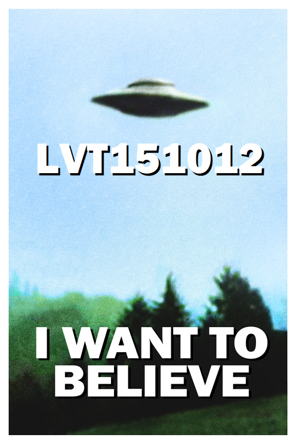
This paper describes the compact binary coalescence search pipelines and their results. As well as GW150914 there is also another interesting event, LVT151012. This isn’t significant enough to be claimed as a detection, but it is worth considering in more detail.
More details: The Compact Binary Coalescence Paper summary
3. The Parameter Estimation Paper
Title: Properties of the binary black hole merger GW150914
arXiv: 1602.03840 [gr-qc]
Journal: Physical Review Letters; 116(24):241102(19); 2016
LIGO science summary: The first measurement of a black hole merger and what it means
If you’re interested in the properties of the binary black hole system, then this is the paper for you! Here we explain how we do parameter estimation and how it is possible to extract masses, spins, location, etc. from the signal. These are the results I’ve been most heavily involved with, so I hope lots of people will find them useful! This is the paper to cite if you’re using our best masses, spins, distance or sky maps. The masses we infer are so large we conclude that the system must contain black holes, which is discovery (ii) reported in the Discovery Paper.
More details: The Parameter Estimation Paper summary
4. The Testing General Relativity Paper
Title: Tests of general relativity with GW150914
arXiv: 1602.03841 [gr-qc]
Journal: Physical Review Letters; 116(22):221101(19); 2016
LIGO science summary: Was Einstein right about strong gravity?
The observation of GW150914 provides a new insight into the behaviour of gravity. We have never before probed such strong gravitational fields or such highly dynamical spacetime. These are the sorts of places you might imagine that we could start to see deviations from the predictions of general relativity. Aside from checking that we understand gravity, we also need to check to see if there is any evidence that our estimated parameters for the system could be off. We find that everything is consistent with general relativity, which is good for Einstein and is also discovery (iii) in the Discovery Paper.
More details: The Testing General Relativity Paper summary
5. The Rates Paper
Title: The rate of binary black hole mergers inferred from Advanced LIGO observations surrounding GW150914
arXiv: 1602.03842 [astro-ph.HE]; 1606.03939 [astro-ph.HE]
Journal: Astrophysical Journal Letters; 833(1):L1(8); 2016; Astrophysical Journal Supplement Series; 227(2):14(11); 2016
LIGO science summary: The first measurement of a black hole merger and what it means
Given that we’ve spotted one binary black hole (plus maybe another with LVT151012), how many more are out there and how many more should we expect to find? We answer this here, although there’s a large uncertainty on the estimates since we don’t know (yet) the distribution of masses for binary black holes.
More details: The Rates Paper summary
6. The Burst Paper
Title: Observing gravitational-wave transient GW150914 with minimal assumptions
arXiv: 1602.03843 [gr-qc]
Journal: Physical Review D; 93(12):122004(20); 2016
What can you learn about GW150914 without having to make the assumptions that it corresponds to gravitational waves from a binary black hole merger (as predicted by general relativity)? This paper describes and presents the results of the burst searches. Since the pipeline which first found GW150914 was a burst pipeline, it seems a little unfair that this paper comes after the Compact Binary Coalescence Paper, but I guess the idea is to first present results assuming it is a binary (since these are tightest) and then see how things change if you relax the assumptions. The waveforms reconstructed by the burst models do match the templates for a binary black hole coalescence.
More details: The Burst Paper summary
7. The Detector Characterisation Paper
Title: Characterization of transient noise in Advanced LIGO relevant to gravitational wave signal GW150914
arXiv: 1602.03844 [gr-qc]
Journal: Classical & Quantum Gravity; 33(13):134001(34); 2016
LIGO science summary: How do we know GW150914 was real? Vetting a Gravitational Wave Signal of Astrophysical Origin
CQG+ post: How do we know LIGO detected gravitational waves? [featuring awesome cartoons]
Could GW150914 be caused by something other than a gravitational wave: are there sources of noise that could mimic a signal, or ways that the detector could be disturbed to produce something that would be mistaken for a detection? This paper looks at these problems and details all the ways we monitor the detectors and the external environment. We can find nothing that can explain GW150914 (and LVT151012) other than either a gravitational wave or a really lucky random noise fluctuation. I think this paper is extremely important to our ability to claim a detection and I’m surprised it’s not number 2 in the list of companion papers. If you want to know how thorough the Collaboration is in monitoring the detectors, this is the paper for you.
More details: The Detector Characterisation Paper summary
8. The Calibration Paper
Title: Calibration of the Advanced LIGO detectors for the discovery of the binary black-hole merger GW150914
arXiv: 1602.03845 [gr-qc]
Journal: Physical Review D; 95(6):062003(16); 2017
LIGO science summary: Calibration of the Advanced LIGO detectors for the discovery of the binary black-hole merger GW150914
Completing the triumvirate of instrumental papers with the Detector Paper and the Detector Characterisation Paper, this paper describes how the LIGO detectors are calibrated. There are some cunning control mechanisms involved in operating the interferometers, and we need to understand these to quantify how they effect what we measure. Building a better model for calibration uncertainties is high on the to-do list for improving parameter estimation, so this is an interesting area to watch for me.
More details: The Calibration Paper summary
9. The Astrophysics Paper
Title: Astrophysical implications of the binary black-hole merger GW150914
arXiv: 1602.03846 [astro-ph.HE]
Journal: Astrophysical Journal Letters; 818(2):L22(15); 2016
LIGO science summary: The first measurement of a black hole merger and what it means
Having estimated source parameters and rate of mergers, what can we say about astrophysics? This paper reviews results related to binary black holes to put our findings in context and also makes statements about what we could hope to learn in the future.
More details: The Astrophysics Paper summary
10. The Stochastic Paper
Title: GW150914: Implications for the stochastic gravitational wave background from binary black holes
arXiv: 1602.03847 [gr-qc]
Journal: Physical Review Letters; 116(13):131102(12); 2016
LIGO science summary: Background of gravitational waves expected from binary black hole events like GW150914
For every loud signal we detect, we expect that there will be many more quiet ones. This paper considers how many quiet binary black hole signals could add up to form a stochastic background. We may be able to see this background as the detectors are upgraded, so we should start thinking about what to do to identify it and learn from it.
More details: The Stochastic Paper summary
11. The Neutrino Paper
Title: High-energy neutrino follow-up search of gravitational wave event GW150914 with ANTARES and IceCube
arXiv: 1602.05411 [astro-ph.HE]
Journal: Physical Review D; 93(12):122010(15); 2016
LIGO science summary: Search for neutrinos from merging black holes
We are interested so see if there’s any other signal that coincides with a gravitational wave signal. We wouldn’t expect something to accompany a black hole merger, but it’s good to check. This paper describes the search for high-energy neutrinos. We didn’t find anything, but perhaps we will in the future (perhaps for a binary neutron star merger).
More details: The Neutrino Paper summary
12. The Electromagnetic Follow-up Paper
Title: Localization and broadband follow-up of the gravitational-wave transient GW150914
arXiv: 1602.08492 [astro-ph.HE]; 1604.07864 [astro-ph.HE]
Journal: Astrophysical Journal Letters; 826(1):L13(8); 2016; Astrophysical Journal Supplement Series; 225(1):8(15); 2016
As well as looking for coincident neutrinos, we are also interested in electromagnetic observations (gamma-ray, X-ray, optical, infra-red or radio). We had a large group of observers interesting in following up on gravitational wave triggers, and 25 teams have reported observations. This companion describes the procedure for follow-up observations and discusses sky localisation.
This work split into a main article and a supplement which goes into more technical details.
More details: The Electromagnetic Follow-up Paper summary
The Discovery Paper
Synopsis: Discovery Paper
Read this if: You want an overview of The Event
Favourite part: The entire conclusion:
The LIGO detectors have observed gravitational waves from the merger of two stellar-mass black holes. The detected waveform matches the predictions of general relativity for the inspiral and merger of a pair of black holes and the ringdown of the resulting single black hole. These observations demonstrate the existence of binary stellar-mass black hole systems. This is the first direct detection of gravitational waves and the first observation of a binary black hole merger.
The Discovery Paper gives the key science results and is remarkably well written. It seems a shame to summarise it: you should read it for yourself! (It’s free).
The Detector Paper
Synopsis: Detector Paper
Read this if: You want a brief description of the detector configuration for O1
Favourite part: It’s short!
The LIGO detectors contain lots of cool pieces of physics. This paper briefly outlines them all: the mirror suspensions, the vacuum (the LIGO arms are the largest vacuum envelopes in the world and some of the cleanest), the mirror coatings, the laser optics and the control systems. A full description is given in the Advanced LIGO paper, but the specs there are for design sensitivity (it is also heavy reading). The main difference between the current configuration and that for design sensitivity is the laser power. Currently the circulating power in the arms is  , the plan is to go up to
  . This will reduce shot noise, but raises all sorts of control issues, such as how to avoid parametric instabilities.

The noise amplitude spectral density. The curves for the current observations are shown in red (dark for Hanford, light for Livingston). This is around a factor 3 better than in the final run of initial LIGO (green), but still a factor of 3 off design sensitivity (dark blue). The light blue curve shows the impact of potential future upgrades. The improvement at low frequencies is especially useful for high-mass systems like GW150914. Part of Fig. 1 of the Detector Paper.
The Compact Binary Coalescence Paper
Synopsis: Compact Binary Coalescence Paper
Read this if: You are interested in detection significance or in LVT151012
Favourite part: We might have found a second binary black hole merger
There are two compact binary coalescence searches that look for binary black holes: PyCBC and GstLAL. Both match templates to the data from the detectors to look for anything binary like, they then calculate the probability that such a match would happen by chance due to a random noise fluctuation (the false alarm probability or p-value [unhappy bonus note]). The false alarm probability isn’t the probability that there is a gravitational wave, but gives a good indication of how surprised we should be to find this signal if there wasn’t one. Here we report the results of both pipelines on the first 38.6 days of data (about 17 days where both detectors were working at the same time).
Both searches use the same set of templates to look for binary black holes [bonus note]. They look for where the same template matches the data from both detectors within a time interval consistent with the travel time between the two. However, the two searches rank candidate events and calculate false alarm probabilities using different methods. Basically, both searches use a detection statistic (the quantity used to rank candidates: higher means less likely to be noise), that is based on the signal-to-noise ratio (how loud the signal is) and a goodness-of-fit statistic. They assess the significance of a particular value of this detection statistic by calculating how frequently this would be obtained if there was just random noise (this is done by comparing data from the two detectors when there is not a coincident trigger in both). Consistency between the two searches gives us greater confidence in the results.
PyCBC’s detection statistic is a reweighted signal-to-noise ratio  which takes into account the consistency of the signal in different frequency bands. You can get a large signal-to-noise ratio from a loud glitch, but this doesn’t match the template across a range of frequencies, which is why this test is useful. The consistency is quantified by a reduced chi-squared statistic. This is used, depending on its value, to weight the signal-to-noise ratio. When it is large (indicating inconsistency across frequency bins), the reweighted signal-to-noise ratio becomes smaller.
To calculate the background, PyCBC uses time slides. Data from the two detectors are shifted in time so that any coincidences can’t be due to a real gravitational wave. Seeing how often you get something signal-like then tells you how often you’d expect this to happen due to random noise.
GstLAL calculates the signal-to-noise ratio and a residual after subtracting the template. As a detection statistic, it uses a likelihood ratio  : the probability of finding the particular values of the signal-to-noise ratio and residual in both detectors for signals (assuming signal sources are uniformly distributed isotropically in space), divided by the probability of finding them for noise.
The background from GstLAL is worked out by looking at the likelihood ratio fro triggers that only appear in one detector. Since there’s no coincident signal in the other, these triggers can’t correspond to a real gravitational wave. Looking at their distribution tells you how frequently such things happen due to noise, and hence how probable it is for both detectors to see something signal-like at the same time.
The results of the searches are shown in the figure below.
GW150914 is the most significant event in both searches (it is the most significant PyCBC event even considering just single-detector triggers). They both find GW150914 with the same template values. The significance is literally off the charts. PyCBC can only calculate an upper bound on the false alarm probability of  . GstLAL calculates a false alarm probability of
  , but this is reaching the level that we have to worry about the accuracy of assumptions that go into this (that the distribution of noise triggers in uniform across templates—if this is not the case, the false alarm probability could be about
  times larger). Therefore, for our overall result, we stick to the upper bound, which is consistent with both searches. The false alarm probability is so tiny, I don’t think anyone doubts this signal is real.
There is a second event that pops up above the background. This is LVT151012. It is found by both searches. Its signal-to-noise ratio is  , compared with GW150914’s
  , so it is quiet. The false alarm probability from PyCBC is
  , and from GstLAL is
  , consistent with what we would expect for such a signal. LVT151012 does not reach the standards we would like to claim a detection, but it is still interesting.
Running parameter estimation on LVT151012, as we did for GW150914, gives beautiful results. If it is astrophysical in origin, it is another binary black hole merger. The component masses are lower,  and
and  (the asymmetric uncertainties come from imposing
  ); the chirp mass is
  . The effective spin, as for GW150914, is close to zero
  . The luminosity distance is
  , meaning it is about twice as far away as GW150914’s source. I hope we’ll write more about this event in the future; there are some more details in the Rates Paper.
Is it random noise or is it a gravitational wave? LVT151012 remains a mystery. This candidate event is discussed in the Compact Binary Coalescence Paper (where it is found), the Rates Paper (which calculates the probability that it is extraterrestrial in origin), and the Detector Characterisation Paper (where known environmental sources fail to explain it). SPOILERS
The Parameter Estimation Paper
Synopsis: Parameter Estimation Paper
Read this if: You want to know the properties of GW150914’s source
Favourite part: We inferred the properties of black holes using measurements of spacetime itself!
The gravitational wave signal encodes all sorts of information about its source. Here, we explain how we extract this information to produce probability distributions for the source parameters. I wrote about the properties of GW150914 in my previous post, so here I’ll go into a few more technical details.
To measure parameters we match a template waveform to the data from the two instruments. The better the fit, the more likely it is that the source had the particular parameters which were used to generate that particular template. Changing different parameters has different effects on the waveform (for example, changing the distance changes the amplitude, while changing the relative arrival times changes the sky position), so we often talk about different pieces of the waveform containing different pieces of information, even though we fit the whole lot at once.

The shape of the gravitational wave encodes the properties of the source. This information is what lets us infer parameters. The example signal is GW150914. I made this explainer with Ban Farr and Nutsinee Kijbunchoo for the LIGO Magazine.
The waveform for a binary black hole merger has three fuzzily defined parts: the inspiral (where the two black holes orbit each other), the merger (where the black holes plunge together and form a single black hole) and ringdown (where the final black hole relaxes to its final state). Having waveforms which include all of these stages is a fairly recent development, and we’re still working on efficient ways of including all the effects of the spin of the initial black holes.
We currently have two favourite binary black hole waveforms for parameter estimation:
- The first we refer to as EOBNR, short for its proper name of SEOBNRv2_ROM_DoubleSpin. This is constructed by using some cunning analytic techniques to calculate the dynamics (known as effective-one-body or EOB) and tuning the results to match numerical relativity (NR) simulations. This waveform only includes the effects of spins aligned with the orbital angular momentum of the binary, so it doesn’t allow us to measure the effects of precession (wobbling around caused by the spins).
- The second we refer to as IMRPhenom, short for IMRPhenomPv2. This is constructed by fitting to the frequency dependence of EOB and NR waveforms. The dominant effects of precession of included by twisting up the waveform.
We’re currently working on results using a waveform that includes the full effects of spin, but that is extremely slow (it’s about half done now), so those results won’t be out for a while.
The results from the two waveforms agree really well, even though they’ve been created by different teams using different pieces of physics. This was a huge relief when I was first making a comparison of results! (We had been worried about systematic errors from waveform modelling). The consistency of results is partly because our models have improved and partly because the properties of the source are such that the remaining differences aren’t important. We’re quite confident that we’ve most of the parameters are reliably measured!
The component masses are the most important factor for controlling the evolution of the waveform, but we don’t measure the two masses independently. The evolution of the inspiral is dominated by a combination called the chirp mass, and the merger and ringdown are dominated by the total mass. For lighter mass systems, where we gets lots of inspiral, we measure the chirp mass really well, and for high mass systems, where the merger and ringdown are the loudest parts, we measure the total mass. GW150914 is somewhere in the middle. The probability distribution for the masses are shown below: we can compensate for one of the component masses being smaller if we make the other larger, as this keeps chirp mass and total mass about the same.
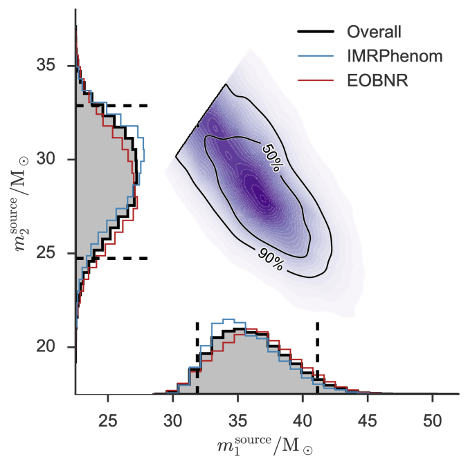
Estimated masses for the two black holes in the binary. Results are shown for the EOBNR waveform and the IMRPhenom: both agree well. The Overall results come from averaging the two. The dotted lines mark the edge of our 90% probability intervals. The sharp diagonal line cut-off in the two-dimensional plot is a consequence of requiring . Fig. 1 from the Parameter Estimation Paper.
To work out these masses, we need to take into account the expansion of the Universe. As the Universe expands, it stretches the wavelength of the gravitational waves. The same happens to light: visible light becomes redder, so the phenomenon is known as redshifting (even for gravitational waves). If you don’t take this into account, the masses you measure are too large. To work out how much redshift there is you need to know the distance to the source. The probability distribution for the distance is shown below, we plot the distance together with the inclination, since both of these affect the amplitude of the waves (the source is quietest when we look at it edge-on from the side, and loudest when seen face-on/off from above/below).

Estimated luminosity distance and binary inclination angle. An inclination of  means we are looking at the binary (approximately) edge-on. Results are shown for the EOBNR waveform and the IMRPhenom: both agree well. The Overall results come from averaging the two. The dotted lines mark the edge of our 90% probability intervals. Fig. 2 from the Parameter Estimation Paper.
After the masses, the most important properties for the evolution of the binary are the spins. We don’t measure these too well, but the probability distribution for their magnitudes and orientations from the precessing IMRPhenom model are shown below. Both waveform models agree that the effective spin  , which is a combination of both spins in the direction of the orbital angular momentum) is small. Therefore, either the spins are small or are larger but not aligned (or antialigned) with the orbital angular momentum. The spin of the more massive black hole is the better measured of the two.

Estimated orientation and magnitude of the two component spins from the precessing IMRPhenom model. The magnitude is between 0 and 1 and is perfectly aligned with the orbital angular momentum if the angle is 0. The distribution for the more massive black hole is on the left, and for the smaller black hole on the right. Part of Fig. 5 from the Parameter Estimation Paper.
The Testing General Relativity Paper
Synopsis: Testing General Relativity Paper
Read this if: You want to know more about the nature of gravity.
Favourite part: Einstein was right! (Or more correctly, we can’t prove he was wrong… yet)
The Testing General Relativity Paper is one of my favourites as it packs a lot of science in. Our first direct detection of gravitational waves and of the merger of two black holes provides a new laboratory to test gravity, and this paper runs through the results of the first few experiments.
Before we start making any claims about general relativity being wrong, we first have to check if there’s any weird noise present. You don’t want to have to rewrite the textbooks just because of an instrumental artifact. After taking out a good guess for the waveform (as predicted by general relativity), we find that the residuals do match what we expect for instrumental noise, so we’re good to continue.
I’ve written about a couple of tests of general relativity in my previous post: the consistency of the inspiral and merger–ringdown parts of the waveform, and the bounds on the mass of the graviton (from evolution of the signal). I’ll cover the others now.
The final part of the signal, where the black hole settles down to its final state (the ringdown), is the place to look to check that the object is a black hole and not some other type of mysterious dark and dense object. It is tricky to measure this part of the signal, but we don’t see anything odd. We can’t yet confirm that the object has all the properties you’d want to pin down that it is exactly a black hole as predicted by general relativity; we’re going to have to wait for a louder signal for this. This test is especially poignant, as Steven Detweiler, who pioneered a lot of the work calculating the ringdown of black holes, died a week before the announcement.
We can allow terms in our waveform (here based on the IMRPhenom model) to vary and see which values best fit the signal. If there is evidence for differences compared with the predictions from general relativity, we would have evidence for needing an alternative. Results for this analysis are shown below for a set of different waveform parameters  : the
: the  parameters determine the inspiral, the
  parameters determine the merger–ringdown and the
  parameters cover the intermediate regime. If the deviation
  is zero, the value coincides with the value from general relativity. The plot shows what would happen if you allow all the variable to vary at once (the multiple results) and if you tried just that parameter on its own (the single results).

Probability distributions for waveform parameters. The single analysis only varies one parameter, the multiple analysis varies all of them, and the J0737-3039 result is the existing bound from the double pulsar. A deviation of zero is consistent with general relativity. Fig. 7 from the Testing General Relativity Paper.
Overall the results look good. Some of the single results are centred away from zero, but we think that this is just a random fluctuate caused by noise (we’ve seen similar behaviour in tests, so don’t panic yet). It’s not surprising the  ,
,  and
and  all show this behaviour, as they are sensitive to similar noise features. These measurements are much tighter than from any test we’ve done before, except for the measurement of
  which is better measured from the double pulsar (since we have lots and lots of orbits of that measured).
The final test is to look for additional polarizations of gravitational waves. These are predicted in several alternative theories of gravity. Unfortunately, because we only have two detectors which are pretty much aligned we can’t say much, at least without knowing for certain the location of the source. Extra detectors will be useful here!
In conclusion, we have found no evidence to suggest we need to throw away general relativity, but future events will help us to perform new and stronger tests.
The Rates Paper
Synopsis: Rates Paper
Read this if: You want to know how often binary black holes merge (and how many we’ll detect)
Favourite part: There’s a good chance we’ll have ten detections by the end of our second observing run (O2)
Before September 14, we had never seen a binary stellar-mass black hole system. We were therefore rather uncertain about how many we would see. We had predictions based on simulations of the evolution of stars and their dynamical interactions. These said we shouldn’t be too surprised if we saw something in O1, but that we shouldn’t be surprised if we didn’t see anything for many years either. We weren’t really expecting to see a black hole system so soon (the smart money was on a binary neutron star). However, we did find a binary black hole, and this happened right at the start of our observations! What do we now believe about the rate of mergers?
To work out the rate, you first need to count the number of events you have detected and then work out how sensitive you are to the population of signals (how many could you see out of the total).
Counting detections sounds simple: we have GW150914 without a doubt. However, what about all the quieter signals? If you have 100 events each with a 1% probability of being real, then even though you can’t say with certainty that anyone is an actual signal, you would expect one to be so. We want to work out how many events are real and how many are due to noise. Handily, trying to tell apart different populations of things when you’re not certain about individual members is a common problem is astrophysics (where it’s often difficult to go and check what something actually is), so there exists a probabilistic framework for doing this.
Using the expected number of real and noise events for a given detection statistic (as described in the Compact Binary Coalescence Paper), we count the number of detections and as a bonus, get a probability that each event is of astrophysical origin. There are two events with more than a 50% chance of being real: GW150914, where the probability is close to 100%, and LVT151012, where to probability is 84% based on GstLAL and 91% based on PyCBC.
By injecting lots of fake signals into some data and running our detection pipelines, we can work out how sensitive they are (in effect, how far away can they find particular types of sources). For a given number of detections, the more sensitive we are, the lower the actual rate of mergers should be (for lower sensitivity we would miss more, while there’s no hiding for higher sensitivity).
There is one final difficulty in working out the total number of binary black hole mergers: we need to know the distribution of masses, because our sensitivity depends on this. However, we don’t yet know this as we’ve only seen GW150914 and (maybe) LVT151012. Therefore, we try three possibilities to get an idea of what the merger rate could be.
- We assume that binary black holes are either like GW150914 or like LVT151012. Given that these are our only possible detections at the moment, this should give a reasonable estimate. A similar approach has been used for estimating the population of binary neutron stars from pulsar observations [bonus note].
- We assume that the distribution of masses is flat in the logarithm of the masses. This probably gives more heavy black holes than in reality (and so a lower merger rate)
- We assume that black holes follow a power law like the initial masses of stars. This probably gives too many low mass black holes (and so a higher merger rate)
The estimated merger rates (number of binary black hole mergers per volume per time) are then: 1.  ; 2.
; 2. 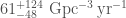 , and 3.
 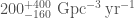 . There is a huge scatter, but the flat and power-law rates hopefully bound the true value.
We’ll pin down the rate better after a few more detections. How many more should we expect to see? Using the projected sensitivity of the detectors over our coming observing runs, we can work out the probability of making  more detections. This is shown in the plot below. It looks like there’s about about a 10% chance of not seeing anything else in O1, but we’re confident that we’ll have 10 more by the end of O2, and 35 more by the end of O3! I may need to lie down…

The percentage chance of making 0, 10, 35 and 70 more detections of binary black holes as time goes on and detector sensitivity improves (based upon our data so far). This is a simplified version of part of Fig. 3 of the Rates Paper taken from the science summary.
The Burst Paper
Synopsis: Burst Paper
Read this if: You want to check what we can do without a waveform template
Favourite part: You don’t need a template to make a detection
When discussing what we can learn from gravitational wave astronomy, you can almost guarantee that someone will say something about discovering the unexpected. Whenever we’ve looked at the sky in a new band of the electromagnetic spectrum, we found something we weren’t looking for: pulsars for radio, gamma-ray burst for gamma-rays, etc. Can we do the same in gravitational wave astronomy? There may well be signals we weren’t anticipating out there, but will we be able to detect them? The burst pipelines have our back here, at least for short signals.
The burst search pipelines, like their compact binary coalescence partners, assign candidate events a detection statistic and then work out a probability associated with being a false alarm caused by noise. The difference is that the burst pipelines try to find a wider range of signals.
There are three burst pipelines described: coherent WaveBurst (cWB), which famously first found GW150914; omicron–LALInferenceBurst (oLIB), and BayesWave, which follows up on cWB triggers.
As you might guess from the name, cWB looks for a coherent signal in both detectors. It looks for excess power (indicating a signal) in a time–frequency plot, and then classifies candidates based upon their structure. There’s one class for blip glitches and resonance lines (see the Detector Characterisation Paper), these are all thrown away as noise; one class for chirp-like signals that increase in frequency with time, this is where GW150914 was found, and one class for everything else. cWB’s detection statistic  is something like a signal-to-noise ratio constructed based upon the correlated power in the detectors. The value for GW150914 was
  , which is higher than for any other candidate. The false alarm probability (or p-value), folding in all three search classes, is
  , which is pretty tiny, even if not as significant as for the tailored compact binary searches.
The oLIB search has two stages. First it makes a time–frequency plot and looks for power coincident between the two detectors. Likely candidates are then followed up by matching a sine–Gaussian wavelet to the data, using a similar algorithm to the one used for parameter estimation. It’s detection statistic is something like a likelihood ratio for the signal verses noise. It calculates a false alarm probability of about too.
BayesWave fits a variable number of sine–Gaussian wavelets to the data. This can model both a signal (when the wavelets are the same for both detectors) and glitches (when the wavelets are independent). This is really clever, but is too computationally expensive to be left running on all the data. Therefore, it follows up on things highlighted by cWB, potentially increasing their significance. It’s detection statistic is the Bayes factor comparing the signal and glitch models. It estimates the false alarm probability to be about  (which agrees with the cWB estimate if you only consider chirp-like triggers).
None of the searches find LVT151012. However, as this is a quiet, lower mass binary black hole, I think that this is not necessarily surprising.
cWB and BayesWave also output a reconstruction of the waveform. Reassuringly, this does look like binary black hole coalescence!
Gravitational waveforms from our analyses of GW150914. The wiggly grey line are the data from Hanford (top) and Livinston (bottom); these are analysed coherently. The plots show waveforms whitened by the noise power spectral density. The dark band shows the waveform reconstructed by BayesWave without assuming that the signal is from a binary black hole (BBH). The light bands show the distribution of BBH template waveforms that were found to be most probable from our parameter-estimation analysis. The two techniques give consistent results: the match between the two models is  . Fig. 6 of the Parameter Estimation Paper.
The paper concludes by performing some simple fits to the reconstructed waveforms. For this, you do have to assume that the signal cane from a binary black hole. They find parameters roughly consistent with those from the full parameter-estimation analysis, which is a nice sanity check of our results.
The Detector Characterisation Paper
Synopsis: Detector Characteristation Paper
Read this if: You’re curious if something other than a gravitational wave could be responsible for GW150914 or LVT151012
Favourite part: Mega lightning bolts can cause correlated noise
The output from the detectors that we analyses for signals is simple. It is a single channel that records the strain. To monitor instrumental behaviour and environmental conditions the detector characterisation team record over 200,000 other channels. These measure everything from the alignment of the optics through ground motion to incidence of cosmic rays. Most of the data taken by LIGO is to monitor things which are not gravitational waves.
This paper examines all the potential sources of noise in the LIGO detectors, how we monitor them to ensure they are not confused for a signal, and the impact they could have on estimating the significance of events in our searches. It is amazingly thorough work.
There are lots of potential noise sources for LIGO. Uncorrelated noise sources happen independently at both sites, therefore they can only be mistaken for a gravitational wave if by chance two occur at the right time. Correlated noise sources effect both detectors, and so could be more confusing for our searches, although there’s no guarantee that they would cause a disturbance that looks anything like a binary black hole merger.
Sources of uncorrelated noise include:
- Ground motion caused by earthquakes or ocean waves. These create wibbling which can affect the instruments, even though they are well isolated. This is usually at low frequencies (below
 for earthquakes, although it can be higher if the epicentre is near), unless there is motion in the optics around (which can couple to cause higher frequency noise). There is a network of seismometers to measure earthquakes at both sites. There where two magnitude 2.1 earthquakes within 20 minutes of GW150914 (one off the coast of Alaska, the other south-west of Seattle), but both produced ground motion that is ten times too small to impact the detectors. There was some low frequency noise in Livingston at the time of LVT151012 which is associated with a period of bad ocean waves. however, there is no evidence that these could be converted to the frequency range associated with the signal.
- People moving around near the detectors can also cause vibrational or acoustic disturbances. People are kept away from the detectors while they are running and accelerometers, microphones and seismometers monitor the environment.
- Modulation of the lasers at
 and
and  is done to monitor and control several parts of the optics. There is a fault somewhere in the system which means that there is a coupling to the output channel and we get noise across
  to
to  , which is where we look for compact binary coalescences. Rai Weiss suggested shutting down the instruments to fix the source of this and delaying the start of observations—it’s a good job we didn’t. Periods of data where this fault occurs are flagged and not included in the analysis.
- Blip transients are a short glitch that occurs for unknown reasons. They’re quite mysterious. They are at the right frequency range (
 to
to  ) to be confused with binary black holes, but don’t have the right frequency evolution. They contribute to the background of noise triggers in the compact binary coalescence searches, but are unlikely to be the cause of GW150914 or LVT151012 since they don’t have the characteristic chirp shape.

A time–frequency plot of a blip glitch in LIGO-Livingston. Blip glitches are the right frequency range to be confused with binary coalescences, but don’t have the chirp-like structure. Blips are symmetric in time, whereas binary coalescences sweep up in frequency. Fig. 3 of the Detector Characterisation Paper.
Correlated noise can be caused by:
- Electromagnetic signals which can come from lightning, solar weather or radio communications. This is measured by radio receivers and magnetometers, and its extremely difficult to produce a signal that is strong enough to have any impact of the detectors’ output. There was one strong (peak current of about
 ) lightning strike in the same second as GW150914 over Burkino Faso. However, the magnetic disturbances were at least a thousand times too small to explain the amplitude of GW150914.
- Cosmic ray showers can cause electromagnetic radiation and particle showers. The particle flux become negligible after a few kilometres, so it’s unlikely that both Livingston and Hanford would be affected, but just in case there is a cosmic ray detector at Hanford. It has seen nothing suspicious.
All the monitoring channels give us a lot of insight into the behaviour of the instruments. Times which can be identified as having especially bad noise properties (where the noise could influence the measured output), or where the detectors are not working properly, are flagged and not included in the search analyses. Applying these vetoes mean that we can’t claim a detection when we know something else could mimic a gravitational wave signal, but it also helps us clean up our background of noise triggers. This has the impact of increasing the significance of the triggers which remain (since there are fewer false alarms they could be confused with). For example, if we leave the bad period in, the PyCBC false alarm probability for LVT151012 goes up from to  . The significance of GW150914 is so great that we don’t really need to worry about the effects of vetoes.
At the time of GW150914 the detectors were running well, the data around the event are clean, and there is nothing in any of the auxiliary channels that record anything which could have caused the event. The only source of a correlated signal which has not been rules out is a gravitational wave from a binary black hole merger. The time–frequency plots of the measured strains are shown below, and its easy to pick out the chirps.

Time–frequency plots for GW150914 as measured by Hanford (left) and Livingston (right). These show the characteristic increase in frequency with time of the chirp of a binary merger. The signal is clearly visible above the noise. Fig. 10 of the Detector Characterisation Paper.
The data around LVT151012 are significantly less stationary than around GW150914. There was an elevated noise transient rate around this time. This is probably due to extra ground motion caused by ocean waves. This low frequency noise is clearly visible in the Livingston time–frequency plot below. There is no evidence that this gets converted to higher frequencies though. None of the detector characterisation results suggest that LVT151012 has was caused by a noise artifact.

Time–frequency plots for LVT151012 as measured by Hanford (left) and Livingston (right). You can see the characteristic increase in frequency with time of the chirp of a binary merger, but this is mixed in with noise. The scale is reduced compared with for GW150914, which is why noise features appear more prominent. The band at low frequency in Livingston is due to ground motion; this is not present in Hanford. Fig. 13 of the Detector Characterisation Paper.
If you’re curious about the state of the LIGO sites and their array of sensors, you can see more about the physical environment monitors at pem.ligo.org.
The Calibration Paper
Synopsis: Calibration Paper
Read this if: You like control engineering or precision measurement
Favourite part: Not only are the LIGO detectors sensitive enough to feel the push from a beam of light, they are so sensitive that you have to worry about where on the mirrors you push
We want to measure the gravitational wave strain—the change in length across our detectors caused by a passing gravitational wave. What we actually record is the intensity of laser light out the output of our interferometer. (The output should be dark when the strain is zero, and the intensity increases when the interferometer is stretched or squashed). We need a way to convert intensity to strain, and this requires careful calibration of the instruments.
The calibration is complicated by the control systems. The LIGO instruments are incredibly sensitive, and maintaining them in a stable condition requires lots of feedback systems. These can impact how the strain is transduced into the signal readout by the interferometer. A schematic of how what would be the change in the length of the arms without control systems  is changed into the measured strain
  is shown below. The calibration pipeline build models to correct for the effects of the control system to provide an accurate model of the true gravitational wave strain.
To measure the different responses of the system, the calibration team make several careful measurements. The primary means is using photon calibration: an auxiliary laser is used to push the mirrors and the response is measured. The spots where the lasers are pointed are carefully chosen to minimise distortion to the mirrors caused by pushing on them. A secondary means is to use actuators which are parts of the suspension system to excite the system.
As a cross-check, we can also use two auxiliary green lasers to measure changes in length using either a frequency modulation or their wavelength. These are similar approaches to those used in initial LIGO. These go give consistent results with the other methods, but they are not as accurate.
Overall, the uncertainty in the calibration of the amplitude of the strain is less than  between
  and
and  , and the uncertainty in phase calibration is less than
  . These are the values that we use in our parameter-estimation runs. However, the calibration uncertainty actually varies as a function of frequency, with some ranges having much less uncertainty. We’re currently working on implementing a better model for the uncertainty, which may improve our measurements. Fortunately the masses, aren’t too affected by the calibration uncertainty, but sky localization is, so we might get some gain here. We’ll hopefully produce results with updated calibration in the near future.
The Astrophysics Paper
Synopsis: Astrophysics Paper
Read this if: You are interested in how binary black holes form
Favourite part: We might be able to see similar mass binary black holes with eLISA before they merge in the LIGO band [bonus note]
This paper puts our observations of GW150914 in context with regards to existing observations of stellar-mass black holes and theoretical models for binary black hole mergers. Although it doesn’t explicitly mention LVT151012, most of the conclusions would be just as applicable to it’s source, if it is real. I expect there will be rapid development of the field now, but if you want to catch up on some background reading, this paper is the place to start.
The paper contains lots of references to good papers to delve into. It also highlights the main conclusion we can draw in italics, so its easy to skim through if you want a summary. I discussed the main astrophysical conclusions in my previous post. We will know more about binary black holes and their formation when we get more observations, so I think it is a good time to get interested in this area.
The Stochastic Paper
Synopsis: Stochastic Paper
Read this if: You like stochastic backgrounds
Favourite part: We might detect a background in the next decade
A stochastic gravitational wave background could be created by an incoherent superposition of many signals. In pulsar timing, they are looking for a background from many merging supermassive black holes. Could we have a similar thing from stellar-mass black holes? The loudest signals, like GW150914, are resolvable, they stand out from the background. However, for every loud signal, there will be many quiet signals, and the ones below our detection threshold could form a background. Since we’ve found that binary black hole mergers are probably plentiful, the background may be at the high end of previous predictions.
The background from stellar-mass black holes is different than the one from supermassive black holes because the signals are short. While the supermassive black holes produce an almost constant hum throughout your observations, stellar-mass black hole mergers produce short chirps. Instead of having lots of signals that overlap in time, we have a popcorn background, with one arriving on average every 15 minutes. This might allow us to do some different things when it comes to detection, but for now, we just use the standard approach.
This paper calculates the energy density of gravitational waves from binary black holes, excluding the contribution from signals loud enough to be detected. This is done for several different models. The standard (fiducial) model assumes parameters broadly consistent with those of GW150914’s source, plus a particular model for the formation of merging binaries. There are then variations on the the model for formation, considering different time delays between formation and merger, and adding in lower mass systems consistent with LVT151012. All these models are rather crude, but give an idea of potential variations in the background. Hopefully more realistic distributions will be considered in the future. There is some change between models, but this is within the (considerable) statistical uncertainty, so predictions seems robust.

Different models for the stochastic background of binary black holes. This is plotted in terms of energy density. The red band indicates the uncertainty on the fiducial model. The dashed line indicates the sensitivity of the LIGO and Virgo detectors after several years at design sensitivity. Fig. 2 of the Stochastic Paper.
After a couple of years at design sensitivity we may be able to make a confident detection of the stochastic background. The background from binary black holes is more significant than we expected.
If you’re wondering about if we could see other types of backgrounds, such as one of cosmological origin, then the background due to binary black holes could make detection more difficult. In effect, it acts as another source of noise, masking the other background. However, we may be able to distinguish the different backgrounds by measuring their frequency dependencies (we expect them to have different slopes), if they are loud enough.
The Neutrino Paper
Synopsis: Neutrino Paper
Read this if: You really like high energy neutrinos
Favourite part: We’re doing astronomy with neutrinos and gravitational waves—this is multimessenger astronomy without any form of electromagnetic radiation
There are multiple detectors that can look for high energy neutrinos. Currently, LIGO–Virgo Observations are being followed up by searches from ANTARES and IceCube. Both of these are Cherenkov detectors: they look for flashes of light created by fast moving particles, not the neutrinos themselves, but things they’ve interacted with. ANTARES searches the waters of the Mediterranean while IceCube uses the ice of Antarctica.
Within 500 seconds either side of the time of GW150914, ANTARES found no neutrinos and IceCube found three. These results are consistent with background levels (you would expect on average less than one and 4.4 neutrinos over that time from the two respectively). Additionally, none of the IceCube neutrinos are consistent with the sky localization of GW150914 (even though the sky area is pretty big). There is no sign of a neutrino counterpart, which is what we were expecting.
Subsequent non-detections have been reported by KamLAND, the Pierre Auger Observatory, Super-Kamiokande, Borexino and NOvA.
The Electromagnetic Follow-up Paper
Synopsis: Electromagnetic Follow-up Paper
Read this if: You are interested in the search for electromagnetic counterparts
Favourite part: So many people were involved in this work that not only do we have to abbreviate the list of authors (Abbott, B.P. et al.), but we should probably abbreviate the list of collaborations too (LIGO Scientific & Virgo Collaboration et al.)
This is the last of the set of companion papers to be released—it took a huge amount of coordinating because of all the teams involved. The paper describes how we released information about GW150914. This should not be typical of how we will do things going forward (i) because we didn’t have all the infrastructure in place on September 14 and (ii) because it was the first time we had something we thought was real.
The first announcement was sent out on September 16, and this contained sky maps from the Burst codes cWB and LIB. In the future, we should be able to send out automated alerts with a few minutes latency.
For the first alert, we didn’t have any results which assumed the the source was a binary, as the searches which issue triggers at low latency were only looking for lower mass systems which would contain a neutron star. I suspect we’ll be reprioritising things going forward. The first information we shared about the potential masses for the source was shared on October 3. Since this was the first detection, everyone was cautious about triple-checking results, which caused the delay. Revised false alarm rates including results from GstLAL and PyCBC were sent out October 20.
The final sky maps were shared January 13. This is when we’d about finished our own reviews and knew that we would be submitting the papers soon [bonus note]. Our best sky map is the one from the Parameter Estimation Paper. You might it expect to be more con straining than the results from the burst pipelines since it uses a proper model for the gravitational waves from a binary black hole. This is the case if we ignore calibration uncertainty (which is not yet included in the burst codes), then the 50% area is  and the 90% area is
  . However, including calibration uncertainty, the sky areas are and
  at 50% and 90% probability respectively. Calibration uncertainty has the largest effect on sky area. All the sky maps agree that the source is in in some region of the annulus set by the time delay between the two detectors.

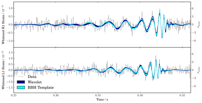
The different sky maps for GW150914 in an orthographic projection. The contours show the 90% region for each algorithm. The faint circles show lines of constant time delay  between the two detectors. BAYESTAR rapidly computes sky maps for binary coalescences, but it needs the output of one of the detection pipelines to run, and so was not available at low latency. The LALInference map is our best result. All the sky maps are available as part of the data release. Fig. 2 of the Electromagnetic Follow-up Paper.
A timeline of events is shown below. There were follow-up observations across the electromagnetic spectrum from gamma-rays and X-rays through the optical and near infra-red to radio.

Timeline for observations of GW15014. The top (grey) band shows information about gravitational waves. The second (blue) band shows high-energy (gamma- and X-ray) observations. The third and fourth (green) bands show optical and near infra-red observations respectively. The bottom (red) band shows radio observations. Fig. 1 from the Electromagnetic Follow-up Paper.
Observations have been reported (via GCN notices) by
Together they cover an impressive amount of the sky as shown below. Many targeted the Large Magellanic Cloud before the knew the source was a binary black hole.
Footprints of observations compared with the 50% and 90% areas of the initially distributed (cWB: thick lines; LIB: thin lines) sky maps, also in orthographic projection. The all-sky observations are not shown. The grey background is the Galactic plane. Fig. 3 of the Electromagnetic Follow-up Paper.
Additional observations have been done using archival data by XMM-Newton and AGILE.
We don’t expect any electromagnetic counterpart to a binary black hole. No-one found anything with the exception of Fermi GBM. This has found a weak signal which may be coincident. More work is required to figure out if this is genuine (the statistical analysis looks OK, but some times you do have a false alarm). It would be a surprise if it is, so most people are sceptical. However, I think this will make people more interested in following up on our next binary black hole signal!
Bonus notes
Naming The Event
GW150914 is the name we have given to the signal detected by the two LIGO instruments. The “GW” is short for gravitational wave (not galactic worm), and the numbers give the date the wave reached the detectors (2015 September 14). It was originally known as G184098, its ID in our database of candidate events (most circulars sent to and from our observer partners use this ID). That was universally agreed to be terrible to remember. We tried to think of a good nickname for the event, but failed to, so rather by default, it has informally become known as The Event within the Collaboration. I think this is fitting given its significance.
LVT151012 is the name of the most significant candidate after GW150914, it doesn’t reach our criteria to claim detection (a false alarm rate of less than once per century), which is why it’s not GW151012. The “LVT” is short for LIGO–Virgo trigger. It took a long time to settle on this and up until the final week before the announcement it was still going by G197392. Informally, it was known as The Second Monday Event, as it too was found on a Monday. You’ll have to wait for us to finish looking at the rest of the O1 data to see if the Monday trend continues. If it does, it could have serious repercussions for our understanding of Garfield.
Following the publication of the O2 Catalogue Paper, LVT151012 was upgraded to GW151012, AND we decided to get rid of the LVT class as it was rather confusing.
Publishing in Physical Review Letters
Several people have asked me if the Discovery Paper was submitted to Science or Nature. It was not. The decision that any detection would be submitted to Physical Review was made ahead of the run. As far as I am aware, there was never much debate about this. Physical Review had been good about publishing all our non-detections and upper limits, so it only seemed fair that they got the discovery too. You don’t abandon your friends when you strike it rich. I am glad that we submitted to them.
Gaby González, the LIGO Spokesperson, contacted the editors of Physical Review Letters ahead of submission to let them know of the anticipated results. They then started to line up some referees to give confidential and prompt reviews.
The initial plan was to submit on January 19, and we held a Collaboration-wide tele-conference to discuss the science. There were a few more things still to do, so the paper was submitted on January 21, following another presentation (and a long discussion of whether a number should be a six or a two) and a vote. The vote was overwhelmingly in favour of submission.
We got the referee reports back on January 27, although they were circulated to the Collaboration the following day. This was a rapid turnaround! From their comments, I suspect that Referee A may be a particle physicist who has dealt with similar claims of first detection—they were most concerned about statistical significance; Referee B seemed like a relativist—they made comments about the effect of spin on measurements, knew about waveforms and even historical papers on gravitational waves, and I would guess that Referee C was an astronomer involved with pulsars—they mentioned observations of binary pulsars potentially claiming the title of first detection and were also curious about sky localization. While I can’t be certain who the referees were, I am certain that I have never had such positive reviews before! Referee A wrote
The paper is extremely well written and clear. These results are obviously going to make history.
Referee B wrote
This paper is a major breakthrough and a milestone in gravitational science. The results are overall very well presented and its suitability for publication in Physical Review Letters is beyond question.
and Referee C wrote
It is an honor to have the opportunity to review this paper. It would not be an exaggeration to say that it is the most enjoyable paper I’ve ever read. […] I unreservedly recommend the paper for publication in Physical Review Letters. I expect that it will be among the most cited PRL papers ever.
I suspect I will never have such emphatic reviews again [happy bonus note][unhappy bonus note].
Publishing in Physical Review Letters seems to have been a huge success. So much so that their servers collapsed under the demand, despite them adding two more in anticipation. In the end they had to quintuple their number of servers to keep up with demand. There were 229,000 downloads from their website in the first 24 hours. Many people remarked that it was good that the paper was freely available. However, we always make our papers public on the arXiv or via LIGO’s Document Control Center [bonus bonus note], so there should never be a case where you miss out on reading a LIGO paper!
Publishing the Parameter Estimation Paper
The reviews for the Parameter Estimation Paper were also extremely positive. Referee A, who had some careful comments on clarifying notation, wrote
This is a beautiful paper on a spectacular result.
Referee B, who commendably did some back-of-the-envelope checks, wrote
The paper is also very well written, and includes enough background that I think a decent fraction of it will be accessible to non-experts. This, together with the profound nature of the results (first direct detection of gravitational waves, first direct evidence that Kerr black holes exist, first direct evidence that binary black holes can form and merge in a Hubble time, first data on the dynamical strong-field regime of general relativity, observation of stellar mass black holes more massive than any observed to date in our galaxy), makes me recommend this paper for publication in PRL without hesitation.
Referee C, who made some suggestions to help a non-specialist reader, wrote
This is a generally excellent paper describing the properties of LIGO’s first detection.
Physical Review Letters were also kind enough to publish this paper open access without charge!
Publishing the Rates Paper
It wasn’t all clear sailing getting the companion papers published. Referees did give papers the thorough checking that they deserved. The most difficult review was of the Rates Paper. There were two referees, one astrophysics, one statistics. The astrophysics referee was happy with the results and made a few suggestions to clarify or further justify the text. The statistics referee has more serious complaints…
There are five main things which I think made the statistics referee angry. First, the referee objected to our terminology
While overall I’ve been impressed with the statistics in LIGO papers, in one respect there is truly egregious malpractice, but fortunately easy to remedy. It concerns incorrectly using the term “false alarm probability” (FAP) to refer to what statisticians call a p-value, a deliberately vague term (“false alarm rate” is similarly misused). […] There is nothing subtle or controversial about the LIGO usage being erroneous, and the practice has to stop, not just within this paper, but throughout the LIGO collaboration (and as a matter of ApJ policy).
I agree with this. What we call the false alarm probability is not the probability that the detection is a false alarm. It is not the probability that the given signal is noise rather that astrophysical, but instead it is the probability that if we only had noise that we would get a detection statistic as significant or more so. It might take a minute to realise why those are different. The former (the one we should call p-value) is what the search pipelines give us, but is less useful than the latter for actually working out if the signal is real. The probabilities calculated in the Rates Paper that the signal is astrophysical are really what you want.
p-values are often misinterpreted, but most scientists are aware of this, and so are cautious when they come across them
As a consequence of this complaint, the Collaboration is purging “false alarm probability” from our papers. It is used in most of the companion papers, as they were published before we got this report (and managed to convince everyone that it is important).
Second, we were lacking in references to existing literature
Regarding scholarship, the paper is quite poor. I take it the authors have written this paper with the expectation, or at least the hope, that it would be read […] If I sound frustrated, it’s because I am.
This is fair enough. The referee made some good suggestions to work done on inferring the rate of gamma-ray bursts by Loredo & Wasserman (Part I, Part II, Part III), as well as by Petit, Kavelaars, Gladman & Loredo on trans-Neptunian objects, and we made sure to add as much work as possible in revisions. There’s no excuse for not properly citing useful work!
Third, the referee didn’t understand how we could be certain of the distribution of signal-to-noise ratio  without also worrying about the distribution of parameters like the black hole masses. The signal-to-noise ratio is inversely proportional to distance, and we expect sources to be uniformly distributed in volume. Putting these together (and ignoring corrections from cosmology) gives a distribution for signal-to-noise ratio of
  (Schulz 2011). This is sufficiently well known within the gravitational-wave community that we forgot that those outside wouldn’t appreciate it without some discussion. Therefore, it was useful that the referee did point this out.
Fourth, the referee thought we had made an error in our approach. They provided an alternative derivation which
if useful, should not be used directly without some kind of attribution
Unfortunately, they were missing some terms in their expressions. When these were added in, their approach reproduced our own (I had a go at checking this myself). Given that we had annoyed the referee on so many other points, it was tricky trying to convince them of this. Most of the time spent responding to the referees was actually working on the referee response and not on the paper.
Finally, the referee was unhappy that we didn’t make all our data public so that they could check things themselves. I think it would be great, and it will happen, it was just too early at the time.
LIGO Document Control Center
Papers in the LIGO Document Control Center are assigned a number starting with P (for “paper”) and then several digits. The Discover Paper’s reference is P150914. I only realised why this was the case on the day of submission.
The überbank
The set of templates used in the searches is designed to be able to catch binary neutron stars, neutron star–black hole binaries and binary neutron stars. It covers component masses from 1 to 99 solar masses, with total masses less than 100 solar masses. The upper cut off is chosen for computational convenience, rather than physical reasons: we do look for higher mass systems in a similar way, but they are easier to confuse with glitches and so we have to be more careful tuning the search. Since bank of templates is so comprehensive, it is known as the überbank. Although it could find binary neutron stars or neutron star–black hole binaries, we only discuss binary black holes here.
The template bank doesn’t cover the full parameter space, in particular it assumes that spins are aligned for the two components. This shouldn’t significantly affect its efficiency at finding signals, but gives another reason (together with the coarse placement of templates) why we need to do proper parameter estimation to measure properties of the source.
Alphabet soup
In the calculation of rates, the probabilistic means for counting sources is known as the FGMC method after its authors (who include two Birmingham colleagues and my former supervisor). The means of calculating rates assuming that the population is divided into one class to match each observation is also named for the initial of its authors as the KKL approach. The combined FGMCKKL method for estimating merger rates goes by the name alphabet soup, as that is much easier to swallow.
Multi-band gravitational wave astronomy
The prospect of detecting a binary black hole with a space-based detector and then seeing the same binary merger with ground-based detectors is especially exciting. My officemate Alberto Sesana (who’s not in LIGO) has just written a paper on the promise of multi-band gravitational wave astronomy. Black hole binaries like GW150914 could be spotted by eLISA (if you assume one of the better sensitivities for a detector with three arms). Then a few years to weeks later they merge, and spend their last moments emitting in LIGO’s band. The evolution of some binary black holes is sketched in the plot below.

The evolution of binary black hole mergers (shown in blue). The eLISA and Advanced LIGO sensitivity curves are shown in purple and orange respectively. As the black holes inspiral, they emit gravitational waves at higher frequency, shifting from the eLISa band to the LIGO band (where they merge). The scale at the top gives the approximate time until merger. Fig. 1 of Sesana (2016).
Seeing the signal in two bands can help in several ways. First it can increase our confidence in detection, potentially picking out signals that we wouldn’t otherwise. Second, it gives us a way to verify the calibration of our instruments. Third, it lets us improve our parameter-estimation precision—eLISA would see thousands of cycles, which lets it pin down the masses to high accuracy, these results can be combined with LIGO’s measurements of the strong-field dynamics during merger to give a fantastic overall picture of the system. Finally, since eLISA can measure the signal for a considerable time, it can well localise the source, perhaps just to a square degree; since we’ll also be able to predict when the merger will happen, you can point telescopes at the right place ahead of time to look for any electromagnetic counterparts which may exist. Opening up the gravitational wave spectrum is awesome!
The LALInference sky map
One of my jobs as part of the Parameter Estimation group was to produce the sky maps from our parameter-estimation runs. This is a relatively simple job of just running our sky area code. I had done it many times while were collecting our results, so I knew that the final versions were perfectly consistent with everything else we had seen. While I was comfortable with running the code and checking the results, I was rather nervous uploading the results to our database to be shared with our observational partners. I somehow managed to upload three copies by accident. D’oh! Perhaps future historians will someday look back at the records for G184098/GW150914 and wonder what was this idiot Christopher Berry doing? Probably no-one would every notice, but I know the records are there…


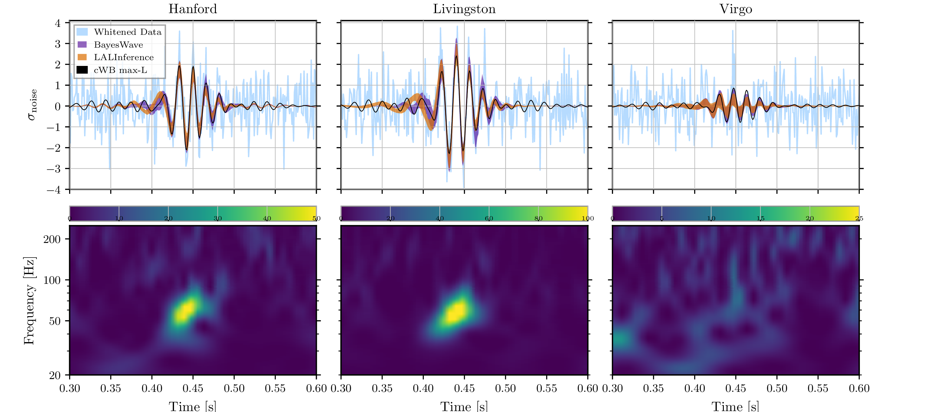

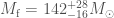


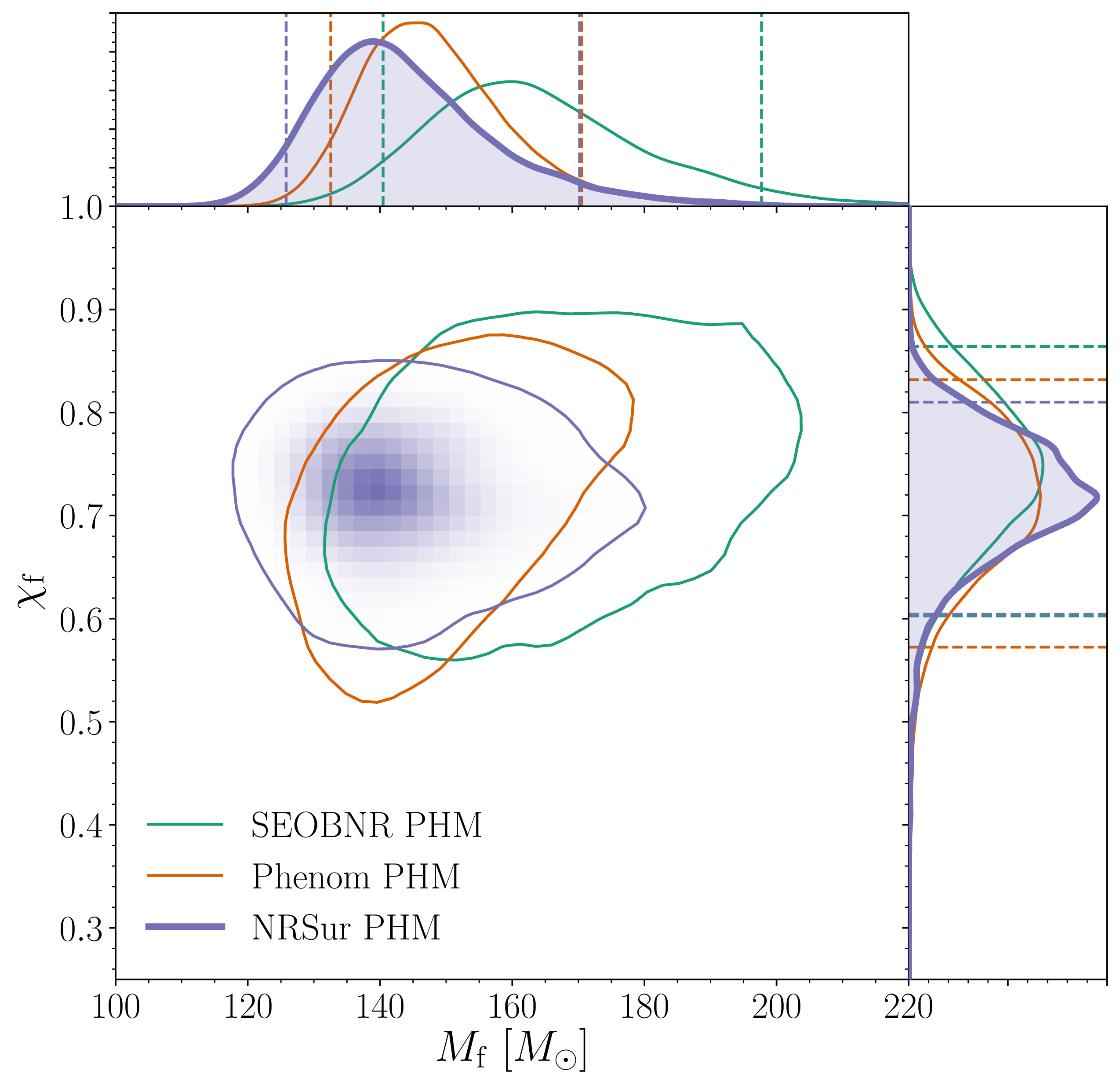


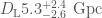


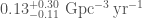


 times the mass of our Sun (quoting the 90% range for parameters), and the other
  times the mass of our Sun. Neither of these masses is too surprising on their own. We know black holes come in these sizes. What is new is the ratio of the masses
 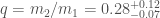 [
[
 for the two components in the binary and the effective inspiral spin
  ,
, and
and  are the spins of the two black holes [
 and
and  are the tilts angles measuring the alignment of the spins with the orbital angular momentum. The spins change orientations during the inspiral if they are not perfectly aligned with the orbital angular momentum, which is referred to as precession, but
 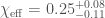 .
. .
. . This is the best measurement of
 ), and similarly
  ). Combining all this information, we can actually get a good measurement of the spin of the bigger black hole. We infer that
  . This is the first time we’ve really been able to measure an individual spin!
 , where we use
  as the angles on the sphere, and
  specify the harmonic. The majority of the gravitational radiation emitted from a binary is from the
  harmonic, so we usually start with this. Larger values of
  contribute less and less. For exactly equal mass binaries with non-spinning components, only harmonics with even
  are expected to contribute a significant amount. In previous detection, we’ve not had to worry too much about the harmonics with
  , which we refer to as higher order multipole moments, as they contributed little to the signal. GW190412’s unequal masses mean that they are important here.
 , where
  is the orbital frequency. Most of the signal is emitted at twice the orbital frequency, but the emission from the higher order multipoles is at higher frequencies. If the
  multipole was a music A, then the
  multipole would correspond to an E, and if the
  showing the significance of the
  mode. This shows that the harmonic structure of gravitational waves is as expected [
 , corresponding to a travel time for the signal of around 2 billion years) using templates calculated using only the
  harmonic.
 and estimated the value of
  . A result of
  would mean that all mass ratios were equally common, while larger values would mean that binaries liked more equal mass binaries. Our analysis preferred larger values of
 to
to  , but we see that the mass ratio is still clearly unequal.
 of the time. Therefore, GW190412 is exceptional, but not completely inconsistent with our previous observations. If we repeat the calculation using the population inferred folding in GW190412, we (unsurprisingly) find it is much less unusual, with such systems being found in a set of eleven observations
  of the time. In conclusion, GW190412 is not vanilla, but is possibly raspberry ripple or Neapolitan: there’s still a trace of vanilla in there to connect it to the more usual binaries
 and the lesser mass
  . However, there two camps on the mass ratio: those enlightened individuals who define
  , meaning that the mass ratio spans the entirely sensible range of
  , and those heretics who define
  , meaning that it cover the ridiculous range of
  . Within LIGO and Virgo, we have now settled on the correct convention. Many lives may have been lost, but I’m sure you’ll agree that it is a sacrifice worth making in the cause of consistent notation.
 (the Greek letter chi) and
  . After a tense negotiation, conflict was happily avoided, and we have settled on
 binary out to a redshift of about
  . The planned detector upgrade
  . That’s pretty impressive, it means we’re covering 10 billion years of history. However, the peak in the Universe’s star formation happens at around
  when the Universe was only 200 million years old and the first stars light up.
 binary at
  . The signal is completely undetectable at
 . If the questions can be answered with
  , then we don’t need anything beyond the currently planned A+. If we need a slightly larger
  (blue line) we can survey black holes around
  –
–
 out to redshift
  . The binaries are assumed to have equal-mass, nonspinning components. The colour scale saturates at
  . The blue curve highlights the reach at a boost factor of
  with a lower cut-off frequency of
  , we can investigate the various possibilities. The plot below shows the possible combinations of parameters which meet of requirements.

 per redshift bin as a function of A+ boost factor

 . The position is measured in terms of the
  . The
. The  . Part of Figure 1 of the


 and
and  (where
  is the mass of our Sun). The larger black hole is a contender for the most massive black hole we’ve found in a binary (the other probable contender is GW170823’s source, which has a
  black hole). We have a
  .
.

 worth of energy in gravitational waves [
 with more than 99% probability. The rest are consistent with zero. The spin distribution for GW170104 has tightened up for GW170104 as its signal-to-noise ratio has increased, and there’s less support for negative
 and the full precession model gives
  and extends to negative
  is less than 1%. In fact, we can now say that at least one spin is greater than
  at 99% probability compared with
  previously, because the full precession model likes spins in the orbital plane a bit more. Who says data analysis can’t be thrilling?
 away. That means it has travelled across the Universe for
  –
– billion years—it potentially started its journey before the Earth formed!
 means we’re looking edge-on perpendicular to the angular momentum. Part of Fig. 7 of the
 –
– for black holes between
  and
and  [
[ and
and  , and a Gaussian distribution to match electromagnetic observations. We find that these bracket the range
  –
– . This larger than are previous range, as we hadn’t considered the Gaussian distribution previously.
 . This is about a factor of 2 better than our
  instead of Model A’s
  .
. , but we can’t place a lower bound on it; the maximum black hole mass is above about
  and below about
 –
– . We infer that 99% of merging black holes have masses below
  with Model A,
  with Model B, and
 . That’s right, another power law! Since we’re only sensitive to relatively small redshifts for the masses we detect (
 ), this gives a good approximation to a range of different evolution schemes.
 , but we’re still consistent with no evolution. We might expect rate to increase as star formation was higher bach towards
  . If we can measure the time delay between forming stars and black holes merging, we could figure out what happens to these systems in the meantime.
 . We’re targeting at least
  for O3, so August 2017 gives an indication of what you can expect.
 times more energy. In conclusion, I don’t need to go on a diet.
 ,
, is the amount of volume and time we’ve searched. You expect to detect more events if you increase the sensitivity of the detectors (and hence
  ), or observer for longer (and hence increase
  ). In our calculation, we included GW170608 in
 ,
, is the likelihood for data
  (the number of observations and their chirp mass distribution in our case),
  are our parameters (natal kick, etc.), and the angular brackets indicate the average over the population parameters. In statistics terminology, this is the variance of the
 , the common envelope efficiency
  , the Wolf–Rayet mass loss rate
  , and the luminous blue variable mass loss rate
  . There is an anticorrealtion between
  and
and 
 as following a Maxwell–Boltzmann distribution,
 ,
, is not the same as this, however, as we assume some of the material ejected by the supernova falls back, reducing the over kick. The final natal kick is
 ,
, is the fraction that falls back, taken from
  and the probability of falling in each chirp mass bin
  (we factor measurement uncertainty into this). Our observations are the the total number of detections
  and the number in each chirp mass bin
  (
( ). The likelihood is the probability of these observations given the model predictions. We can split the likelihood into two pieces, one for the rate, and one for the chirp mass distribution,
 .
. ,
, is the total observing time. For the chirp mass likelihood, we the probability of getting a number of detections in each bin, given the predicted fractions. This is given by a
  .
.![\displaystyle F_{ij} = \mu t_\mathrm{obs} \left[ \frac{1}{\mu^2} \frac{\partial \mu}{\partial \lambda_i} \frac{\partial \mu}{\partial \lambda_j} + \sum_k\frac{1}{p_k} \frac{\partial p_k}{\partial \lambda_i} \frac{\partial p_k}{\partial \lambda_j} \right]](https://s0.wp.com/latex.php?latex=%5Cdisplaystyle+F_%7Bij%7D+%3D+%5Cmu+t_%5Cmathrm%7Bobs%7D+%5Cleft%5B+%5Cfrac%7B1%7D%7B%5Cmu%5E2%7D+%5Cfrac%7B%5Cpartial+%5Cmu%7D%7B%5Cpartial+%5Clambda_i%7D%C2%A0%5Cfrac%7B%5Cpartial+%5Cmu%7D%7B%5Cpartial+%5Clambda_j%7D%C2%A0+%2B+%5Csum_k%5Cfrac%7B1%7D%7Bp_k%7D+%5Cfrac%7B%5Cpartial+p_k%7D%7B%5Cpartial+%5Clambda_i%7D%C2%A0%5Cfrac%7B%5Cpartial+p_k%7D%7B%5Cpartial+%5Clambda_j%7D+%5Cright%5D&bg=ffffff&fg=444444&s=0&c=20201002) .
. . Therefore, we can see that the measurement uncertainty defined by the inverse of the Fisher information matrix, scales on average as
  .
. and
and  are the same as their expectation values. The second-order derivatives are given by the expression we have worked out for the Fisher information matrix. Therefore, in the region around the maximum likelihood point, the Fisher information matrix encodes all the relevant information about the shape of the likelihood.
 , you’ll see that the distribution basically becomes a delta function at the maximum likelihood values. To check that our
  was large enough, we verified that higher-order derivatives were still small.

 , the particular combination of the two black hole masses which governs the inspiral, well. For GW170608, the chirp mass is
  . This is the smallest chirp mass we’ve ever measured, the next smallest is GW151226 with
  . GW170608 is probably the lowest mass binary we’ve found—the total mass and individual component masses aren’t as well measured as the chirp mass, so there is small probability (~11%) that GW151226 is actually lower mass. The plot below compares the two.
 , so consistent with zero and leaning towards being small and positive. For GW151226 it was
  , and we could exclude zero spin (at least one of the black holes must have some spin). The plot below shows the probability distribution for the two component spins (you can see the cut at a maximum magnitude of 0.89). We prefer small spins, and generally prefer spins in the upper half of the plots, but we can’t make any definite statements other than both spins aren’t large and antialigned with the orbital angular momentum.


 rotations in the suspension level above the test mass (L3 is the test mass, L2 is the level above) can couple to length measurement
  . Yaw fluctuations (rotations about the vertical axis) can also have an impact. Figure 1 of


 ,
,  ,
,  ;
; ,
,  ,
,  ;
; ,
,  ,
,  .
.
 ,
,  ;
; ,
,  ;
; ,
, 


 and
and  polarizations. The tensor polarizations (in red) are transverse, the vector and longitudinal scalar mode (in green) are longitudinal. The scalar breathing mode (in blue) is an isotropic expansion and contraction, so its a bit of a mix of transverse and longitudinal. Figure 10 from (the excellent)


 .
. and
and  (where
  . The quoted values are the median values and the error bars denote the
 . GW170104 has similar masses, showing that our first detection was not a fluke, but there really is a population of black holes with masses stretching up into this range.
 . Therefore, we disfavour large spins aligned with the orbital angular momentum, but are consistent with small aligned spins, misaligned spins, or spins antialigned with the angular momentum. The value is similar to that for
  .
.

 ; there is a tail of lower spin values on account of the possibility that the two component black holes could be roughly antialigned with the orbital angular momentum.
 to
to  , and the uniform in log rate density goes from
  to
to  . The median values stay about the same, but the additional data have shrunk the uncertainties a little.
 at 90% probability. Figure 5 of the GW170104 Supplemental Material (Figure 10 of the
  .
.
 and binary inclination angle
  . The two-dimensional shows the probability distribution for GW170104 as well as 50% and 90% contours. The one-dimensional plot shows results using different waveform models. The dotted lines mark the edge of our 90% probability intervals. Figure 4 of the GW170104 Supplemental Material (Figure 9 of the
 and
and  , which are pretty good!
 and
and  [
[
 is defined to be bigger than
  . Figure 3 of
  [
[ of energy (where
  is the speed of light, which is used to convert masses to energies). This isn’t quite as impressive as the energy of GW150914, but it would take the Sun 1000 times the age of the Universe to output that much energy.

 for GstLAL). A larger detection statistic means something is more signal-like and we assess the significance by comparing with the background of noise events. The further above the background curve an event is, the more significant it is. We have three events that stand out.
 and the effective spin parameter

 and spins


 , which we expect gives a sensible upper bound on the rate.
 , 2.
, 2. 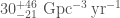 , and 3.
  . As expected, the first rate is nestled between the other two.
 , and that the less massive black hole has a mass uniformly distributed in mass ratio, down to a minimum black hole mass of
  . This has significant uncertainty, so we can’t say too much yet. This is a slightly steeper slope than used for the power-law rate (although entirely consistent with it), which would nudge the rates a little lower. The slope does fit in with fits to the distribution of masses in X-ray binaries. I’m excited to see how O2 will change our understanding of the distribution.
 at a frequency of 25 Hz to
  . This might be measurable after a few years at design sensitivity.
 . The median should really round to
  as to three significant figures it is
  . This really confused everyone though, as with rounding you’d have a binary with components of masses
  and
and  . Rounding is a pain! Fortunately,
  .
.

 and for some reason we’ve copied them. The second most significant event (around
  ) is LVT151012. Fig. 7 from the


 is converted into the measured signal


