Gravitational waves and gravitational lensing are two predictions of general relativity. Gravitational waves are produced whenever masses accelerate. Gravitational lensing is produced by anything with mass. Gravitational lensing can magnify images, making it easier to spot far away things. In theory, gravitational waves can be lensed too. In this paper, we looked for evidence that GW170814 might have been lensed. (We didn’t find any, but this was my first foray into traditional astronomy).
The lensing of gravitational waves
Strong gravitational lensing magnifies a signal. A gravitational wave which has been lensed would therefore have a larger amplitude than if it had not been lensed. We infer the distance to the source of a gravitational wave from the amplitude. If we didn’t know a signal was lensed, we’d therefore think the source is much closer than it really is.
The shape of the gravitational wave encodes the properties of the source. This information is what lets us infer parameters. The example signal is GW150914 (which is fairly similar to GW170814). I made this explainer with Ban Farr and Nutsinee Kijbunchoo for the LIGO Magazine.
Mismeasuring the distance to a gravitational wave has important consequences for understanding their sources. As the gravitational wave travels across the expanding Universe, it gets stretched (redshifted) so by the time it arrives at our detectors it has a longer wavelength (and shorter frequency). If we assume that a signal came from a closer source, we’ll underestimate the amount of stretching the signal has undergone, and won’t fully correct for it. This means we’ll overestimate the masses when we infer them from the signal.
This possibility got a few people thinking when we announced our first detection, as GW150914 was heavier than previously observed black holes. Could we be seeing lensed gravitational waves?
Such strongly lensed gravitational waves should be multiply imaged. We should be able to see multiple copies of the same signal which have taken different paths from the source and then are bent by the gravity of the lens to reach us at different times. The delay time between images depends on the mass of the lens, with bigger lensing having longer delays. For galaxy clusters, it can be years.
The idea
Some of my former Birmingham colleagues who study gravitational lensing, were thinking about the possibility of having multiply imaged gravitational waves. I pointed out how difficult these would be to identify. They would come from the same part of the sky, and would have the same source parameters. However, since our uncertainties are so large for gravitational wave observations, I thought it would be tough to convince yourself that you’d seen the same signal twice [bonus note]. Lensing is expected to be rare [bonus note], so would you put your money on two signals (possibly years apart) being the same, or there just happening to be two similar systems somewhere in this huge patch of the sky?
However, if there were an optical counterpart to the merger, it would be much easier to tell that it was lensed. Since we know the location of galaxy clusters which could strongly lens a signal, we can target searches looking for counterparts at these clusters. The odds of finding anything are slim, but since this doesn’t take too much telescope time to look it’s still a gamble worth taking, as the potential pay-off would be huge.
Somehow [bonus note], I got involved in observing proposals to look for strongly lensed. We got everything in place for the last month of O2. It was just one month, so I wasn’t anticipating there being that much to do. I was very wrong.
GW170814
For GW170814 there were a couple of galaxy clusters which could serve as being strong gravitational lenses. Abell 3084 started off as the more probably, but as the sky localization for GW170814 was refined, SMACS J0304.3−4401 looked like the better bet.
Sky localization for GW170814 and the galaxy clusters Abell 3084 (filled circle), and SMACS J0304.3−4401 (open). The left plot shows the low-latency Bayestar localization (LIGO only dotted, LIGO and Virgo solid), and the right shows the refined LALInference sky maps (solid from GCN 21493, which we used for our observations, and dotted from GWTC-1). The dashed lines shows the Galactic plane. Figure 1 of Smith et al. (2019).
That’s right, absolutely nothing! [bonus note] That’s not actually too surprising. GW170814‘s source was identified as a binary black hole—assuming no lensing, its source binary had masses around 25 and 30 solar masses. We don’t expect significant electromagnetic emission from a binary black hole merger (which would make it a big discovery if found, but that is a long shot). If there source were lensed, we would have overestimated the source masses, but to get the source into the neutron star mass range would take a ridiculous amount of lensing. However, the important point is that we have demonstrated that such a search for strong lensed images is possible!
The future
In O3 [bonus notebonus note], the team has been targeting lower mass systems, where a neutron star may get mislabelled as a black hole by mistake due to a moderate amount of lensing. A false identification here could confuse our understanding of the minimum mass of a black hole, and also mean that we miss all sorts of lovely multimessenger observations, so this seems like a good plan to me.
It is possible to do a statistical analysis to calculate the probability of two signals being lensed images of each. The best attempt I’ve seen at this is Hannuksela et al. (2019). They do a nice study considering lensing by galaxies (and find nothing conclusive).
Biasing merger rates
If we included lensed events in our calculations of the merger rate density (the rate of mergers per unit volume of space), without correcting for them being lensed, we would overestimate the merger rate density. We’d assume that all our mergers came from a smaller volume of space than they actually did, as we wouldn’t know that the lensed events are being seen from further away. As long as the fraction of lensed events is small, this shouldn’t be a big problem, so we’re probably safe not to worry about it.
Slippery slope
What actually happened was my then boss, Alberto Vecchio, asked me to do some calculations based upon the sky maps for our detections in O1 as they’d only take me 5 minutes. Obviously, there were then more calculations, advice about gravitational wave alerts, feedback on observing proposals… and eventually I thought that if I’d put in this much time I might as well get a paper to show for it.
It was interesting to see how electromagnetic observing works, but I’m not sure I’d do it again.
Upper limits
Following tradition, when we don’t make a detection, we can set an upper limit on what could be there. In this case, we conclude that there is nothing to see down to an i-band magnitude of 25. This is pretty faint, about 40 million times fainter than something you could see with the naked eye (translating to visibly light). We can set such a good upper limit (compared to other follow-up efforts) as we only needed to point the telescopes at a small patch of sky around the galaxy clusters, and so we could leave them staring for a relatively long time.
O3 lensing hype
In O3, two gravitational wave candidates (S190828j and S190828l) were found just 21 minutes apart—this, for reasons I don’t entirely understand, led to much speculation that they were multiple images of a gravitationally lensed source. For a comprehensive debunking, follow this Twitter thread.
On 4 January 2017, Advanced LIGO made a new detection of gravitational waves. The signal, which we call GW170104 [bonus note], came from the coalescence of two black holes, which inspiralled together (making that characteristic chirp) and then merged to form a single black hole.
On 4 January 2017, I was just getting up off the sofa when my phone buzzed. My new year’s resolution was to go for a walk every day, and I wanted to make use of the little available sunlight. However, my phone informed me that PyCBC (one or our search algorithms for signals from coalescing binaries) had identified an interesting event. I sat back down. I was on the rota to analyse interesting signals to infer their properties, and I was pretty sure that people would be eager to see results. They were. I didn’t leave the sofa for the rest of the day, bringing my new year’s resolution to a premature end.
Since 4 January, my time has been dominated by working on GW170104 (you might have noticed a lack of blog posts). Below I’ll share some of my war stories from life on the front line of gravitational-wave astronomy, and then go through some of the science we’ve learnt. (Feel free to skip straight to the science, recounting the story was more therapy for me).
Time–frequency plots for GW170104 as measured by Hanford (top) and Livingston (bottom). The signal is clearly visible as the upward sweeping chirp. The loudest frequency is something between E3 and G♯3 on a piano, and it tails off somewhere between D♯4/E♭4 and F♯4/G♭4. Part of Fig. 1 of the GW170104 Discovery Paper.
The story
In the second observing run, the Parameter Estimation group have divided up responsibility for analysing signals into two week shifts. For each rota shift, there is an expert and a rookie. I had assumed that the first slot of 2017 would be a quiet time. The detectors were offline over the holidays, due back online on 4 January, but the instrumentalists would probably find some extra tinkering they’d want to do, so it’d probably slip a day, and then the weather would be bad, so we’d probably not collect much data anyway… I was wrong. Very wrong. The detectors came back online on time, and there was a beautifully clean detection on day one.
My partner for the rota was Aaron Zimmerman. 4 January was his first day running parameter estimation on live signals. I think I would’ve run and hidden underneath my duvet in his case (I almost did anyway, and I lived through the madness of our first detection GW150914), but he rose to the occasion. We had first results after just a few hours, and managed to send out a preliminary sky localization to our astronomer partners on 6 January. I think this was especially impressive as there were some difficulties with the initial calibration of the data. This isn’t a problem for the detection pipelines, but does impact the parameters which we infer, particularly the sky location. The Calibration group worked quickly, and produced two updates to the calibration. We therefore had three different sets of results (one per calibration) by 6 January [bonus note]!
Producing the final results for the paper was slightly more relaxed. Aaron and I conscripted volunteers to help run all the various permutations of the analysis we wanted to double-check our results [bonus note].
Recovered gravitational waveforms from analysis of GW170104. The broader orange band shows our estimate for the waveform without assuming a particular source (wavelet). The narrow blue bands show results if we assume it is a binary black hole (BBH) as predicted by general relativity. The two match nicely, showing no evidence for any extra features not included in the binary black hole models. Figure 4 of the GW170104 Discovery Paper.
I started working on GW170104 through my parameter estimation duties, and continued with paper writing.
Ahead of the second observing run, we decided to assemble a team to rapidly write up any interesting binary detections, and I was recruited for this (I think partially because I’m not too bad at writing and partially because I was in the office next to John Veitch, one of the chairs of the Compact Binary Coalescence group,so he can come and check that I wasn’t just goofing off eating doughnuts). We soon decided that we should write a paper about GW170104, and you can decide whether or not we succeeded in doing this rapidly…
Being on the paper writing team has given me huge respect for the teams who led the GW150914 and GW151226 papers. It is undoubtedly one of the most difficult things I’ve ever done. It is extremely hard to absorb negative remarks about your work continuously for months [bonus note]—of course people don’t normally send comments about things that they like, but that doesn’t cheer you up when you’re staring at an inbox full of problems that need fixing. Getting a collaboration of 1000 people to agree on a paper is like herding cats while being a small duckling.
On of the first challenges for the paper writing team was deciding what was interesting about GW170104. It was another binary black hole coalescence—aren’t people getting bored of them by now? The signal was quieter than GW150914, so it wasn’t as remarkable. However, its properties were broadly similar. It was suggested that perhaps we should title the paper “GW170104: The most boring gravitational-wave detection”.
One potentially interesting aspect was that GW170104 probably comes from greater distance than GW150914 or GW151226 (but perhaps not LVT151012) [bonus note]. This might make it a good candidate for testing for dispersion of gravitational waves.
Dispersion occurs when different frequencies of gravitational waves travel at different speeds. A similar thing happens for light when travelling through some materials, which leads to prisms splitting light into a spectrum (and hence the creation of Pink Floyd album covers). Gravitational waves don’t suffered dispersion in general relativity, but do in some modified theories of gravity.
It should be easier to spot dispersion in signals which have travelled a greater distance, as the different frequencies have had more time to separate out. Hence, GW170104 looks pretty exciting. However, being further away also makes the signal quieter, and so there is more uncertainty in measurements and it is more difficult to tell if there is any dispersion. Dispersion is also easier to spot if you have a larger spread of frequencies, as then there can be more spreading between the highest and lowest frequencies. When you throw distance, loudness and frequency range into the mix, GW170104 doesn’t always come out on top, depending upon the particular model for dispersion: sometimes GW150914’s loudness wins, other times GW151226’s broader frequency range wins. GW170104 isn’t too special here either.
Even though GW170104 didn’t look too exciting, we started work on a paper, thinking that we would just have a short letter describing our observations. The Compact Binary Coalescence group decided that we only wanted a single paper, and we wouldn’t bother with companion papers as we did for GW150914. As we started work, and dug further into our results, we realised that actually there was rather a lot that we could say.
I guess the moral of the story is that even though you might be overshadowed by the achievements of your siblings, it doesn’t mean that you’re not awesome. There might not be one outstanding feature of GW170104, but there are lots of little things that make it interesting. We are still at the beginning of understanding the properties of binary black holes, and each new detection adds a little more to our picture.
I think GW170104 is rather neat, and I hope you do too.
As we delved into the details of our results, we realised there was actually a lot of things that we could say about GW170104, especially when considered with our previous observations. We ended up having to move some of the technical details and results to Supplemental Material. With hindsight, perhaps it would have been better to have a companion paper or two. However, I rather like how packed with science this paper is.
The paper, which Physical Review Letters have kindly accommodated, despite its length, might not be as polished a classic as the GW150914 Discovery Paper, but I think they are trying to do different things. I rarely ever refer to the GW150914 Discovery Paper for results (more commonly I use it for references), whereas I think I’ll open up the GW170104 Discovery Paper frequently to look up numbers.
Although perhaps not right away, I’d quite like some time off first. The weather’s much better now, perfect for walking…
Advanced LIGO’s first observing run was hugely successful. Running from 12 September 2015 until 19 January 2016, there were two clear gravitational-wave detections, GW1501914 and GW151226, as well as a less certain candidate signal LVT151012. All three (assuming that they are astrophysical signals) correspond to the coalescence of binary black holes.
The second observing run started 30 November 2016. Following the first observing run’s detections, we expected more binary black hole detections. On 4 January, after we had collected almost 6 days’ worth of coincident data from the two LIGO instruments [bonus note], there was a detection.
The searches
The signal was first spotted by an online analysis. Our offline analysis of the data (using refined calibration and extra information about data quality) showed that the signal, GW170104, is highly significant. For both GstLAL and PyCBC, search algorithms which use templates to search for binary signals, the false alarm rate is estimated to be about 1 per 70,000 years.
The signal is also found in unmodelled (burst) searches, which look for generic, short gravitational wave signals. Since these are looking for more general signals than just binary coalescences, the significance associated with GW170104 isn’t as great, and coherent WaveBurst estimates a false alarm rate of 1 per 20,000 years. This is still pretty good! Reconstructions of the waveform from unmodelled analyses also match the form expected for binary black hole signals.
The search false alarm rates are the rate at which you’d expect something this signal-like (or more signal-like) due to random chance, if you data only contained noise and no signals. Using our knowledge of the search pipelines, and folding in some assumptions about the properties of binary black holes, we can calculate a probability that GW170104 is a real astrophysical signal. This comes out to be greater than .
The source
As for the previous gravitational wave detections, GW170104 comes from a binary black hole coalescence. The initial black holes were and (where is the mass of our Sun), and the final black hole was . The quoted values are the median values and the error bars denote the central 90% probable range. The plot below shows the probability distribution for the masses; GW170104 neatly nestles in amongst the other events.
Estimated masses for the two black holes in the binary . The two-dimensional shows the probability distribution for GW170104 as well as 50% and 90% contours for all events. The one-dimensional plot shows results using different waveform models. The dotted lines mark the edge of our 90% probability intervals. Figure 2 of the GW170104 Discovery Paper.
GW150914 was the first time that we had observed stellar-mass black holes with masses greater than around . GW170104 has similar masses, showing that our first detection was not a fluke, but there really is a population of black holes with masses stretching up into this range.
Black holes have two important properties: mass and spin. We have good measurements on the masses of the two initial black holes, but not the spins. The sensitivity of the form of the gravitational wave to spins can be described by two effective spin parameters, which are mass-weighted combinations of the individual spins.
The effective inspiral spin parameter qualifies the impact of the spins on the rate of inspiral, and where the binary plunges together to merge. It ranges from +1, meaning both black holes are spinning as fast as possible and rotate in the same direction as the orbital motion, to −1, both black holes spinning as fast as possible but in the opposite direction to the way that the binary is orbiting. A value of 0 for could mean that the black holes are not spinning, that their rotation axes are in the orbital plane (instead of aligned with the orbital angular momentum), or that one black hole is aligned with the orbital motion and the other is antialigned, so that their effects cancel out.
The effective precession spin parameter qualifies the amount of precession, the way that the orbital plane and black hole spins wobble when they are not aligned. It is 0 for no precession, and 1 for maximal precession.
We can place some constraints on , but can say nothing about . The inferred value of the effective inspiral spin parameter is . Therefore, we disfavour large spins aligned with the orbital angular momentum, but are consistent with small aligned spins, misaligned spins, or spins antialigned with the angular momentum. The value is similar to that for GW150914, which also had a near-zero, but slightly negative of .
Estimated effective inspiral spin parameter and effective precession spin parameter. The two-dimensional shows the probability distribution for GW170104 as well as 50% and 90% contours. The one-dimensional plot shows results using different waveform models, as well as the prior probability distribution. The dotted lines mark the edge of our 90% probability intervals. We learn basically nothing about precession. Part of Figure 3 of the GW170104 Discovery Paper.
Converting the information about , the lack of information about , and our measurement of the ratio of the two black hole masses, into probability distributions for the component spins gives the plots below [bonus note]. We disfavour (but don’t exclude) spins aligned with the orbital angular momentum, but can’t say much else.
Estimated orientation and magnitude of the two component spins. The distribution for the more massive black hole is on the left, and for the smaller black hole on the right. The probability is binned into areas which have uniform prior probabilities, so if we had learnt nothing, the plot would be uniform. Part of Figure 3 of the GW170104 Discovery Paper.
One of the comments we had on a draft of the paper was that we weren’t making any definite statements about the spins—we would have if we could, but we can’t for GW170104, at least for the spins of the two inspiralling black holes. We can be more definite about the spin of the final black hole. If two similar mass black holes spiral together, the angular momentum from the orbit is enough to give a spin of around . The spins of the component black holes are less significant, and can make it a bit higher of lower. We infer a final spin of ; there is a tail of lower spin values on account of the possibility that the two component black holes could be roughly antialigned with the orbital angular momentum.
Estimated mass and spin for the final black hole. The two-dimensional shows the probability distribution for GW170104 as well as 50% and 90% contours. The one-dimensional plot shows results using different waveform models. The dotted lines mark the edge of our 90% probability intervals. Figure 6 of the GW170104 Supplemental Material (Figure 11 of the arXiv version).
If you’re interested in parameter describing GW170104, make sure to check out the big table in the Supplemental Material. I am a fan of tables [bonus note].
Merger rates
Adding the first 11 days of coincident data from the second observing run (including the detection of GW170104) to the results from the first observing run, we find merger rates consistent with those from the first observing run.
To calculate the merger rates, we need to assume a distribution of black hole masses, and we use two simple models. One uses a power law distribution for the primary (larger) black hole and a uniform distribution for the mass ratio; the other uses a distribution uniform in the logarithm of the masses (both primary and secondary). The true distribution should lie somewhere between the two. The power law rate density has been updated from to , and the uniform in log rate density goes from to . The median values stay about the same, but the additional data have shrunk the uncertainties a little.
Astrophysics
The discoveries from the first observing run showed that binary black holes exist and merge. The question is now how exactly they form? There are several suggested channels, and it could be there is actually a mixture of different formation mechanisms in action. It will probably require a large number of detections before we can make confident statements about the the probable formation mechanisms; GW170104 is another step towards that goal.
There are two main predicted channels of binary formation:
Isolated binary evolution, where a binary star system lives its life together with both stars collapsing to black holes at the end. To get the black holes close enough to merge, it is usually assumed that the stars go through a common envelope phase, where one star puffs up so that the gravity of its companion can steal enough material that they lie in a shared envelope. The drag from orbiting inside this then shrinks the orbit.
Dynamical evolution where black holes form in dense clusters and a binary is created by dynamical interactions between black holes (or stars) which get close enough to each other.
It’s a little artificial to separate the two, as there’s not really such a thing as an isolated binary: most stars form in clusters, even if they’re not particularly large. There are a variety of different modifications to the two main channels, such as having a third companion which drives the inner binary to merge, embedding the binary is a dense disc (as found in galactic centres), or dynamically assembling primordial black holes (formed by density perturbations in the early universe) instead of black holes formed through stellar collapse.
All the channels can predict black holes around the masses of GW170104 (which is not surprising given that they are similar to the masses of GW150914).
The updated rates are broadly consistent with most channels too. The tightening of the uncertainty of the rates means that the lower bound is now a little higher. This means some of the channels are now in tension with the inferred rates. Some of the more exotic channels—requiring a third companion (Silsbee & Tremain 2017; Antonini, Toonen & Hamers 2017) or embedded in a dense disc (Bartos et al. 2016; Stone, Metzger & Haiman 2016; Antonini & Rasio 2016)—can’t explain the full rate, but I don’t think it was ever expected that they could, they are bonus formation mechanisms. However, some of the dynamical models are also now looking like they could predict a rate that is a bit low (Rodriguez et al. 2016; Mapelli 2016; Askar et al. 2017; Park et al. 2017). Assuming that this result holds, I think this may mean that some of the model parameters need tweaking (there are more optimistic predictions for the merger rates from clusters which are still perfectly consistent), that this channel doesn’t contribute all the merging binaries, or both.
The spins might help us understand formation mechanisms. Traditionally, it has been assumed that isolated binary evolution gives spins aligned with the orbital angular momentum. The progenitor stars were probably more or less aligned with the orbital angular momentum, and tides, mass transfer and drag from the common envelope would serve to realign spins if they became misaligned. Rodriguez et al. (2016) gives a great discussion of this. Dynamically formed binaries have no correlation between spin directions, and so we would expect an isotropic distribution of spins. Hence it sounds quite simple: misaligned spins indicates dynamical formation (although we can’t tell if the black holes are primordial or stellar), and aligned spins indicates isolated binary evolution. The difficulty is the traditional assumption for isolated binary evolution potentially ignores a number of effects which could be important. When a star collapses down to a black hole, there may be a supernova explosion. There is an explosion of matter and neutrinos and these can give the black hole a kick. The kick could change the orbital plane, and so misalign the spin. Even if the kick is not that big, if it is off-centre, it could torque the black hole, causing it to rotate and so misalign the spin that way. There is some evidence that this can happen with neutron stars, as one of the pulsars in the double pulsar system shows signs of this. There could also be some instability that changes the angular momentum during the collapse of the star, possibly with different layers rotating in different ways [bonus note]. The spin of the black hole would then depend on how many layers get swallowed. This is an area of research that needs to be investigated further, and I hope the prospect of gravitational wave measurements spurs this on.
For GW170104, we know the spins are not large and aligned with the orbital angular momentum. This might argue against one variation of isolated binary evolution, chemically homogeneous evolution, where the progenitor stars are tidally locked (and so rotate aligned with the orbital angular momentum and each other). Since the stars are rapidly spinning and aligned, you would expect the final black holes to be too, if the stars completely collapse down as is usually assumed. If the stars don’t completely collapse down though, it might still be possible that GW170104 fits with this model. Aside from this, GW170104 is consistent with all the other channels.
Estimated effective inspiral spin parameter for all events. To indicate how much (or little) we’ve learnt, the prior probability distribution for GW170104 is shown (the other priors are similar).All of the events have at 90% probability. Figure 5 of the GW170104 Supplemental Material (Figure 10 of the arXiv version). This is one of my favourite plots [bonus note].
If we start looking at the population of events, we do start to notice something about the spins. All of the inferred values of are close to zero. Only GW151226 is inconsistent with zero. These values could be explained if spins are typically misaligned (with the orbital angular momentum or each other) or if the spins are typically small (or both). We know that black holes spins can be large from observations of X-ray binaries, so it would be odd if they are small for binary black holes. Therefore, we have a tentative hint that spins are misaligned. We can’t say why the spins are misaligned, but it is intriguing. With more observations, we’ll be able to confirm if it is the case that spins are typically misaligned, and be able to start pinning down the distribution of spin magnitudes and orientations (as well as the mass distribution). It will probably take a while to be able to say anything definite though, as we’ll probably need about 100 detections.
Tests of general relativity
As well as giving us an insight into the properties of black holes, gravitational waves are the perfect tools for testing general relativity. If there are any corrections to general relativity, you’d expect them to be most noticeable under the most extreme conditions, where gravity is strong and spacetime is rapidly changing, exactly as in a binary black hole coalescence.
We added extra terms to to the waveform and constrained their potential magnitudes. The results are pretty much identical to at the end of the first observing run (consistent with zero and hence general relativity). GW170104 doesn’t add much extra information, as GW150914 typically gives the best constraints on terms that modify the post-inspiral part of the waveform (as it is louder), while GW151226 gives the best constraint on the terms which modify the inspiral (as it has the longest inspiral).
We also chopped the waveform at a frequency around that of the innermost stable orbit of the remnant black hole, which is about where the transition from inspiral to merger and ringdown occurs, to check if the low frequency and high frequency portions of the waveform give consistent estimates for the final mass and spin. They do.
We have also done something slightly new, and tested for dispersion of gravitational waves. We did something similar for GW150914 by putting a limit on the mass of the graviton. Giving the graviton mass is one way of adding dispersion, but we consider other possible forms too. In all cases, results are consistent with there being no dispersion. While we haven’t discovered anything new, we can update our gravitational wave constraint on the graviton mass of less than .
The search for counterparts
We don’t discuss observations made by our astronomer partners in the paper (they are not our results). A number (28 at the time of submission) of observations were made, and I expect that there will be a series of papers detailing these coming soon. So far papers have appeared from:
AGILE—hard X-ray and gamma-ray follow-up. They didn’t find any gamma-ray signals, but did identify a weak potential X-ray signal occurring about 0.46 s before GW170104. It’s a little odd to have a signal this long before the merger. The team calculate a probability for such a coincident to happen by chance, and find quite a small probability, so it might be interesting to follow this up more (see the INTEGRAL results below), but it’s probably just a coincidence (especially considering how many people did follow-up the event).
ANTARES—a search for high-energy muon neutrinos. No counterparts are identified in a ±500 s window around GW170104, or over a ±3 month period.
AstroSat-CZTI and GROWTH—a collaboration of observations across a range of wavelengths. They don’t find any hard X-ray counterparts. They do follow up on a bright optical transient ATLASaeu, suggested as a counterpart to GW170104, and conclude that this is a likely counterpart of long, soft gamma-ray burst GRB 170105A.
ATLAS and Pan-STARRS—optical follow-up. They identified a bright optical transient 23 hours after GW170104, ATLAS17aeu. This could be a counterpart to GRB 170105A. It seems unlikely that there is any mechanism that could allow for a day’s delay between the gravitational wave emission and an electromagnetic signal. However, the team calculate a small probability (few percent) of finding such a coincidence in sky position and time, so perhaps it is worth pondering. I wouldn’t put any money on it without a distance estimate for the source: assuming it’s a normal afterglow to a gamma-ray burst, you’d expect it to be further away than GW170104’s source.
Borexino—a search for low-energy neutrinos. This paper also discusses GW150914 and GW151226. In all cases, the observed rate of neutrinos is consistent with the expected background.
Fermi (GBM and LAT)—gamma-ray follow-up. They covered an impressive fraction of the sky localization, but didn’t find anything.
INTEGRAL—gamma-ray and hard X-ray observations. No significant emission is found, which makes the event reported by AGILE unlikely to be a counterpart to GW170104, although they cannot completely rule it out.
The intermediate Palomar Transient Factory—an optical survey. While searching, they discovered iPTF17cw, a broad-line type Ic supernova which is unrelated to GW170104 but interesting as it an unusual find.
Mini-GWAC—a optical survey (the precursor to GWAC). This paper covers the whole of their O2 follow-up including GW170608.
NOvA—a search for neutrinos and cosmic rays over a wide range of energies. This paper covers all the events from O1 and O2, plus triggers from O3.
TOROS—optical follow-up. They identified no counterparts to GW170104 (although they did for GW170817).
If you are interested in what has been reported so far (no compelling counterpart candidates yet to my knowledge), there is an archive of GCN Circulars sent about GW170104.
Summary
Advanced LIGO has made its first detection of the second observing run. This is a further binary black hole coalescence. GW170104 has taught us that:
The discoveries of the first observing run were not a fluke. There really is a population of stellar mass black holes with masses above out there, and we can study them with gravitational waves.
Binary black hole spins may be typically misaligned or small. This is not certain yet, but it is certainly worth investigating potential mechanisms that could cause misalignment.
General relativity still works, even after considering our new tests.
If someone asks you to write a discovery paper, run. Run and do not look back.
If you’re looking for the most up-to-date results regarding GW170104, check out the O2 Catalogue Paper.
Bonus notes
Naming
Gravitational wave signals (at least the short ones, which are all that we have so far), are named by their detection date. GW170104 was discovered 2017 January 4. This isn’t too catchy, but is at least better than the ID number in our database of triggers (G268556) which is used in corresponding with our astronomer partners before we work out if the “GW” title is justified.
Previous detections have attracted nicknames, but none has stuck for GW170104. Archisman Ghosh suggested the Perihelion Event, as it was detected a few hours before the Earth reached its annual point closest to the Sun. I like this name, its rather poetic.
More recently, Alex Nitz realised that we should have called GW170104 the Enterprise-D Event, as the USS Enterprise’s registry number was NCC-1701. For those who like Star Trek: the Next Generation, I hope you have fun discussing whether GW170104 is the third or fourth (counting LVT151012) detection: “There are four detections!“
The 6 January sky map
I would like to thank the wi-fi of Chiltern Railways for their role in producing the preliminary sky map. I had arranged to visit London for the weekend (because my rota slot was likely to be quiet… ), and was frantically working on the way down to check results so they could be sent out. I’d also like to thank John Veitch for putting together the final map while I was stuck on the Underground.
Binary black hole waveforms
The parameter estimation analysis works by matching a template waveform to the data to see how well it matches. The results are therefore sensitive to your waveform model, and whether they include all the relevant bits of physics.
In the first observing run, we always used two different families of waveforms, to see what impact potential errors in the waveforms could have. The results we presented in discovery papers used two quick-to-calculate waveforms. These include the effects of the black holes’ spins in different ways
SEOBNRv2 has spins either aligned or antialigned with the orbital angular momentum. Therefore, there is no precession (wobbling of orientation, like that of a spinning top) of the system.
IMRPhenomPv2 includes an approximate description of precession, packaging up the most important information about precession into a single parameter.
For GW150914, we also performed a follow-up analysis using a much more expensive waveform SEOBNRv3 which more fully includes the effect of both spins on precession. These results weren’t ready at the time of the announcement, because the waveform is laborious to run.
For GW170104, there were discussions that using a spin-aligned waveform was old hat, and that we should really only use the two precessing models. Hence, we started on the endeavour of producing SEOBNRv3 results. Fortunately, the code has been sped up a little, although it is still not quick to run. I am extremely grateful to Scott Coughlin (one of the folks behind Gravity Spy), Andrea Taracchini and Stas Babak for taking charge of producing results in time for the paper, in what was a Herculean effort.
I spent a few sleepless nights, trying to calculate if the analysis was converging quickly enough to make our target submission deadline, but it did work out in the end. Still, don’t necessarily expect we’ll do this for a all future detections.
Since the waveforms have rather scary technical names, in the paper we refer to IMRPhenomPv2 as the effective precession model and SEOBNRv3 as the full precession model.
On distance
Distance measurements for gravitational wave sources have significant uncertainties. The distance is difficult to measure as it determined from the signal amplitude, but this is also influences by the binary’s inclination. A signal could either be close and edge on or far and face on-face off.
Estimated luminosity distance and binary inclination angle . The two-dimensional shows the probability distribution for GW170104 as well as 50% and 90% contours. The one-dimensional plot shows results using different waveform models. The dotted lines mark the edge of our 90% probability intervals. Figure 4 of the GW170104 Supplemental Material (Figure 9 of the arXiv version).
The uncertainty on the distance rather awkwardly means that we can’t definitely say that GW170104 came from a further source than GW150914 or GW151226, but it’s a reasonable bet. The 90% credible intervals on the distances are 250–570 Mpc for GW150194, 250–660 Mpc for GW151226, 490–1330 Mpc for GW170104 and 500–1500 Mpc for LVT151012.
Translating from a luminosity distance to a travel time (gravitational waves do travel at the speed of light, our tests of dispersion are consistent wit that!), the GW170104 black holes merged somewhere between 1.3 and 3.0 billion years ago. This is around the time that multicellular life first evolved on Earth, and means that black holes have been colliding longer than life on Earth has been reproducing sexually.
Time line
A first draft of the paper (version 2; version 1 was a copy-and-paste of the Boxing Day Discovery Paper) was circulated to the Compact Binary Coalescence and Burst groups for comments on 4 March. This was still a rough version, and we wanted to check that we had a good outline of the paper. The main feedback was that we should include more about the astrophysical side of things. I think the final paper has a better balance, possibly erring on the side of going into too much detail on some of the more subtle points (but I think that’s better than glossing over them).
A first proper draft (version 3) was released to the entire Collaboration on 12 March in the middle of our Collaboration meeting in Pasadena. We gave an oral presentation the next day (I doubt many people had read the paper by then). Collaboration papers are usually allowed two weeks for people to comment, and we followed the same procedure here. That was not a fun time, as there was a constant trickle of comments. I remember waking up each morning and trying to guess how many emails would be in my inbox–I normally low-balled this.
I wasn’t too happy with version 3, it was still rather rough. The members of the Paper Writing Team had been furiously working on our individual tasks, but hadn’t had time to look at the whole. I was much happier with the next draft (version 4). It took some work to get this together, following up on all the comments and trying to address concerns was a challenge. It was especially difficult as we got a series of private comments, and trying to find a consensus probably made us look like the bad guys on all sides. We released version 4 on 14 April for a week of comments.
The next step was approval by the LIGO and Virgo executive bodies on 24 April. We prepared version 5 for this. By this point, I had lost track of which sentences I had written, which I had merely typed, and which were from other people completely. There were a few minor changes, mostly adding technical caveats to keep everyone happy (although they do rather complicate the flow of the text).
The paper was circulated to the Collaboration for a final week of comments on 26 April. Most comments now were about typos and presentation. However, some people will continue to make the same comment every time, regardless of how many times you explain why you are doing something different. The end was in sight!
The paper was submitted to Physical Review Letters on 9 May. I was hoping that the referees would take a while, but the reports were waiting in my inbox on Monday morning.
The referee reports weren’t too bad. Referee A had some general comments, Referee B had some good and detailed comments on the astrophysics, and Referee C gave the paper a thorough reading and had some good suggestions for clarifying the text. By this point, I have been staring at the paper so long that some outside perspective was welcome. I was hoping that we’d have a more thorough review of the testing general relativity results, but we had Bob Wald as one of our Collaboration Paper reviewers (the analysis, results and paper are all reviewed internally), so I think we had already been held to a high standard, and there wasn’t much left to say.
We put together responses to the reports. There were surprisingly few comments from the Collaboration at this point. I guess that everyone was getting tired. The paper was resubmitted and accepted on 20 May.
One of the suggestions of Referee A was to include some plots showing the results of the searches. People weren’t too keen on showing these initially, but after much badgering they were convinced, and it was decided to put these plots in the Supplemental Material which wouldn’t delay the paper as long as we got the material submitted by 26 May. This seemed like plenty of time, but it turned out to be rather frantic at the end (although not due to the new plots). The video below is an accurate representation of us trying to submit the final version.
I have an email which contains the line “Many Bothans died to bring us this information” from 1 hour and 18 minutes before the final deadline.
After this, things were looking pretty good. We had returned the proofs of the main paper (I had a fun evening double checking the author list. Yes, all of them). We were now on version 11 of the paper.
Of course, there’s always one last thing. On 31 May, the evening before publication, Salvo Vitale spotted a typo. Nothing serious, but annoying. The team at Physical Review Letters were fantastic, and took care of it immediately!
There’ll still be one more typo, there always is…
Looking back, it is clear that the principal bottle-neck in publishing the results is getting the Collaboration to converge on the paper. I’m not sure how we can overcome this… Actually, I have some ideas, but none that wouldn’t involve some form of doomsday device.
Detector status
The sensitivities of the LIGO Hanford and Livinston detectors are around the same as they were in the first observing run. After the success of the first observing run, the second observing run is the difficult follow up album. Livingston has got a little better, while Hanford is a little worse. This is because the Livingston team concentrate on improving low frequency sensitivity whereas the Hanford team focused on improving high frequency sensitivity. The Hanford team increased the laser power, but this introduces some new complications. The instruments are extremely complicated machines, and improving sensitivity is hard work.
The current plan is to have a long commissioning break after the end of this run. The low frequency tweaks from Livingston will be transferred to Hanford, and both sites will work on bringing down other sources of noise.
While the sensitivity hasn’t improved as much as we might have hoped, the calibration of the detectors has! In the first observing run, the calibration uncertainty for the first set of published results was about 10% in amplitude and 10 degrees in phase. Now, uncertainty is better than 5% in amplitude and 3 degrees in phase, and people are discussing getting this down further.
Spin evolution
As the binary inspirals, the orientation of the spins will evolve as they precess about. We always quote measurements of the spins at a point in the inspiral corresponding to a gravitational wave frequency of 20 Hz. This is most convenient for our analysis, but you can calculate the spins at other points. However, the resulting probability distributions are pretty similar at other frequencies. This is because the probability distributions are primarily determined by the combination of three things: (i) our prior assumption of a uniform distribution of spin orientations, (ii) our measurement of the effective inspiral spin, and (iii) our measurement of the mass ratio. A uniform distribution stays uniform as spins evolve, so this is unaffected, the effective inspiral spin is approximately conserved during inspiral, so this doesn’t change much, and the mass ratio is constant. The overall picture is therefore qualitatively similar at different moments during the inspiral.
Footnotes
I love footnotes. It was challenging for me to resist having any in the paper.
Gravity waves
It is possible that internal gravity waves (that is oscillations of the material making up the star, where the restoring force is gravity, not gravitational waves, which are ripples in spacetime), can transport angular momentum from the core of a star to its outer envelope, meaning that the two could rotate in different directions (Rogers, Lin & Lau 2012). I don’t think anyone has studied this yet for the progenitors of binary black holes, but it would be really cool if gravity waves set the properties of gravitational wave sources.
I really don’t want to proof read the paper which explains this though.
Colour scheme
For our plots, we use a consistent colour coding for our events. GW150914 is blue; LVT151012 is green; GW151226 is red–orange, and GW170104 is purple. The colour scheme is designed to be colour blind friendly (although adopting different line styles would perhaps be more distinguishable), and is implemented in Python in the Seaborn package as colorblind. Katerina Chatziioannou, who made most of the plots showing parameter estimation results is not a fan of the colour combinations, but put a lot of patient effort into polishing up the plots anyway.
The most recent, and most sensitive, all-sky search for continuous gravitational waves shows no signs of a detection. These signals from rotating neutron stars remain elusive. New data from the advanced detectors may change this, but we will have to wait a while to find out. This at least gives us time to try to figure out what to do with a detection, should one be made.
New years and new limits
The start of the new academic year is a good time to make resolutions—much better than wet and windy January. I’m trying to be tidier and neater in my organisation. Amid cleaning up my desk, which is covered in about an inch of papers, I uncovered this recent Collaboration paper, which I had lost track of.
The paper is the latest in the continuous stream of non-detections of continuous gravitational waves. These signals could come from rotating neutron stars which are deformed or excited in some way, and the hope that from such an observation we could learn something about the structure of neutron stars.
The search uses old data from initial LIGO’s sixth science run. Searches for continuous waves require lots of computational power, so they can take longer than even our analyses of binary neutron star coalescences. This is a semi-coherent search, like the recent search of the Orion spur—somewhere between an incoherent search, which looks for signal power of any form in the detectors, and a fully coherent search, which looks for signals which exactly match the way a template wave evolves [bonus note]. The big difference compared to the Orion spur search, is that this one looks at the entire sky. This makes it less sensitive in those narrow directions, but means we are not excluding the possibility of sources from other locations.
Artist’s impression of the local part of the Milky Way. The yellow cones mark the extent of the Orion Spur spotlight search, and the pink circle shows the equivalent sensitivity of this all-sky search. Green stars indicate known pulsars. Original image: NASA/JPL-Caltech/ESO/R. Hurt.
The search identified 16 outliers, but an examination of all of these showed they could be explained either as an injected signal or as detector noise. Since no signals were found, we can instead place some upper limits on the strength of signals.
The plot below translates the calculated upper limits (above which there would have been a ~75%–95% chance of us detected the signal) into the size of neutron star deformations. Each curve shows the limits on detectable signals at different distance, depending upon their frequency and the rate of change of their frequency. The dotted lines show limits on ellipticity , a measure of how bumpy the neutron star is. Larger deformations mean quicker changes of frequency and produce louder signals, therefore they can can be detected further away.
Range of the PowerFlux search for rotating neutron stars assuming that spin-down is entirely due to gravitational waves. The solid lines show the upper limits as a function of the gravitational-wave frequency and its rate of change; the dashed lines are the corresponding limits on ellipticity, and the dotted line marks the maximum searched spin-down. Figure 6 of Abbott et al. (2016).
Neutron stars are something like giant atomic nuclei. Figuring the properties of the strange matter that makes up neutron stars is an extremely difficult problem. We’ll never be able to recreate such exotic matter in the laboratory. Gravitational waves give us a rare means of gathering experimental data on how this matter behaves. However, exactly how we convert a measurement of a signal into constraints on the behaviour of the matter is still uncertain. I think that making a detection might only be the first step in understanding the sources of continuous gravitational waves.
arXiv:1605.03233 [gr-qc] Journal:Physical Review D; 94(4):042002(14); 2016
Other new academic year resolution: To attempt to grow a beard. Beard stroking helps you think, right?
Bonus note
The semi-coherent search
As the first step of this search, the PowerFlux algorithm looks for power that changes in frequency as expected for a rotating neutron star: it factors in Doppler shifting due to the motion of the Earth and a plausible spin down (slowing of the rotation) of the neutron star. As a follow up, the Loosely Coherent algorithm is used, which checks for signals which match short stretches of similar templates. Any candidates to make it through all stages of refinement are then examined in more detail. This search strategy is described in detail for the S5 all-sky search.
The LIGO Scientific Collaboration is busy analysing the data we’re currently taking with Advanced LIGO at the moment. However, the Collaboration is still publishing results from initial LIGO too. The most recent paper is a search for continuous waves—signals that are an almost constant hum throughout the observations. (I expect they’d be quite annoying for the detectors). Searching for continuous waves takes a lot of computing power (you can help by signing up for Einstein@Home), and is not particularly urgent since the sources don’t do much, hence it can take a while for results to appear.
Supernova remnants
Massive stars end their lives with an explosion, a supernova. Their core collapses down and their outer layers are blasted off. The aftermath of the explosion can be beautiful, with the thrown-off debris forming a bubble expanding out into the interstellar medium (the diffuse gas, plasma and dust between stars). This structure is known as a supernova remnant.
The youngest known supernova remnant, G1.9+0.3 (it’s just 150 years old), observed in X-ray and optical light. The ejected material forms a shock wave as it pushes the interstellar material out of the way. Credit: NASA/CXC/NCSU/DSS/Borkowski et al.
At the centre of the supernova remnant may be what is left following the collapse of the core of the star. Depending upon the mass of the star, this could be a black hole or a neutron star (or it could be nothing). We’re interested in the case it is a neutron star.
Neutron stars
Neutron stars are incredibly dense. One teaspoon’s worth would have about as much mass as 300 million elephants. Neutron stars are like giant atomic nuclei. We’re not sure how matter behaves in such extreme conditions as they are impossible to replicate here on Earth.
If a neutron star rotates rapidly (we know many do) and has an uneven or if there are waves in the the neutron star that moves lots of material around (like Rossby waves on Earth), then it can emit continuous gravitational waves. Measuring these gravitational waves would tell you about how bumpy the neutron star is or how big the waves are, and therefore something about what the neutron star is made from.
Neutron stars are most likely to emit loud gravitational waves when they are young. This is for two reasons. First, the supernova explosion is likely to give the neutron star a big whack, this could ruffle up its surface and set off lots of waves, giving rise to the sort of bumps and wobbles that emit gravitational waves. As the neutron star ages, things can quiet down, the neutron star relaxes, bumps smooth out and waves dissipate. This leaves us with smaller gravitational waves. Second, gravitational waves carry away energy, slowing the rotation of the neutron star. This also means that the signal gets quieter (and harder) to detect as the neutron star ages.
Since young neutron stars are the best potential sources, this study looked at nine young supernova remnants in the hopes of finding continuous gravitational waves. Searching for gravitational waves from particular sources is less computationally expensive than searching the entire sky. The search included Cassiopeia A, which had been previously searched in LIGO’s fifth science run, and G1.9+0.3, which is only 150 years old, as discovered by Dave Green. The positions of the searched supernova remnants are shown in the map of the Galaxy below.
The nine young supernova remnants searched for continuous gravitational waves. The yellow dot marks the position of the Solar System. The green markers show the supernova remnants, which are close to the Galactic plane. Two possible positions for Vela Jr (G266.2−1.2) were used, since we are uncertain of its distance. Original image: NASA/JPL-Caltech/ESO/R. Hurt.
Gravitational-wave limits
No gravitational waves were found. The search checks how well template waveforms match up with the data. We tested that this works by injecting some fake signals into the data. Since we didn’t detect anything, we can place upper limits on how loud any gravitational waves could be. These limits were double-checked by injecting some more fake signals at the limit, to see if we could detect them. We quoted 95% upper limits, that is where we expect that if a signal was present we could see it 95% of the time. The results actually have a small safety margin built in, so the injected signals were typically found 96%–97% of the time. In any case, we are fairly sure that there aren’t gravitational waves at or above the upper limits.
These upper limits are starting to tell us interesting things about the size of neutron-star bumps and waves. Hopefully, with data from Advanced LIGO and Advanced Virgo, we’ll actually be able to make a detection. Then we’ll not only be able to say that these bumps and waves are smaller than a particular size, but they are this size. Then we might be able to figure out the recipe for making the stuff of neutron stars (I think it might be more interesting than just flour and water).
The first observing run (O1) of Advanced LIGO is nearly here, and with it the prospect of the first direct detection of gravitational waves. That’s all wonderful and exciting (far more exciting than a custard cream or even a chocolate digestive), but there’s a lot to be done to get everything ready. Aside from remembering to vacuum the interferometer tubes and polish the mirrors, we need to see how the data analysis will work out. After all, having put so much effort into the detector, it would be shame if we couldn’t do any science with it!
Parameter estimation
Since joining the University of Birmingham team, I’ve been busy working on trying to figure out how well we can measure things using gravitational waves. I’ve been looking at binary neutron star systems. We expect binary neutron star mergers to be the main source of signals for Advanced LIGO. We’d like to estimate how massive the neutron stars are, how fast they’re spinning, how far away they are, and where in the sky they are. Just published is my first paper on how well we should be able to measure things. This took a lot of hard work from a lot of people, so I’m pleased it’s all done. I think I’ve earnt a celebratory biscuit. Or two.
When we see something that looks like it could be a gravitational wave, we run code to analyse the data and try to work out the properties of the signal. Working out some properties is a bit trickier than others. Sadly, we don’t have an infinite number of computers, so it means it can take a while to get results. Much longer than the time to eat a packet of Jaffa Cakes…
The fastest algorithm we have for binary neutron stars is BAYESTAR. This takes the same time as maybe eating one chocolate finger. Perhaps two, if you’re not worried about the possibility of choking. BAYESTAR is fast as it only estimates where the source is coming from. It doesn’t try to calculate a gravitational-wave signal and match it to the detector measurements, instead it just looks at numbers produced by the detection pipeline—the code that monitors the detectors and automatically flags whenever something interesting appears. As far as I can tell, you give BAYESTAR this information and a fresh cup of really hot tea, and it uses Bayes’ theorem to work out how likely it is that the signal came from each patch of the sky.
To work out further details, we need to know what a gravitational-wave signal looks like and then match this to the data. This is done using a different algorithm, which I’ll refer to as LALInference. (As names go, this isn’t as cool as SKYNET). This explores parameter space (hopping between different masses, distances, orientations, etc.), calculating waveforms and then working out how well they match the data, or rather how likely it is that we’d get just the right noise in the detector to make the waveform fit what we observed. We then use another liberal helping of Bayes’ theorem to work out how probable those particular parameter values are.
It’s rather difficult to work out the waveforms, but some our easier than others. One of the things that makes things trickier is adding in the spins of the neutron stars. If you made a batch of biscuits at the same time you started a LALInference run, they’d still be good by the time a non-spinning run finished. With a spinning run, the biscuits might not be quite so appetising—I generally prefer more chocolate than penicillin on my biscuits. We’re working on speeding things up (if only to prevent increased antibiotic resistance).
In this paper, we were interested in what you could work out quickly, while there’s still chance to catch any explosion that might accompany the merging of the neutron stars. We think that short gamma-ray bursts and kilonovae might be caused when neutron stars merge and collapse down to a black hole. (I find it mildly worrying that we don’t know what causes these massive explosions). To follow-up on a gravitational-wave detection, you need to be able to tell telescopes where to point to see something and manage this while there’s still something that’s worth seeing. This means that using spinning waveforms in LALInference is right out, we just use BAYESTAR and the non-spinning LALInference analysis.
What we did
To figure out what we could learn from binary neutron stars, we generated a large catalogue of fakes signals, and then ran the detection and parameter-estimation codes on this to see how they worked. This has been done before in The First Two Years of Electromagnetic Follow-Up with Advanced LIGO and Virgo which has a rather delicious astrobites write-up. Our paper is the sequel to this (and features most of the same cast). One of the differences is that The First Two Years assumed that the detectors were perfectly behaved and had lovely Gaussian noise. In this paper, we added in some glitches. We took some real data™ from initial LIGO’s sixth science run and stretched this so that it matches the sensitivity Advanced LIGO is expected to have in O1. This process is called recolouring [bonus note]. We now have fake signals hidden inside noise with realistic imperfections, and can treat it exactly as we would real data. We ran it through the detection pipeline, and anything which was flagged as probably being a signal (we used a false alarm rate of once per century), was analysed with the parameter-estimation codes. We looked at how well we could measure the sky location and distance of the source, and the masses of the neutron stars. It’s all good practice for O1, when we’ll be running this analysis on any detections.
What we found
The flavour of noise (recoloured or Gaussian) makes no difference to how well we can measure things on average.
Sky-localization in O1 isn’t great, typically hundreds of square degrees (the median 90% credible region is 632 deg2), for comparison, the Moon is about a fifth of a square degree. This’ll make things interesting for the people with telescopes.
Probability that of a gravitational-wave signal coming from different points on the sky. The darker the red, the higher the probability. The star indicates the true location. This is one of the worst localized events from our study for O1. You can find more maps in the data release (including 3D versions), this is Figure 6 of Berry et al. (2015).
BAYESTAR does just as well as LALInference, despite being about 2000 times faster.
Sky localization (the size of the patch of the sky that we’re 90% sure contains the source location) varies with the signal-to-noise ratio (how loud the signal is). The approximate best fit is , where is the 90% sky area and is the signal-to-noise ratio. The results for BAYESTAR and LALInference agree, as do the results with Gaussian and recoloured noise. This is Figure 9 of Berry et al. (2015).
We can’t measure the distance too well: the median 90% credible interval divided by the true distance (which gives something like twice the fractional error) is 0.85.
Because we don’t include the spins of the neutron stars, we introduce some error into our mass measurements. The chirp mass, a combination of the individual masses that we’re most sensitive to [bonus note], is still reliably measured (the median offset is 0.0026 of the mass of the Sun, which is tiny), but we’ll have to wait for the full spinning analysis for individual masses.
Fraction of events with difference between the mean estimated and true chirp mass smaller than a given value. There is an error because we are not including the effects of spin, but this is small. Again, the type of noise makes little difference. This is Figure 15 of Berry et al. (2015).
There’s still some work to be done before O1, as we need to finish up the analysis with waveforms that include spin. In the mean time, our results are all available online for anyone to play with.
The colour of noise: Noise is called white if it doesn’t have any frequency dependence. We made ours by taking some noise with initial LIGO’s frequency dependence (coloured noise), removing the frequency dependence (making it white), and then adding in the frequency dependence of Advanced LIGO (recolouring it).
The chirp mass: Gravitational waves from a binary system depend upon the masses of the components, we’ll call these and . The chirp mass is a combination these that we can measure really well, as it determines the most significant parts of the shape of the gravitational wave. It’s given by
.
We get lots of good information on the chirp mass, unfortunately, this isn’t too useful for turning back into the individual masses. For that we next extra information, for example the mass ratio . We can get this from less dominant parts of the waveform, but it’s not typically measured as precisely as the chirp mass, so we’re often left with big uncertainties.
A new paper from the LIGO Scientific Collaboration has snuck out. It was actually published back in March but I didn’t notice it, nearly risking my New Year’s resolution. This is another paper on continuous waves from rotating neutron stars, so it’s a little outside my area of expertise. However, there is an official science summary written by people who do know what they’re talking about.
The paper looks at detecting gravitational waves from a spinning neutron star. We didn’t find any. However, we have slightly improved our limit for how loud they need to be before we would have detected them, which is nice.
Neutron stars can rotate rapidly. They can be spun up if they accrete material from a disc orbiting them. If they neutron star has an asymmetry, if it has a little bump, as it rotates it emits gravitational waves. The gravitational waves carry away angular momentum, which should spin down the neutron star. This becomes more effective as the angular velocity increases. At some point you expect that the spin-up effect from accretion balances the spin-down effect of gravitational waves and you are left with a neutron star spinning at pretty constant velocity. We have some evidence that this might happen, as low-mass X-ray binaries seem to have their spins clustered in a small range of frequencies. Assuming we do have this balance, we are looking for a continuous gravitational wave with constant frequency, a rather dull humming.
Scorpius X-1 is the brightest X-ray source in the sky. It contains a neutron star, so it’s a good place to check for gravitational waves from neutron stars. In this case, we’re using data from initial LIGO’s fifth science run (4 November 2005–1 October 2007). This has been done before, but this paper implements some new techniques. I expect that the idea is to test things out ahead of getting data with Advanced LIGO.
Swift X-ray Telescope image of Scorpius X-1 and the X-ray nova J1745-26 (a stellar-mass black hole), along with the scale of moon, as they would appear in the field of view from Earth. Credit: NASA/Goddard Space Flight Center/S. Immler and H. Krimm.
A limit of 10 days’ worth of data is used, as this should be safely within the time taken for the rotational frequency to fluctuate by a noticeable amount due to variation in the amount of accretion. In human terms, that would be the time between lunch and dinner, where your energy levels change because of how much you’ve eaten. They picked data from 21–31 August 2007, as their favourite (it has the best noise performance over the frequency range of interest), and used two other segments to double-check their findings. We’d be able to use more data if we knew how the spin wandered with time.
We already know a lot about Scorpius X-1 from electromagnetic observations (like where it is and its orbital parameters). We don’t know its spin frequency, but we might have an idea about the orientation of its spin if this coincides with radio jets. The paper considers two cases: one where we don’t know anything about the spin orientation, and one where we use information from the jets. The results are similar in both cases.
As the neutron star orbits in its binary system, it moves back and forth which Doppler shifts the gravitational waves. This adds a little interest to the hum, spreading it out over a range of frequencies. The search looks for gravitational waves over this type of frequency range, which they refer to as sidebands.
There are a few events where it looks like there is something, but after carefully checking, these look like they are entirely consistent with noise. I guess this isn’t too surprising. Since they didn’t detect anything, they can only impose an upper limit. This is stronger than the previous upper limit, but only by a factor of about 1.4. This might not sound too great, but the previous analysis used a year of data, whereas this only used 10 days. This method therefore saves a lot on computational time.
The result of the paper is quite nice, but not too exciting. If it were a biscuit, it’d probably be a rich tea. It’s nice to have, but it’s not a custard cream.
Continuing with my New Year’s resolution to write a post on every published paper, the start of March see another full author list LIGO publication. Appearing in Classical & Quantum Gravity, the minimalistically titled Advanced LIGO is an instrumental paper. It appears a part of a special focus issue on advanced gravitational-wave detectors, and is happily free to read (good work there). This is The Paper™ for describing how the advanced detectors operate. I think it’s fair to say that my contribution to this paper is 0%.
LIGO stands for Laser Interferometer Gravitational-wave Observatory. As you might imagine, LIGO tries to observe gravitational waves by measuring them with a laser interferometer. (It won’t protect your fencing). Gravitational waves are tiny, tiny stretches and squeezes of space. To detect them we need to measure changes in length extremely accurately. I had assumed that Advanced LIGO will achieve this supreme sensitivity through some dark magic invoked by sacrificing the blood, sweat, tears and even coffee of many hundreds of PhD students upon the altar of science. However, this paper actually shows it’s just really, really, REALLY careful engineering. And giant frickin’ laser beams.
The paper goes through each aspect of the design of the LIGO detectors. It starts with details of the interferometer. LIGO uses giant lasers to measure distances extremely accurately. Lasers are bounced along two 3994.5 m arms and interfered to measure a change in length between the two. In spirit, it is a giant Michelson interferometer, but it has some cunning extra features. Each arm is a Fabry–Pérot etalon, which means that the laser is bounced up and down the arms many times to build up extra sensitivity to any change in length. There are various extra components to make sure that the laser beam is as stable as possible, all in all, there are rather a lot of mirrors, each of which is specially tweaked to make sure that some acronym is absolutely perfect.
Fig. 1 from Aasi et al. (2015), the Advanced LIGO optical configuration. All the acronyms have to be carefully placed in order for things to work. The laser beam starts from the left, passing through subsystems to make sure it’s stable. It is split in two to pass into the interferometer arms at the top and right of the diagram. The laser is bounced many times between the mirrors to build up sensitivity. The interference pattern is read out at the bottom. Normally, the light should interfere destructively, so the output is dark. A change to this indicates a change in length between the arms. That could be because of a passing gravitational wave.
The next section deals with all the various types of noise that affect the detector. It’s this noise that makes it such fun to look for the signals. To be honest, pretty much everything I know about the different types of noise I learnt from Space-Time Quest. This is a lovely educational game developed by people here at the University of Birmingham. In the game, you have to design the best gravitational-wave detector that you can for a given budget. There’s a lot of science that goes into working out how sensitive the detector is. It takes a bit of practice to get into it (remember to switch on the laser first), but it’s very easy to get competitive. We often use the game as part of outreach workshops, and we’ve had some school groups get quite invested in the high-score tables. My tip is that going underground doesn’t seem to be worth the money. Of course, if you happen to be reviewing the proposal to build the Einstein Telescope, you should completely ignore that, and just concentrate how cool the digging machine looks. Space-Time Quest shows how difficult it can be optimising sensitivity. There are trade-offs between different types of noise, and these have been carefully studied. What Space-Time Quest doesn’t show, is just how much work it takes to engineer a detector.
The fourth section is a massive shopping list of components needed to build Advanced LIGO. There are rather more options than in Space-Time Quest, but many are familiar, even if given less friendly names. If this section were the list of contents for some Ikea furniture, you would know that you’ve made a terrible life-choice; there’s no way you’re going to assemble this before Monday. Highlights include the 40 kg mirrors. I’m sure breaking one of those would incur more than seven years bad luck. For those of you playing along with Space-Time Quest at home, the mirrors are fused silica. Section 4.8.4 describes how to get the arms to lock, one of the key steps in commissioning the detectors. The section concludes with details of how to control such a complicated instrument, the key seems to be to have so many acronyms that there’s no space for any component to move in an unwanted way.
The paper closes with on outlook for the detector sensitivity. With such a complicated instrument it is impossible to be certain how things will go. However, things seem to have been going smoothly so far, so let’s hope that this continues. The current plan is:
2015 3 months observing at a binary neutron star (BNS) range of 40–80 Mpc.
2016–2017 6 months observing at a BNS range of 80–120 Mpc.
2017–2018 9 months observing at a BNS range of 120–170 Mpc.
2019 Achieve full sensitivity of a BNS range of 200 Mpc.
The BNS range is the distance at which a typical binary made up of two 1.4 solar mass neutrons stars could be detected when averaging over all orientations. If you have a perfectly aligned binary, you can detect it out to a further distance, the BNS horizon, which is about 2.26 times the BNS range. There are a couple of things to note from the plan. First, the initial observing run (O1 to the cool kids) is this year! The second is how much the range will extend before hitting design sensitivity. This should significantly increase the number of possible detections, as each doubling of the range corresponds to a volume change of a factor of eight. Coupling this with the increasing length of the observing runs should mean that the chance of a detection increases every year. It will be an exciting few years for Advanced LIGO.
I’ve been a member of the LIGO Scientific Collaboration for just over a year now. It turns out that designing, building and operating a network of gravitational-wave detectors is rather tricky, maybe even harder than completing Super Mario Bros. 3, so it takes a lot of work. There are over 900 collaboration members, all working on different aspects of the project. Since so much of the research is inter-related, certain papers (such as those that use data from the instruments) written by collaboration members have to include the name of everyone who works (at least half the time) on LIGO-related things. After a year in the collaboration, I have now levelled up to be included in the full author list (if there was an initiation ritual, I’ve suppressed the memory). This is weird: papers appear with my name on that I’ve not actually done any work for. It seems sort of like having to bring cake into your office on your birthday: you do have to share your (delicious) cupcakes with everyone else, but in return you get cake even when your birthday is nowhere near. Perhaps all those motivational posters where right about the value of teamwork? I do feel a little guilty about all the extra trees that will die because of people printing out these papers.
My New Year’s resolution was to write a post about every paper I have published. I am going to try to do the LIGO papers too. This should at least make sure that I actually read them all. There are official science summaries written by the people who did actually do the work, which may be better if you actually want an accurate explanation. My first collaboration paper is a joint publication of the LIGO and Virgo collaborations (even more sharing).
Searching for gravitational waves from pulsars
Neutron stars are formed from the cores of dead stars. When a star’s nuclear fuel starts to run out, their core collapses. The most massive form black holes, the lightest (like our Sun) form white dwarfs, and the ones in the middle form neutron stars. These are really dense, they have about the same mass as our entire Sun (perhaps twice the Sun’s mass), but are just a few kilometres across. Pulsars are a type of neutron star, they emit a beam of radiation that sweeps across the sky as they rotate, sort of like a light-house. If one of these beams hits the Earth, we see a radio pulse. The pulses come regularly, so you can work out how fast the pulsar is spinning (and do some other cool things too).
The mandatory cartoon of a pulsar that everyone uses. The top part shows the pulsar and its beams rotating, and the bottom part shows the signal measured on Earth. We not really sure where the beams come from, it’ll be something to do with magnetic fields. Credit: M. Kramer
Because pulsars rotate really quickly, if they have a little bump on their surface, they can emit (potentially detectable) gravitational waves. This paper searches for these signals from the Crab and Vela pulsars. We know where these pulsars are, and how quickly they are rotating, so it’s possible to do a targeted search for gravitational waves (only checking the data for signals that are close to what we expect). Importantly, some wiggle room in the frequency is allowed just in case different parts of the pulsar slosh around at slightly different rates and so the gravitational-wave frequency doesn’t perfectly match what we’d expect from the frequency of pulses; the search is done in a narrow band of frequencies around the expected one. The data used is from Virgo’s fourth science run (VSR4). That was taken back in 2011 (around the time that Captain America was released). The search technique is new (Astone et al., 2014), it’s the first one that incorporates this searching in a narrow band of frequencies; I think the point was to test their search technique on real data before the advanced detectors start producing new data.
Composite image of Hubble (red) optical observations and Chandra (blue) X-ray observations of the Crab pulsar. The pulsar has a mass of 1.4 solar masses and rotates every 30 ms. Credit: Hester et al.
The pulsars emit gravitational waves continuously, they just keep humming as they rotate. The frequency will slow gradually as the pulsar loses energy. As the Earth rotates, the humming gets louder and quieter because the sensitivity of gravitational-wave detectors depends upon where the source is in the sky. Putting this all together gives you a good template for what the signal should look like, and you can see how well it fits the data. It’s kind of like trying to find the right jigsaw piece by searching for the one that interlocks best with those around it. Of course, there is a lot of noise in our detectors, so it’s like if the jigsaw was actually made out of jelly: you could get many pieces to fit if you squeeze them the right way, but then people wouldn’t believe that you’ve actually found the right one. Some detection statistics (which I don’t particularly like, but probably give a sensible answer) are used to quantify how likely it is that they’ve found a piece that fits (that there is a signal). The whole pipeline is tested by analysing some injected signals (artificial signals made to see if things work made both by adding signals digitally to the data and by actually jiggling the mirrors of the interferometer). It seems to do OK here.
Turning to the actual data, they very carefully show that they don’t think they’ve detected anything for either Vela or Crab. Of course, all the cool kids don’t detect gravitational waves, so that’s not too surprising.
This paper doesn’t claim a detection of gravitational waves, but it doesn’t stink like Zoidberg.
Having not detected anything, you can place an upper limit of the amplitude of any waves that are emitted (because if they were larger, you would’ve detected them). This amplitude can then be compared with what’s expected from the spin-down limit: the amplitude that would be required to explain the slowing of the pulsar. We know how the pulsars are slowing, but not why; it could be because of energy being lost to magnetic fields (the energy for the beams has to come from somewhere), it could be through energy lost as gravitational waves, it could be because of some internal damping, it could all be gnomes. The spin-down limit assumes that it’s all because of gravitational waves, you couldn’t have bigger amplitude waves than this unless something else (that would have to be gnomes) was pumping energy into the pulsar to keep it spinning. The upper limit for the Vela pulsar is about the same as the spin-down limit, so we’ve not learnt anything new. For the Crab pulsar, the upper limit is about half the spin-down limit, which is something, but not really exciting. Hopefully, doing the same sort of searches with data from the advanced detectors will be more interesting.
In conclusion, the contents of this paper are well described by its title:
Narrow-band search: It uses a new search technique that is not restricted to the frequency assumed from timing pulses
of continuous gravitational-wave signals: It’s looking for signals from rotating neutron stars (that just keep going) and so are always in the data
from Crab and Vela pulsars: It considers two particular sources, so we know where in parameter space to look for signals
in Virgo VSR4 data: It uses real data, but from the first generation detectors, so it’s not surprising it doesn’t see anything
It’s probably less fun that eating a jigsaw-shaped jelly, but it might be more useful in the future.
Differing weights and differing measures—
the LORD detests them both. — Proverbs 20:10
As a New Year’s resolution, I thought I would try to write a post on each paper I have published. (I might try to go back and talk about my old papers too, but that might be a little too optimistic.) Handily, I have a paper that was published in Classical & Quantum Gravity on Thursday, so let’s get on with it, and hopefully 2015 will deliver those hoverboards soon.
This paper was written in collaboration with my old officemates, Chris Moore and Rob Cole, and originates from my time in Cambridge. We were having a weekly group meeting (surreptitiously eating cake—you’re not meant to eat in the new meeting rooms) and discussing what to do for the upcoming open afternoon. Posters are good as you can use them to decorate your office afterwards, so we decided on making one on gravitational-wave astronomy. Gravitational waves come in a range of frequencies, just like light (electromagnetic radiation). You can observe different systems with different frequencies, but you need different instruments to do so. For light, the range is from high frequency gamma rays (observed with satellites like Fermi) to low frequency radio waves (observed with telescopes like those at Jodrell Bank or Arecibo), with visible light (observed with Hubble or your own eyes) in the middle. Gravitational waves also have a spectrum, ground-based detectors like LIGO measure the higher frequencies, pulsar timing arrays measure the lower frequencies, and space-borne detectors like eLISA measure stuff in the middle. We wanted a picture that showed the range of each instrument and the sources they could detect, but we couldn’t find a good up-to-date one. Chris is not one to be put off by a challenge (especially if it’s a source of procrastination), so he decided to have a go at making one himself. How hard could it be? We never made that poster, but we did end up with a paper.
When talking about gravitational-wave detectors, you normally use a sensitivity curve. This shows how sensitive it is at a given frequency: you plot a graph with the sensitivity curve on, and then plot the spectrum of the source you’re interested in on the same graph. If your source is above the sensitivity curve, you can detect it (yay), but if it lies below it, then you can’t pick it out from the noise (boo). Making a plot with lots of sensitivity curves on sounds simple: you look up the details for lots of detectors, draw them together and add a few sources. However, there are lots of different conventions for how you actually measure sensitivity, and they’re frequently muddled up! We were rather confused by the whole thing, but eventually (after the open afternoon had flown by), we figured things out and made our picture. So we wouldn’t forget, we wrote up the different conventions, why you might want to use each, and how to convert between them; these notes became the paper. We also thought it would be handy to have a website where you could make your own plot, picking which detectors and sources you wanted to include. Rob also likes a challenge (especially if it’s a source of procrastination), so he set about making such a thing. I think it turned out rather well!
That’s the story of the paper. It explains different conventions for characterising gravitational-wave detectors and sources, and gives some examples. If you’d actually like to know some of the details, I’ll give a little explanation now, if not, just have a look at the pretty plots below (or, if looking for your own source of procrastination, have a go at Space Time Quest, a game where you try to build the most sensitive detector).
There are three common conventions in use for sensitivity-curve plots: the characteristic strain, the amplitude spectral density and the energy density.
You might wonder why we don’t just directly use the amplitude of the wave? Gravitational waves are a stretching and squashing of spacetime, so you can characterise how much they stretch and squeeze things and use that to describe the size of your waves. The sensitivity of your detector is then how much various sources of noise cause a similar wibbling. The amplitude of the wave is really, really small, so it’s difficult to detect, but if you were to consider observations over a time interval instead of just one moment, it’s easier to spot a signal: hints that there might be a signal add up until you’re certain that it’s there. The characteristic strain is a way of modifying the amplitude to take into account how we add up the signal. It’s especially handy, as if you make a log–log plot (such that the space between 1 and 10 is the same as between 10 and 100, etc.), then the area between the characteristic strain of your source and the detector sensitivity curve gives you a measure of the signal-to-noise ratio, a measure of how loud (how detectable) a signal is.
Gravitational-wave sensitivity-curve plot using characteristic strain. The area between the detector’s curve and the top of the box for a source indicates how loud that signal would be.
The characteristic strain is handy for quickly working out how loud a signal is, but it’s not directly related to anything we measure. The noise in a detector is usually described by its power spectral density or PSD. This tells you how much wibbling there is on average. Actually, it tells you the average amount of wibbling squared. The square root of the PSD is the amplitude spectral density or ASD. This gives a handy indication of the sensitivity of your detector, which is actually related to what you measure.
Gravitational-wave sensitivity-curve plot using the square root of the power spectral density (the amplitude spectral density).
The PSD is tied to the detector, but isn’t too relevant to the actual waves. An interesting property of the waves is how much energy they carry. We talk about this in terms of the energy density, the energy per unit volume. Cosmologists love this, and to make things easy for themselves, they like to divide energy densities by the amount that would make the Universe flat. (If you’ve ever wondered what astrophysicists mean when they say the Universe is about 70% dark energy and about 25% dark matter, they’re using these quantities). To make things even simpler, they like to multiply this quantity by something related to the Hubble constant (which measures the expansion rate of the Universe), as this means things don’t change if you tweak the numbers describing how the Universe evolves. What you’re left with is a quantity that is really convenient if you’re a cosmologist, but a pain for anyone else. It does have the advantage of making the pulsar timing arrays look more sensitive though.
Gravitational-wave sensitivity-curve plot using the energy density that cosmologists love. The proper name of the plotted quantity is the critical energy density per logarithmic frequency interval multiplied by the reduced Hubble constant squared. I prefer Bob.
We hope that the paper will be useful for people (like us), who can never remember what the conventions are (and why). There’s nothing new (in terms of results) in this paper, but I think it’s the first time all this material has been collected together in one place. If you ever need to make a poster about gravitational waves, I know where you can find a good picture.


 .
. and
and  (where
  is the mass of our Sun), and the final black hole was
  . The quoted values are the median values and the error bars denote the
 . The two-dimensional shows the probability distribution for GW170104 as well as 50% and 90% contours for all events. The one-dimensional plot shows results using different waveform models. The dotted lines mark the edge of our 90% probability intervals. Figure 2 of the
  . GW170104 has similar masses, showing that our first detection was not a fluke, but there really is a population of black holes with masses stretching up into this range.
 qualifies the impact of the spins on the rate of inspiral, and where the binary plunges together to merge. It ranges from +1, meaning both black holes are spinning as fast as possible and rotate in the same direction as the orbital motion, to −1, both black holes spinning as fast as possible but in the opposite direction to the way that the binary is orbiting. A value of 0 for
  qualifies the amount of precession, the way that the orbital plane and black hole
  . Therefore, we disfavour large spins aligned with the orbital angular momentum, but are consistent with small aligned spins, misaligned spins, or spins antialigned with the angular momentum. The value is similar to that for
  .
.

 . The spins of the component black holes are less significant, and can make it a bit higher of lower. We infer a final spin of
  ; there is a tail of lower spin values on account of the possibility that the two component black holes could be roughly antialigned with the orbital angular momentum.
 and spin
 for the final black hole. The two-dimensional shows the probability distribution for GW170104 as well as 50% and 90% contours. The one-dimensional plot shows results using different waveform models. The dotted lines mark the edge of our 90% probability intervals. Figure 6 of the GW170104 Supplemental Material (Figure 11 of the
  to
to  , and the uniform in log rate density goes from
  to
to  . The median values stay about the same, but the additional data have shrunk the uncertainties a little.
 at 90% probability. Figure 5 of the GW170104 Supplemental Material (Figure 10 of the
  .
.
 and binary inclination angle
  . The two-dimensional shows the probability distribution for GW170104 as well as 50% and 90% contours. The one-dimensional plot shows results using different waveform models. The dotted lines mark the edge of our 90% probability intervals. Figure 4 of the GW170104 Supplemental Material (Figure 9 of the
 , a measure of how bumpy the neutron star is. Larger deformations mean quicker changes of frequency and produce louder signals, therefore they can can be detected further away.


 , where
  is the 90% sky area and
  is the signal-to-noise ratio. The results for BAYESTAR and LALInference agree, as do the results with Gaussian and recoloured noise. This is Figure 9 of Berry et al. (
 and
and  . The chirp mass is a combination these that we can measure really well, as it determines the most significant parts of the shape of the gravitational wave. It’s given by
 .
. . We can get this from less dominant parts of the waveform, but it’s not typically measured as precisely as the chirp mass, so we’re often left with big uncertainties.


 that is really convenient if you’re a cosmologist, but a pain for anyone else. It does have the advantage of making the pulsar timing arrays look more sensitive though.

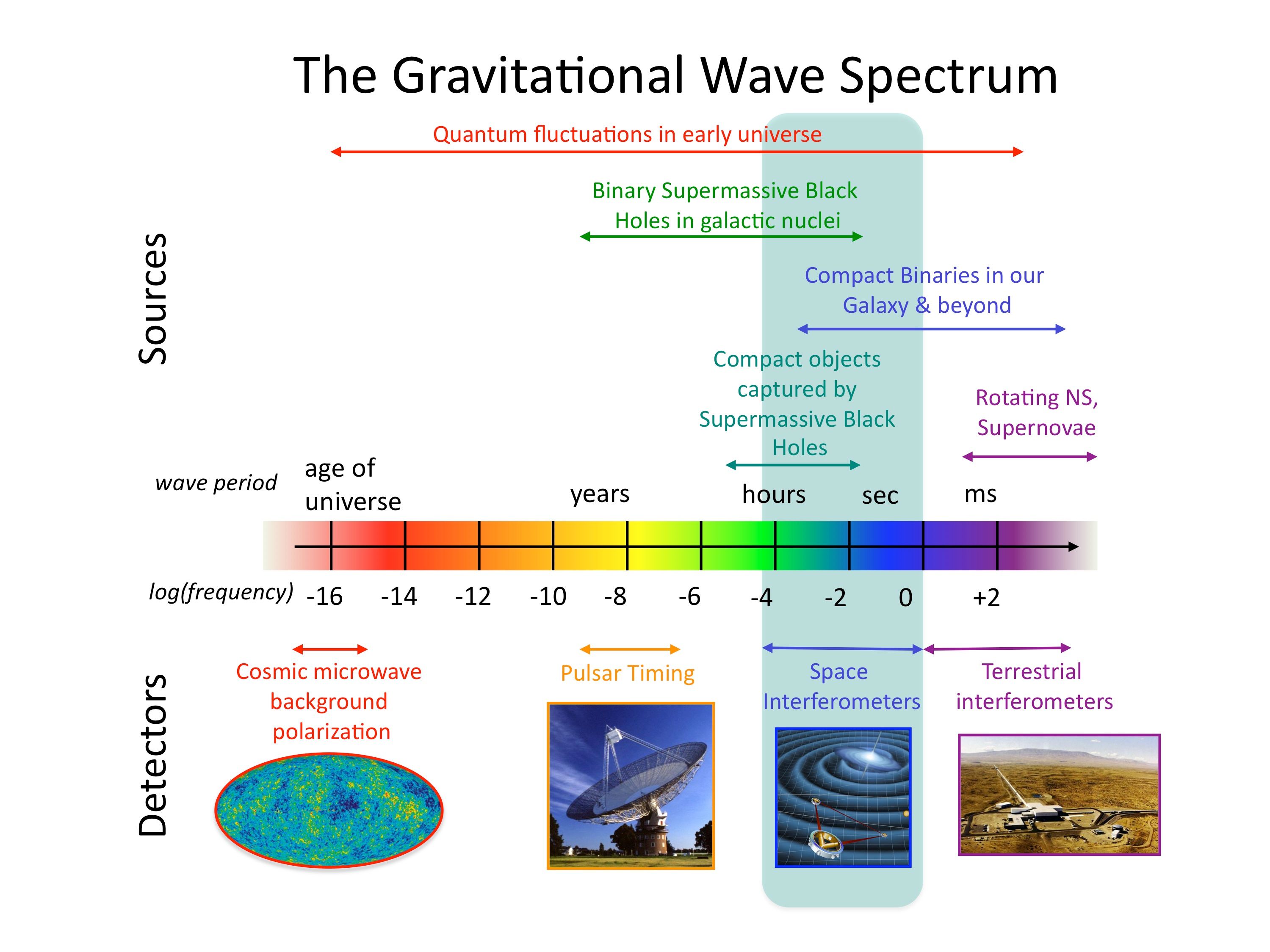