Second star to the right and straight on ’til morning—Astrophysics white papers

April 20, 2019August 1, 2020 / CPLB / Leave a comment

What will be the next big thing in astronomy? One of the hard things about research is that you often don’t know what you will discover before you embark on an investigation. An idea might work out, or it might not, or along the way you might discover something unexpected which is far more interesting. As you might imagine, this can make laying definite plans difficult…

However, it is important to have plans for research. While you might not be sure of the outcome, it is necessary to weigh the risks and rewards associated with the probable results before you invest your time and taxpayers’ money!

To help with planning and prioritising, researchers in astrophysics often pull together white papers [bonus note]. These are sketches of ideas for future research, arguing why you think they might be interesting. These can then be discussed within the community to help shape the direction of the field. If other scientists find the paper convincing, you can build support which helps push for funding. If there are gaps in the logic, others can point these out to ave you heading the wrong way. This type of consensus building is especially important for large experiments or missions—you don’t want to spend a billion dollars on something unless you’re really sure it is a good idea and lots of people agree.

I have been involved with a few white papers recently. Here are some key ideas for where research should go.

Ground-based gravitational-wave detectors: The next generation

We’ve done some awesome things with Advanced LIGO and Advanced Virgo. In just a couple of years we have revolutionized our understanding of binary black holes. That’s not bad. However, our current gravitational-wave observatories are limited in what they can detect. What amazing things could we achieve with a new generation of detectors?

It can take decades to develop new instruments, therefore it’s important to start thinking about them early. Obviously, what we would most like is an observatory which can detect everything, but that’s not feasible. In this white paper, we pick the questions we most want answered, and see what the requirements for a new detector would be. A design which satisfies these specifications would therefore be a solid choice for future investment.

Binary black holes are the perfect source for ground-based detectors. What do we most want to know about them?

How many mergers are there, and how does the merger rate change over the history of the Universe? We want to know how binary black holes are made. The merger rate encodes lots of information about how to make binaries, and comparing how this evolves compared with the rate at which the Universe forms stars, will give us a deeper understanding of how black holes are made.
What are the properties (masses and spins) of black holes? The merger rate tells us some things about how black holes form, but other properties like the masses, spins and orbital eccentricity complete the picture. We want to make precise measurements for individual systems, and also understand the population.
Where do supermassive black holes come from? We know that stars can collapse to produce stellar-mass black holes. We also know that the centres of galaxies contain massive black holes. Where do these massive black holes come from? Do they grow from our smaller black holes, or do they form in a different way? Looking for intermediate-mass black holes in the gap in-between will tells us whether there is a missing link in the evolution of black holes.

Detection horizon as a function of binary mass for Advanced LIGO, A+, Cosmic Explorer and the Einstein Telescope

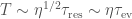
The detection horizon (the distance to which sources can be detected) for Advanced LIGO (aLIGO), its upgrade A+, and the proposed Cosmic Explorer (CE) and Einstein Telescope (ET). The horizon is plotted for binaries with equal-mass, nonspinning components. Adapted from Hall & Evans (2019).

What can we do to answer these questions?

Increase sensitivity! Advanced LIGO and Advanced Virgo can detect a $30 M_\odot + 30 M_\odot$ binary out to a redshift of about $z \approx 1$ . The planned detector upgrade A+ will see them out to redshift $z \approx 2$ . That’s pretty impressive, it means we’re covering 10 billion years of history. However, the peak in the Universe’s star formation happens at around $z \approx 2$ , so we’d really like to see beyond this in order to measure how the merger rate evolves. Ideally we would see all the way back to cosmic dawn at $z \approx 20$ when the Universe was only 200 million years old and the first stars light up.
Increase our frequency range! Our current detectors are limited in the range of frequencies they can detect. Pushing to lower frequencies helps us to detect heavier systems. If we want to detect intermediate-mass black holes of $100 M_\odot$ we need this low frequency sensitivity. At the moment, Advanced LIGO could get down to about $10~\mathrm{Hz}$ . The plot below shows the signal from a $100 M_\odot + 100 M_\odot$ binary at $z = 10$ . The signal is completely undetectable at $10~\mathrm{Hz}$ .
The gravitational wave signal from the final stages of inspiral, merger and ringdown of a two 100 solar mass black holes at a redshift of 10. The signal chirps up in frequency. The colour coding shows parts of the signal above different frequencies. Part of Figure 2 of the Binary Black Holes White Paper.
Increase sensitivity and frequency range! Increasing sensitivity means that we will have higher signal-to-noise ratio detections. For these loudest sources, we will be able to make more precise measurements of the source properties. We will also have more detections overall, as we can survey a larger volume of the Universe. Increasing the frequency range means we can observe a longer stretch of the signal (for the systems we currently see). This means it is easier to measure spin precession and orbital eccentricity. We also get to measure a wider range of masses. Putting the improved sensitivity and frequency range together means that we’ll get better measurements of individual systems and a more complete picture of the population.

How much do we need to improve our observatories to achieve our goals? To quantify this, lets consider the boost in sensitivity relative to A+, which I’ll call $\beta_\mathrm{A+}$ . If the questions can be answered with $\beta_\mathrm{A+} = 1$ , then we don’t need anything beyond the currently planned A+. If we need a slightly larger $\beta_\mathrm{A+}$ , we should start investigating extra ways to improve the A+ design. If we need much larger $\beta_\mathrm{A+}$ , we need to think about new facilities.

The plot below shows the boost necessary to detect a binary (with equal-mass nonspinning components) out to a given redshift. With a boost of $\beta_\mathrm{A+} = 10$ (blue line) we can survey black holes around $10 M_\odot$ – $30 M_\odot$ across cosmic time.

Boost to detect a binary of a given mass at a given redshift

The boost factor (relative to A+) $\beta_\mathrm{A+}$ needed to detect a binary with a total mass $M$ out to redshift $z$ . The binaries are assumed to have equal-mass, nonspinning components. The colour scale saturates at $\log_{10} \beta_\mathrm{A+} = 4.5$ . The blue curve highlights the reach at a boost factor of $\beta_\mathrm{A+} = 10$ . The solid and dashed white lines indicate the maximum reach of Cosmic Explorer and the Einstein Telescope, respectively. Part of Figure 1 of the Binary Black Holes White Paper.

The plot above shows that to see intermediate-mass black holes, we do need to completely overhaul the low-frequency sensitivity. What do we need to detect a $100 M_\odot + 100 M_\odot$ binary at $z = 10$ ? If we parameterize the noise spectrum (power spectral density) of our detector as $S_n(f) = S_{10}(f/10~\mathrm{Hz})^\alpha$ with a lower cut-off frequency of $f_\mathrm{min}$ , we can investigate the various possibilities. The plot below shows the possible combinations of parameters which meet of requirements.

Noise curve requirements for intermediate-mass black hole detection

Requirements on the low-frequency noise power spectrum necessary to detect an optimally oriented intermediate-mass binary black hole system with two 100 solar mass components at a redshift of 10. Part of Figure 2 of the Binary Black Holes White Paper.

To build up information about the population of black holes, we need lots of detections. Uncertainties scale inversely with the square root of the number of detections, so you would expect few percent uncertainty after 1000 detections. If we want to see how the population evolves, we need these many per redshift bin! The plot below shows the number of detections per year of observing time for different boost factors. The rate starts to saturate once we detect all the binaries in the redshift range. This is as good as you’ll ever going to get.

Detections per redshift bin as a function of boost factor

Expected rate of binary black hole detections $R_\mathrm{det}$ per redshift bin as a function of A+ boost factor $\beta_\mathrm{A+}$ for three redshift bins. The merging binaries are assumed to be uniformly distributed with a constant merger rate roughly consistent with current observations: the solid line is about the current median, while the dashed and dotted lines are roughly the 90% bounds. Figure 3 of the Binary Black Holes White Paper.

Looking at the plots above, it is clear that A+ is not going to satisfy our requirements. We need something with a boost factor of $\beta_\mathrm{A+} = 10$ : a next-generation observatory. Both the Cosmic Explorer and Einstein Telescope designs do satisfy our goals.

Data is pleased. Credit: Paramount

Title: Deeper, wider, sharper: Next-generation ground-based gravitational-wave observations of binary black holes
arXiv: 1903.09220 [astro-ph.HE]
Contribution level: ☆☆☆☆☆ Leading author
Theme music: Daft Punk

Extreme mass ratio inspirals are awesome

We have seen gravitational waves from a stellar-mass black hole merging with another stellar-mass black hole, can we observe a stellar-mass black hole merging with a massive black hole? Yes, these are a perfect source for a space-based gravitational wave observatory. We call these systems extreme mass-ratio inspirals (or EMRIs, pronounced em-rees, for short) [bonus note].

Having such an extreme mass ratio, with one black hole much bigger than the other, gives EMRIs interesting properties. The number of orbits over the course of an inspiral scales with the mass ratio: the more extreme the mass ratio, the more orbits there are. Each of these gives us something to measure in the gravitational wave signal.

The intricate structure of an EMRI orbit

A short section of an orbit around a spinning black hole. While inspirals last for years, this would represent only a few hours around a black hole of mass $M = 10^6 M_\odot$ . The position is measured in terms of the gravitational radius $r_\mathrm{g} = GM/c^2$ . The innermost stable orbit for this black hole would be about $r_\mathrm{g} = 2.3$ . Part of Figure 1 of the EMRI White Paper.

As EMRIs are so intricate, we can make exquisit measurements of the source properties. These will enable us to:

Measure the masses of both black holes to better than 10% precision
Reconstruct the mass distribution of massive black holes out to redshift $z \gtrsim 4$
Measure massive black hole spins to a precision of better than 0.001, giving us an insight into how they formed
Perform precision tests of the no-hair theorem describing black holes in general relativity, and test alternative theories of gravity in the strong-field regime
Cross-correlate locations with galaxy catalogues to measure the expansion of the Universe

Event rates for EMRIs are currently uncertain: there could be just one per year or thousands. From the rate we can figure out the details of what is going in in the nuclei of galaxies, and what types of objects you find there.

With EMRIs you can unravel mysteries in astrophysics, fundamental physics and cosmology.

Have we sold you that EMRIs are awesome? Well then, what do we need to do to observe them? There is only one currently planned mission which can enable us to study EMRIs: LISA. To maximise the science from EMRIs, we have to support LISA.

As an aspiring scientist, Lisa Simpson is a strong supporter of the LISA mission. Credit: Fox

Title: The unique potential of extreme mass-ratio inspirals for gravitational-wave astronomy
arXiv: 1903.03686 [astro-ph.HE]
Contribution level: ☆☆☆☆☆ Leading author
Theme music: Muse

Bonus notes

White paper vs journal article

Since white papers are proposals for future research, they aren’t as rigorous as usual academic papers. They are really attempts to figure out a good question to ask, rather than being answers. White papers are not usually peer reviewed before publication—the point is that you want everybody to comment on them, rather than just one or two anonymous referees.

Whilst white papers aren’t quite the same class as journal articles, they do still contain some interesting ideas, so I thought they still merit a blog post.

Recycling

I have blogged about EMRIs before, so I won’t go into too much detail here. It was one of my former blog posts which inspired the LISA Science Team to get in touch to ask me to write the white paper.

Science with the space-based interferometer LISA. V. Extreme mass-ratio inspirals

May 23, 2018June 15, 2018 / CPLB / Leave a comment

The space-based observatory LISA will detect gravitational waves from massive black holes (giant black holes residing in the centres of galaxies). One particularly interesting signal will come from the inspiral of a regular stellar-mass black hole into a massive black hole. These are called extreme mass-ratio inspirals (or EMRIs, pronounced emries, to their friends) [bonus note]. We have never observed such a system. This means that there’s a lot we have to learn about them. In this work, we systematically investigated the prospects for observing EMRIs. We found that even though there’s a wide range in predictions for what EMRIs we will detect, they should be a safe bet for the LISA mission.

Artistic impression of the spacetime for an extreme-mass-ratio inspiral, with a smaller stellar-mass black hole orbiting a massive black hole. This image is mandatory when talking about extreme-mass-ratio inspirals. Credit: NASA

LISA & EMRIs

My previous post discussed some of the interesting features of EMRIs. Because of the extreme difference in masses of the two black holes, it takes a long time for them to complete their inspiral. We can measure tens of thousands of orbits, which allows us to make wonderfully precise measurements of the source properties (if we can accurately pick out the signal from the data). Here, we’ll examine exactly what we could learn with LISA from EMRIs [bonus note].

First we build a model to investigate how many EMRIs there could be. There is a lot of astrophysics which we are currently uncertain about, which leads to a large spread in estimates for the number of EMRIs. Second, we look at how precisely we could measure properties from the EMRI signals. The astrophysical uncertainties are less important here—we could get a revolutionary insight into the lives of massive black holes.

The number of EMRIs

To build a model of how many EMRIs there are, we need a few different inputs:

The population of massive black holes
The distribution of stellar clusters around massive black holes
The range of orbits of EMRIs

We examine each of these in turn, building a more detailed model than has previously been constructed for EMRIs.

We currently know little about the population of massive black holes. This means we’ll discover lots when we start measuring signals (yay), but it’s rather inconvenient now, when we’re trying to predict how many EMRIs there are (boo). We take two different models for the mass distribution of massive black holes. One is based upon a semi-analytic model of massive black hole formation, the other is at the pessimistic end allowed by current observations. The semi-analytic model predicts massive black hole spins around 0.98, but we also consider spins being uniformly distributed between 0 and 1, and spins of 0. This gives us a picture of the bigger black hole, now we need the smaller.

Observations show that the masses of massive black holes are correlated with their surrounding cluster of stars—bigger black holes have bigger clusters. We consider four different versions of this trend: Gültekin et al. (2009); Kormendy & Ho (2013); Graham & Scott (2013), and Shankar et al. (2016). The stars and black holes about a massive black hole should form a cusp, with the density of objects increasing towards the massive black hole. This is great for EMRI formation. However, the cusp is disrupted if two galaxies (and their massive black holes) merge. This tends to happen—it’s how we get bigger galaxies (and black holes). It then takes some time for the cusp to reform, during which time, we don’t expect as many EMRIs. Therefore, we factor in the amount of time for which there is a cusp for massive black holes of different masses and spins.

That’s a nice galaxy you have there. It would be a shame if it were to collide with something… Hubble image of The Mice. Credit: ACS Science & Engineering Team.

Given a cusp about a massive black hole, we then need to know how often an EMRI forms. Simulations give us a starting point. However, these only consider a snap-shot, and we need to consider how things evolve with time. As stellar-mass black holes inspiral, the massive black hole will grow in mass and the surrounding cluster will become depleted. Both these effects are amplified because for each inspiral, there’ll be many more stars or stellar-mass black holes which will just plunge directly into the massive black hole. We therefore need to limit the number of EMRIs so that we don’t have an unrealistically high rate. We do this by adding in a couple of feedback factors, one to cap the rate so that we don’t deplete the cusp quicker than new objects will be added to it, and one to limit the maximum amount of mass the massive black hole can grow from inspirals and plunges. This gives us an idea for the total number of inspirals.

Finally, we calculate the orbits that EMRIs will be on. We again base this upon simulations, and factor in how the spin of the massive black hole effects the distribution of orbital inclinations.

Putting all the pieces together, we can calculate the population of EMRIs. We now need to work out how many LISA would be able to detect. This means we need models for the gravitational-wave signal. Since we are simulating a large number, we use a computationally inexpensive analytic model. We know that this isn’t too accurate, but we consider two different options for setting the end of the inspiral (where the smaller black hole finally plunges) which should bound the true range of results.

Number of EMRIs for different size massive black holes in different astrophysical models. M1 is our best estimate, the others explore variations on this. M11 and M12 are designed to be cover the extremes, being the most pessimistic and optimistic combinations. The solid and dashed lines are for two different signal models (AKK and AKS), which are designed to give an indication of potential variation. They agree where the massive black hole is not spinning (M10 and M11). The range of masses is similar for all models, as it is set by the sensitivity of LISA. We can detect higher mass systems assuming the AKK signal model as it includes extra inspiral close to highly spinning black holes: for the heaviest black holes, this is the only part of the signal at high enough frequency to be detectable. Figure 8 of Babak et al. (2017).

Allowing for all the different uncertainties, we find that there should be somewhere between 1 and 4200 EMRIs detected per year. (The model we used when studying transient resonances predicted about 250 per year, albeit with a slightly different detector configuration, which is fairly typical of all the models we consider here). This range is encouraging. The lower end means that EMRIs are a pretty safe bet, we’d be unlucky not to get at least one over the course of a multi-year mission (LISA should have at least four years observing). The upper end means there could be lots—we might actually need to worry about them forming a background source of noise if we can’t individually distinguish them!

EMRI measurements

Having shown that EMRIs are a good LISA source, we now need to consider what we could learn by measuring them?

We estimate the precision we will be able to measure parameters using the Fisher information matrix. The Fisher matrix measures how sensitive our observations are to changes in the parameters (the more sensitive we are, the better we should be able to measure that parameter). It should be a lower bound on actual measurement precision, and well approximate the uncertainty in the high signal-to-noise (loud signal) limit. The combination of our use of the Fisher matrix and our approximate signal models means our results will not be perfect estimates of real performance, but they should give an indication of the typical size of measurement uncertainties.

Given that we measure a huge number of cycles from the EMRI signal, we can make really precise measurements of the the mass and spin of the massive black hole, as these parameters control the orbital frequencies. Below are plots for the typical measurement precision from our Fisher matrix analysis. The orbital eccentricity is measured to similar accuracy, as it influences the range of orbital frequencies too. We also get pretty good measurements of the the mass of the smaller black hole, as this sets how quickly the inspiral proceeds (how quickly the orbital frequencies change). EMRIs will allow us to do precision astronomy!

Distribution of (one standard deviation) fractional uncertainties for measurements of the massive black hole (redshifted) mass $M_z$ . Results are shown for the different astrophysical models, and for the different signal models. The astrophysical model has little impact on the uncertainties. M4 shows a slight difference as it assumes heavier stellar-mass black holes. The results with the two signal models agree when the massive black hole is not spinning (M10 and M11). Otherwise, measurements are more precise with the AKK signal model, as this includes extra signal from the end of the inspiral. Part of Figure 11 of Babak et al. (2017).

Distribution of (one standard deviation) uncertainties for measurements of the massive black hole spin $a$ . The results mirror those for the masses above. Part of Figure 11 of Babak et al. (2017).

Now, before you get too excited that we’re going to learn everything about massive black holes, there is one confession I should make. In the plot above I show the measurement accuracy for the redshifted mass of the massive black hole. The cosmological expansion of the Universe causes gravitational waves to become stretched to lower frequencies in the same way light is (this makes visible light more red, hence the name). The measured frequency is $f_z = (1 + z)f$ where $f$ is the frequency emitted, and $z$ is the redshift ( $z= 0$ for a nearby source, and is larger for further away sources). Lower frequency gravitational waves correspond to higher mass systems, so it is often convenient to work with the redshifted mass, the mass corresponding to the signal you measure if you ignore redshifting. The redshifted mass of the massive black hole is $M_z = (1+z)M$ where $M$ is the true mass. To work out the true mass, we need the redshift, which means we need to measure the distance to the source.

Distribution of (one standard deviation) fractional uncertainties for measurements of the luminosity distance $D_\mathrm{L}$ . The signal model is not as important here, as the uncertainty only depends on how loud the signal is. Part of Figure 12 of Babak et al. (2017).

The plot above shows the fractional uncertainty on the distance. We don’t measure this too well, as it is determined from the amplitude of the signal, rather than its frequency components. The situation is much as for LIGO. The larger uncertainties on the distance will dominate the overall uncertainty on the black hole masses. We won’t be getting all these to fractions of a percent. However, that doesn’t mean we can’t still figure out what the distribution of masses looks like!

One of the really exciting things we can do with EMRIs is check that the signal matches our expectations for a black hole in general relativity. Since we get such an excellent map of the spacetime of the massive black hole, it is easy to check for deviations. In general relativity, everything about the black hole is fixed by its mass and spin (often referred to as the no-hair theorem). Using the measured EMRI signal, we can check if this is the case. One convenient way of doing this is to describe the spacetime of the massive object in terms of a multipole expansion. The first (most important) terms gives the mass, and the next term the spin. The third term (the quadrupole) is set by the first two, so if we can measure it, we can check if it is consistent with the expected relation. We estimated how precisely we could measure a deviation in the quadrupole. Fortunately, for this consistency test, all factors from redshifting cancel out, so we can get really detailed results, as shown below. Using EMRIs, we’ll be able to check for really small differences from general relativity!

EMRI measurement of bumpy black hole spacetime

Distribution of (one standard deviation) of uncertainties for deviations in the quadrupole moment of the massive object spacetime $\mathcal{Q}$ . Results are similar to the mass and spin measurements. Figure 13 of Babak et al. (2017).

In summary: EMRIS are awesome. We’re not sure how many we’ll detect with LISA, but we’re confident there will be some, perhaps a couple of hundred per year. From the signals we’ll get new insights into the masses and spins of black holes. This should tell us something about how they, and their surrounding galaxies, evolved. We’ll also be able to do some stringent tests of whether the massive objects are black holes as described by general relativity. It’s all pretty exciting, for when LISA launches, which is currently planned about 2034…

Sometimes, it leads to very little, and it seems like it's not worth it, and you wonder why you waited so long for something so disappointing

One of the most valuable traits a student or soldier can have: patience. Credit: Sony/Marvel

arXiv: 1703.09722 [gr-qc]
Journal: Physical Review D; 477(4):4685–4695; 2018
Conference proceedings: 1704.00009 [astro-ph.GA] (from when work was still in-progress)
Estimated number of Marvel films before LISA launch: 48 (starting with Ant-Man and the Wasp)

Bonus notes

Hyphenation

Is it “extreme-mass-ratio inspiral”, “extreme mass-ratio inspiral” or “extreme mass ratio inspiral”? All are used in the literature. This is one of the advantage of using “EMRI”. The important thing is that we’re talking about inspirals that have a mass ratio which is extreme. For this paper, we used “extreme mass-ratio inspiral”, but when I first started my PhD, I was first introduced to “extreme-mass-ratio inspirals”, so they are always stuck that way in my mind.

I think hyphenation is a bit of an art, and there’s no definitive answer here, just like there isn’t for superhero names, where you can have Iron Man, Spider-Man or Iceman.

Science with LISA

This paper is part of a series looking at what LISA could tells us about different gravitational wave sources. So far, this series covers

Massive black hole binaries
Cosmological phase transitions
Standard sirens (for measuring the expansion of the Universe)
Inflation
Extreme-mass-ratio inspirals

You’ll notice there’s a change in the name of the mission from eLISA to LISA part-way through, as things have evolved. (Or devolved?) I think the main take-away so far is that the cosmology group is the most enthusiastic.

Importance of transient resonances in extreme-mass-ratio inspirals

March 31, 2018July 5, 2018 / CPLB / Leave a comment

Extreme-mass-ratio inspirals (EMRIs for short) are a promising source for the planned space-borne gravitational-wave observatory LISA. To detect and analyse them we need accurate models for the signals, which are exquisitely intricate. In this paper, we investigated a feature, transient resonances, which have not previously included in our models. They are difficult to incorporate, but can have a big impact on the signal. Fortunately, we find that we can still detect the majority of EMRIs, even without including resonances. Phew!

EMRIs and orbits

EMRIs are a beautiful gravitational wave source. They occur when a stellar-mass black hole slowly inspirals into a massive black hole (as found in the centre of galaxies). The massive black hole can be tens of thousands or millions of times more massive than the stellar-mass black hole (hence extreme mass ratio). This means that the inspiral is slow—we can potentially measure tens of thousands of orbits. This is both the blessing and the curse of EMRIs. The huge numbers of cycles means that we can closely follow the inspiral, and build a detailed map of the massive black hole’s spacetime. EMRIs will give us precision measurements of the properties of massive black holes. However, to do this, we need to be able to find the EMRI signals in the data, we need models which can match the signals over all these cycles. Analysing EMRIs is a huge challenge.

EMRI orbits are complicated. At any moment, the orbit can be described by three orbital frequencies: one for radial (in/out) motion $\Omega_r$ , one for polar (north/south if we think of the spin of the massive black hole like the rotation of the Earth) motion $\Omega_\theta$ and one for axial (around in the east/west direction) motion. As gravitational waves are emitted, and the orbit shrinks, these frequencies evolve. 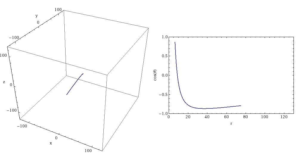The animation above, made by Steve Drasco, illustrates the evolution of an EMRI. Every so often, so can see the pattern freeze—the orbits stays in a constant shape (although this still rotates). This is a transient resonance. Two of the orbital frequencies become commensurate (so we might have 3 north/south cycles and 2 in/out cycles over the same period [bonus note])—this is the resonance. However, because the frequencies are still evolving, we don’t stay locked like this is forever—which is why the resonance is transient. To calculate an EMRI, you need to know how the orbital frequencies evolve.

The evolution of an EMRI is slow—the time taken to inspiral is much longer than the time taken to complete one orbit. Therefore, we can usually split the problem of calculating the trajectory of an EMRI into two parts. On short timescales, we can consider orbits as having fixed frequencies. On long timescale, we can calculate the evolution by averaging over many orbits. You might see the problem with this—around resonances, this averaging breaks down. Whereas normally averaging over many orbits means averaging over a complicated trajectory that hits pretty much all possible points in the orbital range, on resonance, you just average over the same bit again and again. On resonance, terms which usually average to zero can become important. Éanna Flanagan and Tanja Hinderer first pointed out that around resonances the usual scheme (referred to as the adiabatic approximation) doesn’t work.

A non-resonant EMRI orbit in three dimensions (left) and two dimensions (right), ignoring the rotation in the axial direction. A non-resonant orbit will eventually fill the $r$ – $\theta$ plane. Credit: Rob Cole

For comparison, a resonant EMRI orbit. A 2:3 resonance traces the same parts of the $r$ – $\theta$ plane over and over. Credit: Rob Cole

Around a resonance, the evolution will be enhanced or decreased a little relative to the standard adiabatic evolution. We get a kick. This is only small, but because we observe EMRIs for so many orbits, a small difference can grow to become a significant difference later on. Does this mean that we won’t be able to detect EMRIs with our standard models? This was a concern, so back at the end of PhD I began to investigate [bonus note]. The first step is to understand the size of the kick.

A jump in the orbital energy across a 2:3 resonance. The plot shows the difference between the approximate adiabatic evolution and the instantaneous evolution including the resonance. The thickness of the blue line is from oscillations on the orbital timescale which is too short to resolve here. The dotted red line shows the fitted size of the jump. Time is measured in terms of the resonance time $\tau_\mathrm{res}$ which is defined below. Figure 4 of Berry et al. (2016).

Resonance kicks

If there were no gravitational waves, the orbit would not evolve, it would be fixed. The orbit could then be described by a set of constants of motion. The most commonly used when describing orbits about black holes are the energy, angular momentum and Carter constant. For the purposes of this blog, we’ll not worry too much about what these constants are, we’ll just consider some constant $I$ .

The resonance kick is a change in this constant $\Delta I$ . What should this depend on? There are three ingredients. First, the rate of change of this constant $F$ on the resonant orbit. Second, the time spent on resonance $\tau_\mathrm{res}$ . The bigger these are, the bigger the size of the jump. Therefore,

$|\Delta I| \propto F \tau_\mathrm{res}$ .

However, the jump could be positive or negative. This depends upon the relative phase of the radial and polar motion [bonus note]—for example, do they both reach their maximum point at the same time, or does one lag behind the other? We’ll call this relative phase $q$ . By varying $q$ we explore we can get our resonant trajectory to go through any possible point in space. Therefore, averaging over $q$ should get us back to the adiabatic approximation: the average value of $\Delta I$ must be zero. To complete our picture for the jump, we need a periodic function of the phase,

$\Delta I = F \tau_\mathrm{res} f(q)$ ,

with $\langle f(q) \rangle_q = 0$ . Now, we know the pieces, we can try to figure out what the pieces are.

The rate of change $F$ is proportional the mass ratio $\eta \ll 1$ : the smaller the stellar-mass black hole is relative to the massive one, the smaller $F$ is. The exact details depend upon gravitational self-force calculations, which we’ll skip over, as they’re pretty hard, but they are the same for all orbits (resonant or not).

We can think of the resonance timescale either as the time for the orbital frequencies to drift apart or the time for the orbit to start filling the space again (so that it’s safe to average). The two pictures yield the same answer—there’s a fuller explanation in Section III A of the paper. To define the resonance timescale, it is useful to define the frequency $\Omega = n_r \Omega_r - n_\theta \Omega_\theta$ , which is zero exactly on resonance. If this is evolving at rate $\dot{\Omega}$ , then the resonance timescale is

$\displaystyle \tau_\mathrm{res} = \left[\frac{2\pi}{\dot{\Omega}}\right]^{1/2}$ .

This bridges the two timescales that usually define EMRIs: the short orbital timescale $T$ and the long evolution timescale $\tau_\mathrm{ev}$ :

$T \sim \eta^{1/2} \tau_\mathrm{res} \sim \eta \tau_\mathrm{ev}$ .

To find the form of for $f(q)$ , we need to do some quite involved maths (given in Appendix B of the paper) [bonus note]. This works by treating the evolution far from resonance as depending upon two independent times (effectively defining $T$ and $\tau_\mathrm{ev}$ ), and then matching the evolution close to resonance using an expansion in terms of a different time (something like $\tau_\mathrm{res}$ ). The solution shows that the jump depends sensitively upon the phase $q$ at resonance, which makes them extremely difficult to calculate.

We numerically evaluated the size of kicks for different orbits and resonances. We found a number of trends. First, higher-order resonances (those with larger $n_r$ and $n_\theta$ ) have smaller jumps than lower-order ones. This makes sense, as higher-order resonances come closer to covering all the points in the space, and so are more like averaging over the entire space. Second, jumps are larger for higher eccentricity orbits. This also makes sense, as you can’t have resonances for circular (zero eccentricity orbits) as there’s no radial frequency, so the size of the jumps must tend to zero. We’ll see that these two points are important when it comes to observational consequences of transient resonances.

Astrophysical EMRIs

Now we’ve figured out the impact of passing through a transient resonance, let’s look at what this means for detecting EMRIs. The jump can mean that the evolution post-resonance can soon become out of phase with that pre-resonance. We can’t match both parts with the same adiabatic template. This could significantly hamper our prospects for detection, as we’re limited to the bits of signal we can pick up between resonances.

We created an astrophysical population of simulated EMRIs. We used numerical simulations to estimate a plausible population of massive black holes and distribution of stellar-mass black holes insprialling into them. We then used adiabatic models to see how many LISA (or eLISA as it was called at the time) could potentially detect. We found there were ~510 EMRIs detectable (with a signal-to-noise ratio of 15 or above) for a two-year mission.

We then calculated how much the signal-to-noise ratio would be reduced by passing through transient resonances. The plot below shows the distribution of signal-to-noise ratio for the original population, ignoring resonances, and then after factoring in the reduction. There are now ~490 detectable EMRIs, a loss of 4%. We can still detect the majority of EMRIs!

Distribution of signal-to-noise ratios for EMRIs. In blue (solid outline), we have the results ignoring transient resonances. In orange (dashed outline), we have the distribution including the reduction due to resonance jumps. Events falling below 15 are deemed to be undetectable. Figure 10 of Berry et al. (2016).

We were worried about the impact of transient resonances, we know that jumps can cause them to become undetectable, so why aren’t we seeing a bit effect in our population? The answer lies is in the trends we saw earlier. Jumps are large for low order resonances with high eccentricities. These were the ones first highlighted, as they are obviously the most important. However, low-order resonances are only encountered really close to the massive black hole. This means late in the inspiral, after we have already accumulated lots of signal-to-noise ratio. Losing a little bit of signal right at the end doesn’t hurt detectability too much. On top of this, gravitational wave emission efficiently damps down eccentricity. Orbits typically have low eccentricities by the time they hit low-order resonances, meaning that the jumps are actually quite small. Although small jumps lead to some mismatch, we can still use our signal templates without jumps. Therefore, resonances don’t hamper us (too much) in finding EMRIs!

This may seem like a happy ending, but it is not the end of the story. While we can detect EMRIs, we still need to be able to accurately infer their source properties. Features not included in our signal templates (like jumps), could bias our results. For example, it might be that we can better match a jump by using a template for a different black hole mass or spin. However, if we include jumps, these extra features could give us extra precision in our measurements. The question of what jumps could mean for parameter estimation remains to be answered.

arXiv: 1608.08951 [gr-qc]
Journal: Physical Review D; 94(12):124042(24); 2016
Conference proceedings: 1702.05481 [gr-qc] (only 2 pages—ideal for emergency journal club presentations)
Favourite jumpers: Woolly, Mario, Kangaroos

Bonus notes

Radial and polar only

When discussing resonances, and their impact on orbital evolution, we’ll only care about $\Omega_r$ – $\Omega_\theta$ resonances. Resonances with $\Omega_\phi$ are not important because the spacetime is axisymmetric. The equations are exactly identical for all values of the the axial angle $\phi$ , so it doesn’t matter where you are (or if you keep cycling over the same spot) for the evolution of the EMRI.

This, however, doesn’t mean that $\Omega_\phi$ resonances aren’t interesting. They can lead to small kicks to the binary, because you are preferentially emitting gravitational waves in one direction. For EMRIs this are negligibly small, but for more equal mass systems, they could have some interesting consequences as pointed out by Maarten van de Meent.

Extra time

I’m grateful to the Cambridge Philosophical Society for giving me some extra funding to work on resonances. If you’re a Cambridge PhD student, make sure to become a member so you can take advantage of the opportunities they offer.

Calculating jumps

The theory of how to evolve through a transient resonance was developed by Kevorkian and coauthors. I spent a long time studying these calculations before working up the courage to attempt them myself. There are a few technical details which need to be adapted for the case of EMRIs. I finally figured everything out while in Warsaw Airport, coming back from a conference. It was the most I had ever felt like a real physicist.

Transient resonances remind me of Spirographs. Thanks Frinkiac

Inference on gravitational waves from coalescences of stellar-mass compact objects and intermediate-mass black holes

June 4, 2016August 27, 2016 / CPLB / Leave a comment

I love collecting things, there’s something extremely satisfying about completing a set. I suspect that this is one of the alluring features of Pokémon—you’ve gotta catch ’em all. The same is true of black hole hunting. Currently, we know of stellar-mass black holes which are a few times the mass of our Sun, up to a few tens of the mass of our Sun (the black holes of GW150914 are the biggest yet to be observed), and we know of supermassive black holes, which are ten thousand to ten billion times the mass our Sun. However, we are missing intermediate-mass black holes which lie in the middle. We have Charmander and Charizard, but where is Charmeleon? The elusive ones are always the most satisfying to capture.

Adorable black hole (available for adoption). I’m sure this could be a Pokémon. It would be a Dark type. Not that I’ve given it that much thought…

Intermediate-mass black holes have evaded us so far. We’re not even sure that they exist, although that would raise questions about how you end up with the supermassive ones (you can’t just feed the stellar-mass ones lots of rare candy). Astronomers have suggested that you could spot intermediate-mass black holes in globular clusters by the impact of their gravity on the motion of other stars. However, this effect would be small, and near impossible to conclusively spot. Another way (which I’ve discussed before), would to be to look at ultra luminous X-ray sources, which could be from a disc of material spiralling into the black hole. However, it’s difficult to be certain that we understand the source properly and that we’re not misclassifying it. There could be one sure-fire way of identifying intermediate-mass black holes: gravitational waves.

The frequency of gravitational waves depend upon the mass of the binary. More massive systems produce lower frequencies. LIGO is sensitive to the right range of frequencies for stellar-mass black holes. GW150914 chirped up to the pitch of a guitar’s open B string (just below middle C). Supermassive black holes produce gravitational waves at too low frequency for LIGO (a space-based detector would be perfect for these). We might just be able to detect signals from intermediate-mass black holes with LIGO.

In a recent paper, a group of us from Birmingham looked at what we could learn from gravitational waves from the coalescence of an intermediate-mass black hole and a stellar-mass black hole [bonus note]. We considered how well you would be able to measure the masses of the black holes. After all, to confirm that you’ve found an intermediate-mass black hole, you need to be sure of its mass.

The signals are extremely short: we only can detect the last bit of the two black holes merging together and settling down as a final black hole. Therefore, you might think there’s not much information in the signal, and we won’t be able to measure the properties of the source. We found that this isn’t the case!

We considered a set of simulated signals, and analysed these with our parameter-estimation code [bonus note]. Below are a couple of plots showing the accuracy to which we can infer a couple of different mass parameters for binaries of different masses. We show the accuracy of measuring the chirp mass $\mathcal{M}$ (a much beloved combination of the two component masses which we are usually able to pin down precisely) and the total mass $M_\mathrm{total}$ .

Measured chirp mass for systems of different total masses. The shaded regions show the 90% credible interval and the dashed lines show the true values. The mass ratio $q$ is the mass of the stellar-mass black hole divided by the mass of the intermediate-mass black hole. Figure 1 of Haster et al. (2016).

Measured total mass for systems of different total masses. The shaded regions show the 90% credible interval and the dashed lines show the true values. Figure 2 of Haster et al. (2016).

For the lower mass systems, we can measure the chirp mass quite well. This is because we get a little information from the part of the gravitational wave from when the two components are inspiralling together. However, we see less and less of this as the mass increases, and we become more and more uncertain of the chirp mass.

The total mass isn’t as accurately measured as the chirp mass at low masses, but we see that the accuracy doesn’t degrade at higher masses. This is because we get some constraints on its value from the post-inspiral part of the waveform.

We found that the transition from having better fractional accuracy on the chirp mass to having better fractional accuracy on the total mass happened when the total mass was around 200–250 solar masses. This was assuming final design sensitivity for Advanced LIGO. We currently don’t have as good sensitivity at low frequencies, so the transition will happen at lower masses: GW150914 is actually in this transition regime (the chirp mass is measured a little better).

Given our uncertainty on the masses, when can we conclude that there is an intermediate-mass black hole? If we classify black holes with masses more than 100 solar masses as intermediate mass, then we’ll be able to say to claim a discovery with 95% probability if the source has a black hole of at least 130 solar masses. The plot below shows our inferred probability of there being an intermediate-mass black hole as we increase the black hole’s mass (there’s little chance of falsely identifying a lower mass black hole).

Intermediate-mass black hole probability

Probability that the larger black hole is over 100 solar masses (our cut-off mass for intermediate-mass black holes $M_\mathrm{IMBH}$ ). Figure 7 of Haster et al. (2016).

Gravitational-wave observations could lead to a concrete detection of intermediate mass black holes if they exist and merge with another black hole. However, LIGO’s low frequency sensitivity is important for detecting these signals. If detector commissioning goes to plan and we are lucky enough to detect such a signal, we’ll finally be able to complete our set of black holes.

arXiv: 1511.01431 [astro-ph.HE]
Journal: Monthly Notices of the Royal Astronomical Society; 457(4):4499–4506; 2016
Birmingham science summary: Inference on gravitational waves from coalescences of stellar-mass compact objects and intermediate-mass black holes (by Carl)
Other collectables: Breakthrough, Gruber, Shaw, Kavli, …

Bonus notes

Jargon

The coalescence of an intermediate-mass black hole and a stellar-mass object (black hole or neutron star) has typically been known as an intermediate mass-ratio inspiral (an IMRI). This is similar to the name for the coalescence of a a supermassive black hole and a stellar-mass object: an extreme mass-ratio inspiral (an EMRI). However, my colleague Ilya has pointed out that with LIGO we don’t really see much of the intermediate-mass black hole and the stellar-mass black hole inspiralling together, instead we see the merger and ringdown of the final black hole. Therefore, he prefers the name intermediate mass-ratio coalescence (or IMRAC). It’s a better description of the signal we measure, but the acronym isn’t as good.

Parameter-estimation runs

The main parameter-estimation analysis for this paper was done by Zhilu, a summer student. This is notable for two reasons. First, it shows that useful research can come out of a summer project. Second, our parameter-estimation code installed and ran so smoothly that even an undergrad with no previous experience could get some useful results. This made us optimistic that everything would work perfectly in the upcoming observing run (O1). Unfortunately, a few improvements were made to the code before then, and we were back to the usual level of fun in time for The Event.

Christopher Berry

Gravitational-wave astronomer

EMRIs

Second star to the right and straight on ’til morning—Astrophysics white papers