Gravitational-wave astronomy lets us observing binary black holes. These systems, being made up of two black holes, are pretty difficult to study by any other means. It has long been argued that with this new information we can unravel the mysteries of stellar evolution. Just as a palaeontologist can discover how long-dead animals lived from their bones, we can discover how massive stars lived by studying their black hole remnants. In this paper, we quantify how much we can really learn from this black hole palaeontology—after 1000 detections, we should pin down some of the most uncertain parameters in binary evolution to a few percent precision.
Life as a binary
There are many proposed ways of making a binary black hole. The current leading contender is isolated binary evolution: start with a binary star system (most stars are in binaries or higher multiples, our lonesome Sun is a little unusual), and let the stars evolve together. Only a fraction will end with black holes close enough to merge within the age of the Universe, but these would be the sources of the signals we see with LIGO and Virgo. We consider this isolated binary scenario in this work [bonus note].
Now, you might think that with stars being so fundamentally important to astronomy, and with binary stars being so common, we’d have the evolution of binaries figured out by now. It turns out it’s actually pretty messy, so there’s lots of work to do. We consider constraining four parameters which describe the bits of binary physics which we are currently most uncertain of:
Black hole natal kicks—the push black holes receive when they are born in supernova explosions. We now the neutron stars get kicks, but we’re less certain for black holes [bonus note].
Common envelope efficiency—one of the most intricate bits of physics about binaries is how mass is transferred between stars. As they start exhausting their nuclear fuel they puff up, so material from the outer envelope of one star may be stripped onto the other. In the most extreme cases, a common envelope may form, where so much mass is piled onto the companion, that both stars live in a single fluffy envelope. Orbiting inside the envelope helps drag the two stars closer together, bringing them closer to merging. The efficiency determines how quickly the envelope becomes unbound, ending this phase.
Mass loss rates during the Wolf–Rayet (not to be confused with Wolf 359) and luminous blue variable phases–stars lose mass through out their lives, but we’re not sure how much. For stars like our Sun, mass loss is low, there is enough to gives us the aurora, but it doesn’t affect the Sun much. For bigger and hotter stars, mass loss can be significant. We consider two evolutionary phases of massive stars where mass loss is high, and currently poorly known. Mass could be lost in clumps, rather than a smooth stream, making it difficult to measure or simulate.
We use parameters describing potential variations in these properties are ingredients to the COMPAS population synthesis code. This rapidly (albeit approximately) evolves a population of stellar binaries to calculate which will produce merging binary black holes.
The question is now which parameters affect our gravitational-wave measurements, and how accurately we can measure those which do?
Binary black hole merger rate at three different redshifts as calculated by COMPAS. We show the rate in 30 different chirp mass bins for our default population parameters. The caption gives the total rate for all masses. Figure 2 of Barrett et al. (2018)
Gravitational-wave observations
For our deductions, we use two pieces of information we will get from LIGO and Virgo observations: the total number of detections, and the distributions of chirp masses. The chirp mass is a combination of the two black hole masses that is often well measured—it is the most important quantity for controlling the inspiral, so it is well measured for low mass binaries which have a long inspiral, but is less well measured for higher mass systems. In reality we’ll have much more information, so these results should be the minimum we can actually do.
We consider the population after 1000 detections. That sounds like a lot, but we should have collected this many detections after just 2 or 3 years observing at design sensitivity. Our default COMPAS model predicts 484 detections per year of observing time! Honestly, I’m a little scared about having this many signals…
For a set of population parameters (black hole natal kick, common envelope efficiency, luminous blue variable mass loss and Wolf–Rayet mass loss), COMPAS predicts the number of detections and the fraction of detections as a function of chirp mass. Using these, we can work out the probability of getting the observed number of detections and fraction of detections within different chirp mass ranges. This is the likelihood function: if a given model is correct we are more likely to get results similar to its predictions than further away, although we expect their to be some scatter.
If you like equations, the from of our likelihood is explained in this bonus note. If you don’t like equations, there’s one lurking in the paragraph below. Just remember, that it can’t see you if you don’t move. It’s OK to skip the equation.
To determine how sensitive we are to each of the population parameters, we see how the likelihood changes as we vary these. The more the likelihood changes, the easier it should be to measure that parameter. We wrap this up in terms of the Fisher information matrix. This is defined as
,
where is the likelihood for data (the number of observations and their chirp mass distribution in our case), are our parameters (natal kick, etc.), and the angular brackets indicate the average over the population parameters. In statistics terminology, this is the variance of the score, which I think sounds cool. The Fisher information matrix nicely quantifies how much information we can lean about the parameters, including the correlations between them (so we can explore degeneracies). The inverse of the Fisher information matrix gives a lower bound on the covariance matrix (the multidemensional generalisation of the variance in a normal distribution) for the parameters . In the limit of a large number of detections, we can use the Fisher information matrix to estimate the accuracy to which we measure the parameters [bonus note].
We simulated several populations of binary black hole signals, and then calculate measurement uncertainties for our four population uncertainties to see what we could learn from these measurements.
Results
Using just the rate information, we find that we can constrain a combination of the common envelope efficiency and the Wolf–Rayet mass loss rate. Increasing the common envelope efficiency ends the common envelope phase earlier, leaving the binary further apart. Wider binaries take longer to merge, so this reduces the merger rate. Similarly, increasing the Wolf–Rayet mass loss rate leads to wider binaries and smaller black holes, which take longer to merge through gravitational-wave emission. Since the two parameters have similar effects, they are anticorrelated. We can increase one and still get the same number of detections if we decrease the other. There’s a hint of a similar correlation between the common envelope efficiency and the luminous blue variable mass loss rate too, but it’s not quite significant enough for us to be certain it’s there.
Fisher information matrix estimates for fractional measurement precision of the four population parameters: the black hole natal kick , the common envelope efficiency , the Wolf–Rayet mass loss rate , and the luminous blue variable mass loss rate . There is an anticorrealtion between and , and hints at a similar anticorrelation between and . We show 1500 different realisations of the binary population to give an idea of scatter. Figure 6 of Barrett et al. (2018)
Adding in the chirp mass distribution gives us more information, and improves our measurement accuracies. The fraction uncertainties are about 2% for the two mass loss rates and the common envelope efficiency, and about 5% for the black hole natal kick. We’re less sensitive to the natal kick because the most massive black holes don’t receive a kick, and so are unaffected by the kick distribution [bonus note]. In any case, these measurements are exciting! With this type of precision, we’ll really be able to learn something about the details of binary evolution.
Measurement precision for the four population parameters after 1000 detections. We quantify the precision with the standard deviation estimated from the Fisher inforamtion matrix. We show results from 1500 realisations of the population to give an idea of scatter. Figure 5 of Barrett et al. (2018)
The accuracy of our measurements will improve (on average) with the square root of the number of gravitational-wave detections. So we can expect 1% measurements after about 4000 observations. However, we might be able to get even more improvement by combining constraints from other types of observation. Combining different types of observation can help break degeneracies. I’m looking forward to building a concordance model of binary evolution, and figuring out exactly how massive stars live their lives.
In practise, we will need to worry about how binary black holes are formed, via isolated evolution or otherwise, before inferring the parameters describing binary evolution. This makes the problem more complicated. Some parameters, like mass loss rates or black hole natal kicks, might be common across multiple channels, while others are not. There are a number of ways we might be able to tell different formation mechanisms apart, such as by using spin measurements.
Kick distribution
We model the supernova kicks as following a Maxwell–Boltzmann distribution,
,
where is the unknown population parameter. The natal kick received by the black hole is not the same as this, however, as we assume some of the material ejected by the supernova falls back, reducing the over kick. The final natal kick is
,
where is the fraction that falls back, taken from Fryer et al. (2012). The fraction is greater for larger black holes, so the biggest black holes get no kicks. This means that the largest black holes are unaffected by the value of .
The likelihood
In this analysis, we have two pieces of information: the number of detections, and the chirp masses of the detections. The first is easy to summarise with a single number. The second is more complicated, and we consider the fraction of events within different chirp mass bins.
Our COMPAS model predicts the merger rate and the probability of falling in each chirp mass bin (we factor measurement uncertainty into this). Our observations are the the total number of detections and the number in each chirp mass bin (). The likelihood is the probability of these observations given the model predictions. We can split the likelihood into two pieces, one for the rate, and one for the chirp mass distribution,
.
For the rate likelihood, we need the probability of observing given the predicted rate . This is given by a Poisson distribution,
,
where is the total observing time. For the chirp mass likelihood, we the probability of getting a number of detections in each bin, given the predicted fractions. This is given by a multinomial distribution,
.
These look a little messy, but they simplify when you take the logarithm, as we need to do for the Fisher information matrix.
When we substitute in our likelihood into the expression for the Fisher information matrix, we get
.
Conveniently, although we only need to evaluate first-order derivatives, even though the Fisher information matrix is defined in terms of second derivatives. The expected number of events is . Therefore, we can see that the measurement uncertainty defined by the inverse of the Fisher information matrix, scales on average as .
For anyone worrying about using the likelihood rather than the posterior for these estimates, the high number of detections [bonus note] should mean that the information we’ve gained from the data overwhelms our prior, meaning that the shape of the posterior is dictated by the shape of the likelihood.
Interpretation of the Fisher information matrix
As an alternative way of looking at the Fisher information matrix, we can consider the shape of the likelihood close to its peak. Around the maximum likelihood point, the first-order derivatives of the likelihood with respect to the population parameters is zero (otherwise it wouldn’t be the maximum). The maximum likelihood values of and are the same as their expectation values. The second-order derivatives are given by the expression we have worked out for the Fisher information matrix. Therefore, in the region around the maximum likelihood point, the Fisher information matrix encodes all the relevant information about the shape of the likelihood.
So long as we are working close to the maximum likelihood point, we can approximate the distribution as a multidimensional normal distribution with its covariance matrix determined by the inverse of the Fisher information matrix. Our results for the measurement uncertainties are made subject to this approximation (which we did check was OK).
Approximating the likelihood this way should be safe in the limit of large . As we get more detections, statistical uncertainties should reduce, with the peak of the distribution homing in on the maximum likelihood value, and its width narrowing. If you take the limit of , you’ll see that the distribution basically becomes a delta function at the maximum likelihood values. To check that our was large enough, we verified that higher-order derivatives were still small.
Michele Vallisneri has a good paper looking at using the Fisher information matrix for gravitational wave parameter estimation (rather than our problem of binary population synthesis). There is a good discussion of its range of validity. The high signal-to-noise ratio limit for gravitational wave signals corresponds to our high number of detections limit.
Gravitational waves allow us to infer the properties of binary black holes (two black holes in orbit about each other), but can we use this information to figure out how the black holes and the binary form? In this paper, we show that measurements of the black holes’ spins can help us this out, but probably not until we have at least 100 detections.
Black hole spins
Black holes are described by their masses (how much they bend spacetime) and their spins (how much they drag spacetime to rotate about them). The orientation of the spins relative to the orbit of the binary could tell us something about the history of the binary [bonus note].
We considered four different populations of spin–orbit alignments to see if we could tell them apart with gravitational-wave observations:
Aligned—matching the idealised example of isolated binary evolution. This stands in for the case where misalignments are small, which might be the case if material blown off during a supernova ends up falling back and being swallowed by the black hole.
Isotropic—matching the expectations for dynamically formed binaries.
Equal misalignments at birth—this would be the case if the spins and orbit were aligned before the second supernova, which then tilted the plane of the orbit. (As the binary inspirals, the spins wobble around, so the two misalignment angles won’t always be the same).
Both spins misaligned by supernova kicks, assuming that the stars were aligned with the orbit before exploding. This gives a more general scatter of unequal misalignments, but typically the primary (bigger and first forming) black hole is more misaligned.
These give a selection of possible spin alignments. For each, we assumed that the spin magnitude was the same and had a value of 0.7. This seemed like a sensible idea when we started this study [bonus note], but is now towards the upper end of what we expect for binary black holes.
Hierarchical analysis
To measurement the properties of the population we need to perform a hierarchical analysis: there are two layers of inference, one for the individual binaries, and one of the population.
From a gravitational wave signal, we infer the properties of the source using Bayes’ theorem. Given the data , we want to know the probability that the parameters have different values, which is written as . This is calculated using
,
where is the likelihood, which we can calculate from our knowledge of the noise in our gravitational wave detectors, is the prior on the parameters (what we would have guessed before we had the data), and the normalisation constant is called the evidence. We’ll use the evidence again in the next layer of inference.
Our prior on the parameters should actually depend upon what we believe about the astrophysical population. It is different if we believed that Model 1 were true (when we’d only consider aligned spins) than for Model 2. Therefore, we should really write
,
where denotes which model we are considering.
This is an important point to remember: if you our using our LIGO results to test your theory of binary formation, you need to remember to correct for our choice of prior. We try to pick non-informative priors—priors that don’t make strong assumptions about the physics of the source—but this doesn’t mean that they match what would be expected from your model.
We are interested in the probability distribution for the different models: how many binaries come from each. Given a set of different observations , we can work this out using another application of Bayes’ theorem (yay)
,
where is just all the evidences for the individual events (given that model) multiplied together, is our prior for the different models, and is another normalisation constant.
Now knowing how to go from a set of observations to the probability distribution on the different channels, let’s give it a go!
Results
To test our approach made a set of mock gravitational wave measurements. We generated signals from binaries for each of our four models, and analysed these as we would for real signals (using LALInference). This is rather computationally expensive, and we wanted a large set of events to analyse, so using these results as a guide, we created a larger catalogue of approximate distributions for the inferred source parameters . We then fed these through our hierarchical analysis. The GIF below shows how measurements of the fraction of binaries from each population tightens up as we get more detections: the true fraction is marked in blue.
Probability distribution for the fraction of binaries from each of our four spin misalignment populations for different numbers of observations. The blue dot marks the true fraction: and equal fraction from all four channels.
The plot shows that we do zoom in towards the true fraction of events from each model as the number of events increases, but there are significant degeneracies between the different models. Notably, it is difficult to tell apart Models 1 and 3, as both have strong support for both spins being nearly aligned. Similarly, there is a degeneracy between Models 2 and 4 as both allow for the two spins to have very different misalignments (and for the primary spin, which is the better measured one, to be quite significantly misaligned).
This means that we should be able to distinguish aligned from misaligned populations (we estimated that as few as 5 events would be needed to distinguish the case that all events came from either Model 1 or Model 2 if those were the only two allowed possibilities). However, it will be more difficult to distinguish different scenarios which only lead to small misalignments from each other, or disentangle whether there is significant misalignment due to big supernova kicks or because binaries are formed dynamically.
The uncertainty of the fraction of events from each model scales roughly with the square root of the number of observations, so it may be slow progress making these measurements. I’m not sure whether we’ll know the answer to how binary black hole form, or who will sit on the Iron Throne first.
If you have two stars forming in a binary together, you’d expect them to be spinning in roughly the same direction, rotating the same way as they go round in their orbit (like our Solar System). This is because they all formed from the same cloud of swirling gas and dust. Furthermore, if two stars are to form a black hole binary that we can detect gravitational waves from, they need to be close together. This means that there can be tidal forces which gently tug the stars to align their rotation with the orbit. As they get older, stars puff up, meaning that if you have a close-by neighbour, you can share outer layers. This transfer of material will tend to align rotate too. Adding this all together, if you have an isolated binary of stars, you might expect that when they collapse down to become black holes, their spins are aligned with each other and the orbit.
Unfortunately, real astrophysics is rarely so clean. Even if the stars were initially rotating the same way as each other, they doesn’t mean that their black hole remnants will do the same. This depends upon how the star collapses. Massive stars explode as supernova, blasting off their outer layers while their cores collapse down to form black holes. Escaping material could carry away angular momentum, meaning that the black hole is spinning in a different direction to its parent star, or material could be blasted off asymmetrically, giving the new black hole a kick. This would change the plane of the binary’s orbit, misaligning the spins.
Alternatively, the binary could be formed dynamically. Instead of two stars living their lives together, we could have two stars (or black holes) come close enough together to form a binary. This is likely to happen in regions where there’s a high density of stars, such as a globular cluster. In this case, since the binary has been randomly assembled, there’s no reason for the spins to be aligned with each other or the orbit. For dynamically assembled binaries, all spin–orbit misalignments are equally probable.
Slow and steady
This project was led by Simon Stevenson. It was one of the first things we started working on at the beginning of his PhD. He has now graduated, and is off to start a new exciting life as a postdoc in Australia. We got a little distracted by other projects, most notably analysing the first detections of gravitational waves. Simon spent a lot of time developing the COMPAS population code, a code to simulate the evolution of binaries. Looking back, it’s impressive how far he’s come. This paper used a simple approximation to to estimate the masses of our black holes: we called it the Post-it note model, as we wrote it down on a single Post-it. Now Simon’s writing papers including the complexities of common-envelope evolution in order to explain LIGO’s actual observations.
On 4 January 2017, Advanced LIGO made a new detection of gravitational waves. The signal, which we call GW170104 [bonus note], came from the coalescence of two black holes, which inspiralled together (making that characteristic chirp) and then merged to form a single black hole.
On 4 January 2017, I was just getting up off the sofa when my phone buzzed. My new year’s resolution was to go for a walk every day, and I wanted to make use of the little available sunlight. However, my phone informed me that PyCBC (one or our search algorithms for signals from coalescing binaries) had identified an interesting event. I sat back down. I was on the rota to analyse interesting signals to infer their properties, and I was pretty sure that people would be eager to see results. They were. I didn’t leave the sofa for the rest of the day, bringing my new year’s resolution to a premature end.
Since 4 January, my time has been dominated by working on GW170104 (you might have noticed a lack of blog posts). Below I’ll share some of my war stories from life on the front line of gravitational-wave astronomy, and then go through some of the science we’ve learnt. (Feel free to skip straight to the science, recounting the story was more therapy for me).
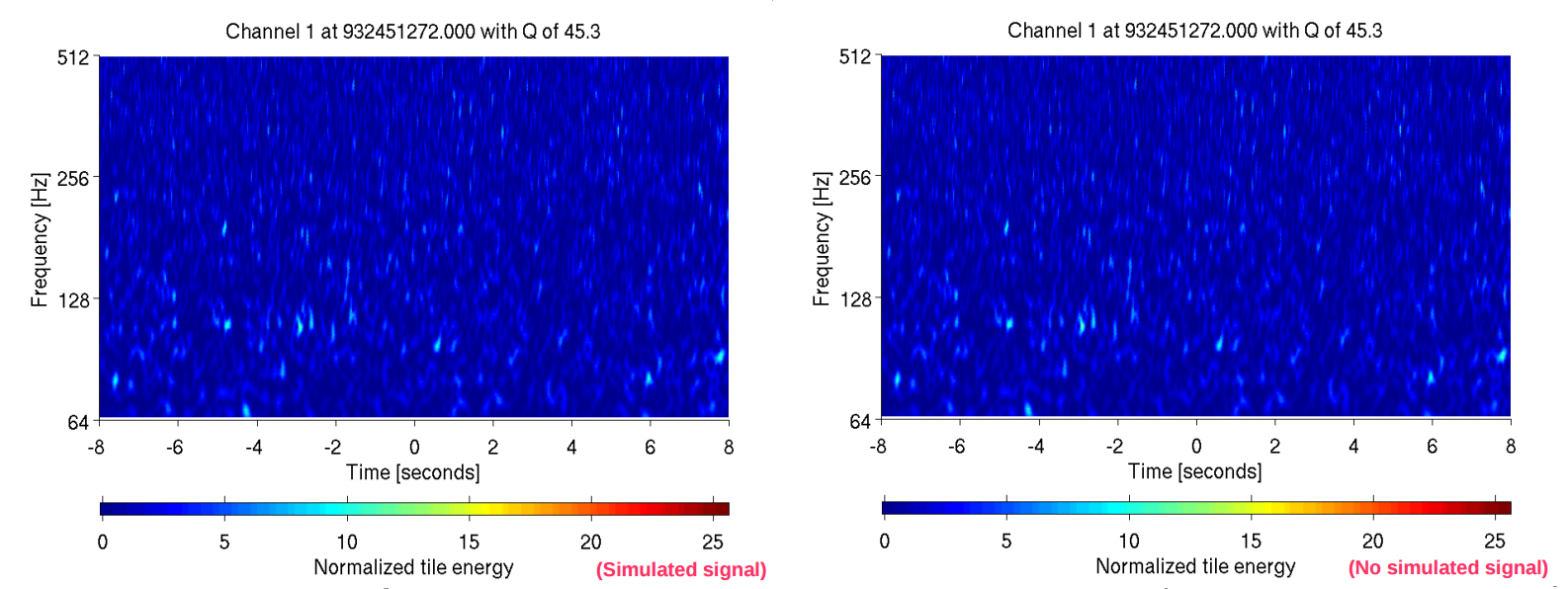
Time–frequency plots for GW170104 as measured by Hanford (top) and Livingston (bottom). The signal is clearly visible as the upward sweeping chirp. The loudest frequency is something between E3 and G♯3 on a piano, and it tails off somewhere between D♯4/E♭4 and F♯4/G♭4. Part of Fig. 1 of the GW170104 Discovery Paper.
The story
In the second observing run, the Parameter Estimation group have divided up responsibility for analysing signals into two week shifts. For each rota shift, there is an expert and a rookie. I had assumed that the first slot of 2017 would be a quiet time. The detectors were offline over the holidays, due back online on 4 January, but the instrumentalists would probably find some extra tinkering they’d want to do, so it’d probably slip a day, and then the weather would be bad, so we’d probably not collect much data anyway… I was wrong. Very wrong. The detectors came back online on time, and there was a beautifully clean detection on day one.
My partner for the rota was Aaron Zimmerman. 4 January was his first day running parameter estimation on live signals. I think I would’ve run and hidden underneath my duvet in his case (I almost did anyway, and I lived through the madness of our first detection GW150914), but he rose to the occasion. We had first results after just a few hours, and managed to send out a preliminary sky localization to our astronomer partners on 6 January. I think this was especially impressive as there were some difficulties with the initial calibration of the data. This isn’t a problem for the detection pipelines, but does impact the parameters which we infer, particularly the sky location. The Calibration group worked quickly, and produced two updates to the calibration. We therefore had three different sets of results (one per calibration) by 6 January [bonus note]!
Producing the final results for the paper was slightly more relaxed. Aaron and I conscripted volunteers to help run all the various permutations of the analysis we wanted to double-check our results [bonus note].
Recovered gravitational waveforms from analysis of GW170104. The broader orange band shows our estimate for the waveform without assuming a particular source (wavelet). The narrow blue bands show results if we assume it is a binary black hole (BBH) as predicted by general relativity. The two match nicely, showing no evidence for any extra features not included in the binary black hole models. Figure 4 of the GW170104 Discovery Paper.
I started working on GW170104 through my parameter estimation duties, and continued with paper writing.
Ahead of the second observing run, we decided to assemble a team to rapidly write up any interesting binary detections, and I was recruited for this (I think partially because I’m not too bad at writing and partially because I was in the office next to John Veitch, one of the chairs of the Compact Binary Coalescence group,so he can come and check that I wasn’t just goofing off eating doughnuts). We soon decided that we should write a paper about GW170104, and you can decide whether or not we succeeded in doing this rapidly…
Being on the paper writing team has given me huge respect for the teams who led the GW150914 and GW151226 papers. It is undoubtedly one of the most difficult things I’ve ever done. It is extremely hard to absorb negative remarks about your work continuously for months [bonus note]—of course people don’t normally send comments about things that they like, but that doesn’t cheer you up when you’re staring at an inbox full of problems that need fixing. Getting a collaboration of 1000 people to agree on a paper is like herding cats while being a small duckling.
On of the first challenges for the paper writing team was deciding what was interesting about GW170104. It was another binary black hole coalescence—aren’t people getting bored of them by now? The signal was quieter than GW150914, so it wasn’t as remarkable. However, its properties were broadly similar. It was suggested that perhaps we should title the paper “GW170104: The most boring gravitational-wave detection”.
One potentially interesting aspect was that GW170104 probably comes from greater distance than GW150914 or GW151226 (but perhaps not LVT151012) [bonus note]. This might make it a good candidate for testing for dispersion of gravitational waves.
Dispersion occurs when different frequencies of gravitational waves travel at different speeds. A similar thing happens for light when travelling through some materials, which leads to prisms splitting light into a spectrum (and hence the creation of Pink Floyd album covers). Gravitational waves don’t suffered dispersion in general relativity, but do in some modified theories of gravity.
It should be easier to spot dispersion in signals which have travelled a greater distance, as the different frequencies have had more time to separate out. Hence, GW170104 looks pretty exciting. However, being further away also makes the signal quieter, and so there is more uncertainty in measurements and it is more difficult to tell if there is any dispersion. Dispersion is also easier to spot if you have a larger spread of frequencies, as then there can be more spreading between the highest and lowest frequencies. When you throw distance, loudness and frequency range into the mix, GW170104 doesn’t always come out on top, depending upon the particular model for dispersion: sometimes GW150914’s loudness wins, other times GW151226’s broader frequency range wins. GW170104 isn’t too special here either.
Even though GW170104 didn’t look too exciting, we started work on a paper, thinking that we would just have a short letter describing our observations. The Compact Binary Coalescence group decided that we only wanted a single paper, and we wouldn’t bother with companion papers as we did for GW150914. As we started work, and dug further into our results, we realised that actually there was rather a lot that we could say.
I guess the moral of the story is that even though you might be overshadowed by the achievements of your siblings, it doesn’t mean that you’re not awesome. There might not be one outstanding feature of GW170104, but there are lots of little things that make it interesting. We are still at the beginning of understanding the properties of binary black holes, and each new detection adds a little more to our picture.
I think GW170104 is rather neat, and I hope you do too.
As we delved into the details of our results, we realised there was actually a lot of things that we could say about GW170104, especially when considered with our previous observations. We ended up having to move some of the technical details and results to Supplemental Material. With hindsight, perhaps it would have been better to have a companion paper or two. However, I rather like how packed with science this paper is.
The paper, which Physical Review Letters have kindly accommodated, despite its length, might not be as polished a classic as the GW150914 Discovery Paper, but I think they are trying to do different things. I rarely ever refer to the GW150914 Discovery Paper for results (more commonly I use it for references), whereas I think I’ll open up the GW170104 Discovery Paper frequently to look up numbers.
Although perhaps not right away, I’d quite like some time off first. The weather’s much better now, perfect for walking…
Advanced LIGO’s first observing run was hugely successful. Running from 12 September 2015 until 19 January 2016, there were two clear gravitational-wave detections, GW1501914 and GW151226, as well as a less certain candidate signal LVT151012. All three (assuming that they are astrophysical signals) correspond to the coalescence of binary black holes.
The second observing run started 30 November 2016. Following the first observing run’s detections, we expected more binary black hole detections. On 4 January, after we had collected almost 6 days’ worth of coincident data from the two LIGO instruments [bonus note], there was a detection.
The searches
The signal was first spotted by an online analysis. Our offline analysis of the data (using refined calibration and extra information about data quality) showed that the signal, GW170104, is highly significant. For both GstLAL and PyCBC, search algorithms which use templates to search for binary signals, the false alarm rate is estimated to be about 1 per 70,000 years.
The signal is also found in unmodelled (burst) searches, which look for generic, short gravitational wave signals. Since these are looking for more general signals than just binary coalescences, the significance associated with GW170104 isn’t as great, and coherent WaveBurst estimates a false alarm rate of 1 per 20,000 years. This is still pretty good! Reconstructions of the waveform from unmodelled analyses also match the form expected for binary black hole signals.
The search false alarm rates are the rate at which you’d expect something this signal-like (or more signal-like) due to random chance, if you data only contained noise and no signals. Using our knowledge of the search pipelines, and folding in some assumptions about the properties of binary black holes, we can calculate a probability that GW170104 is a real astrophysical signal. This comes out to be greater than .
The source
As for the previous gravitational wave detections, GW170104 comes from a binary black hole coalescence. The initial black holes were and (where is the mass of our Sun), and the final black hole was . The quoted values are the median values and the error bars denote the central 90% probable range. The plot below shows the probability distribution for the masses; GW170104 neatly nestles in amongst the other events.
Estimated masses for the two black holes in the binary . The two-dimensional shows the probability distribution for GW170104 as well as 50% and 90% contours for all events. The one-dimensional plot shows results using different waveform models. The dotted lines mark the edge of our 90% probability intervals. Figure 2 of the GW170104 Discovery Paper.
GW150914 was the first time that we had observed stellar-mass black holes with masses greater than around . GW170104 has similar masses, showing that our first detection was not a fluke, but there really is a population of black holes with masses stretching up into this range.
Black holes have two important properties: mass and spin. We have good measurements on the masses of the two initial black holes, but not the spins. The sensitivity of the form of the gravitational wave to spins can be described by two effective spin parameters, which are mass-weighted combinations of the individual spins.
The effective inspiral spin parameter qualifies the impact of the spins on the rate of inspiral, and where the binary plunges together to merge. It ranges from +1, meaning both black holes are spinning as fast as possible and rotate in the same direction as the orbital motion, to −1, both black holes spinning as fast as possible but in the opposite direction to the way that the binary is orbiting. A value of 0 for could mean that the black holes are not spinning, that their rotation axes are in the orbital plane (instead of aligned with the orbital angular momentum), or that one black hole is aligned with the orbital motion and the other is antialigned, so that their effects cancel out.
The effective precession spin parameter qualifies the amount of precession, the way that the orbital plane and black hole spins wobble when they are not aligned. It is 0 for no precession, and 1 for maximal precession.
We can place some constraints on , but can say nothing about . The inferred value of the effective inspiral spin parameter is . Therefore, we disfavour large spins aligned with the orbital angular momentum, but are consistent with small aligned spins, misaligned spins, or spins antialigned with the angular momentum. The value is similar to that for GW150914, which also had a near-zero, but slightly negative of .
Estimated effective inspiral spin parameter and effective precession spin parameter. The two-dimensional shows the probability distribution for GW170104 as well as 50% and 90% contours. The one-dimensional plot shows results using different waveform models, as well as the prior probability distribution. The dotted lines mark the edge of our 90% probability intervals. We learn basically nothing about precession. Part of Figure 3 of the GW170104 Discovery Paper.
Converting the information about , the lack of information about , and our measurement of the ratio of the two black hole masses, into probability distributions for the component spins gives the plots below [bonus note]. We disfavour (but don’t exclude) spins aligned with the orbital angular momentum, but can’t say much else.
Estimated orientation and magnitude of the two component spins. The distribution for the more massive black hole is on the left, and for the smaller black hole on the right. The probability is binned into areas which have uniform prior probabilities, so if we had learnt nothing, the plot would be uniform. Part of Figure 3 of the GW170104 Discovery Paper.
One of the comments we had on a draft of the paper was that we weren’t making any definite statements about the spins—we would have if we could, but we can’t for GW170104, at least for the spins of the two inspiralling black holes. We can be more definite about the spin of the final black hole. If two similar mass black holes spiral together, the angular momentum from the orbit is enough to give a spin of around . The spins of the component black holes are less significant, and can make it a bit higher of lower. We infer a final spin of ; there is a tail of lower spin values on account of the possibility that the two component black holes could be roughly antialigned with the orbital angular momentum.
Estimated mass and spin for the final black hole. The two-dimensional shows the probability distribution for GW170104 as well as 50% and 90% contours. The one-dimensional plot shows results using different waveform models. The dotted lines mark the edge of our 90% probability intervals. Figure 6 of the GW170104 Supplemental Material (Figure 11 of the arXiv version).
If you’re interested in parameter describing GW170104, make sure to check out the big table in the Supplemental Material. I am a fan of tables [bonus note].
Merger rates
Adding the first 11 days of coincident data from the second observing run (including the detection of GW170104) to the results from the first observing run, we find merger rates consistent with those from the first observing run.
To calculate the merger rates, we need to assume a distribution of black hole masses, and we use two simple models. One uses a power law distribution for the primary (larger) black hole and a uniform distribution for the mass ratio; the other uses a distribution uniform in the logarithm of the masses (both primary and secondary). The true distribution should lie somewhere between the two. The power law rate density has been updated from to , and the uniform in log rate density goes from to . The median values stay about the same, but the additional data have shrunk the uncertainties a little.
Astrophysics
The discoveries from the first observing run showed that binary black holes exist and merge. The question is now how exactly they form? There are several suggested channels, and it could be there is actually a mixture of different formation mechanisms in action. It will probably require a large number of detections before we can make confident statements about the the probable formation mechanisms; GW170104 is another step towards that goal.
There are two main predicted channels of binary formation:
Isolated binary evolution, where a binary star system lives its life together with both stars collapsing to black holes at the end. To get the black holes close enough to merge, it is usually assumed that the stars go through a common envelope phase, where one star puffs up so that the gravity of its companion can steal enough material that they lie in a shared envelope. The drag from orbiting inside this then shrinks the orbit.
Dynamical evolution where black holes form in dense clusters and a binary is created by dynamical interactions between black holes (or stars) which get close enough to each other.
It’s a little artificial to separate the two, as there’s not really such a thing as an isolated binary: most stars form in clusters, even if they’re not particularly large. There are a variety of different modifications to the two main channels, such as having a third companion which drives the inner binary to merge, embedding the binary is a dense disc (as found in galactic centres), or dynamically assembling primordial black holes (formed by density perturbations in the early universe) instead of black holes formed through stellar collapse.
All the channels can predict black holes around the masses of GW170104 (which is not surprising given that they are similar to the masses of GW150914).
The updated rates are broadly consistent with most channels too. The tightening of the uncertainty of the rates means that the lower bound is now a little higher. This means some of the channels are now in tension with the inferred rates. Some of the more exotic channels—requiring a third companion (Silsbee & Tremain 2017; Antonini, Toonen & Hamers 2017) or embedded in a dense disc (Bartos et al. 2016; Stone, Metzger & Haiman 2016; Antonini & Rasio 2016)—can’t explain the full rate, but I don’t think it was ever expected that they could, they are bonus formation mechanisms. However, some of the dynamical models are also now looking like they could predict a rate that is a bit low (Rodriguez et al. 2016; Mapelli 2016; Askar et al. 2017; Park et al. 2017). Assuming that this result holds, I think this may mean that some of the model parameters need tweaking (there are more optimistic predictions for the merger rates from clusters which are still perfectly consistent), that this channel doesn’t contribute all the merging binaries, or both.
The spins might help us understand formation mechanisms. Traditionally, it has been assumed that isolated binary evolution gives spins aligned with the orbital angular momentum. The progenitor stars were probably more or less aligned with the orbital angular momentum, and tides, mass transfer and drag from the common envelope would serve to realign spins if they became misaligned. Rodriguez et al. (2016) gives a great discussion of this. Dynamically formed binaries have no correlation between spin directions, and so we would expect an isotropic distribution of spins. Hence it sounds quite simple: misaligned spins indicates dynamical formation (although we can’t tell if the black holes are primordial or stellar), and aligned spins indicates isolated binary evolution. The difficulty is the traditional assumption for isolated binary evolution potentially ignores a number of effects which could be important. When a star collapses down to a black hole, there may be a supernova explosion. There is an explosion of matter and neutrinos and these can give the black hole a kick. The kick could change the orbital plane, and so misalign the spin. Even if the kick is not that big, if it is off-centre, it could torque the black hole, causing it to rotate and so misalign the spin that way. There is some evidence that this can happen with neutron stars, as one of the pulsars in the double pulsar system shows signs of this. There could also be some instability that changes the angular momentum during the collapse of the star, possibly with different layers rotating in different ways [bonus note]. The spin of the black hole would then depend on how many layers get swallowed. This is an area of research that needs to be investigated further, and I hope the prospect of gravitational wave measurements spurs this on.
For GW170104, we know the spins are not large and aligned with the orbital angular momentum. This might argue against one variation of isolated binary evolution, chemically homogeneous evolution, where the progenitor stars are tidally locked (and so rotate aligned with the orbital angular momentum and each other). Since the stars are rapidly spinning and aligned, you would expect the final black holes to be too, if the stars completely collapse down as is usually assumed. If the stars don’t completely collapse down though, it might still be possible that GW170104 fits with this model. Aside from this, GW170104 is consistent with all the other channels.
Estimated effective inspiral spin parameter for all events. To indicate how much (or little) we’ve learnt, the prior probability distribution for GW170104 is shown (the other priors are similar).All of the events have at 90% probability. Figure 5 of the GW170104 Supplemental Material (Figure 10 of the arXiv version). This is one of my favourite plots [bonus note].
If we start looking at the population of events, we do start to notice something about the spins. All of the inferred values of are close to zero. Only GW151226 is inconsistent with zero. These values could be explained if spins are typically misaligned (with the orbital angular momentum or each other) or if the spins are typically small (or both). We know that black holes spins can be large from observations of X-ray binaries, so it would be odd if they are small for binary black holes. Therefore, we have a tentative hint that spins are misaligned. We can’t say why the spins are misaligned, but it is intriguing. With more observations, we’ll be able to confirm if it is the case that spins are typically misaligned, and be able to start pinning down the distribution of spin magnitudes and orientations (as well as the mass distribution). It will probably take a while to be able to say anything definite though, as we’ll probably need about 100 detections.
Tests of general relativity
As well as giving us an insight into the properties of black holes, gravitational waves are the perfect tools for testing general relativity. If there are any corrections to general relativity, you’d expect them to be most noticeable under the most extreme conditions, where gravity is strong and spacetime is rapidly changing, exactly as in a binary black hole coalescence.
We added extra terms to to the waveform and constrained their potential magnitudes. The results are pretty much identical to at the end of the first observing run (consistent with zero and hence general relativity). GW170104 doesn’t add much extra information, as GW150914 typically gives the best constraints on terms that modify the post-inspiral part of the waveform (as it is louder), while GW151226 gives the best constraint on the terms which modify the inspiral (as it has the longest inspiral).
We also chopped the waveform at a frequency around that of the innermost stable orbit of the remnant black hole, which is about where the transition from inspiral to merger and ringdown occurs, to check if the low frequency and high frequency portions of the waveform give consistent estimates for the final mass and spin. They do.
We have also done something slightly new, and tested for dispersion of gravitational waves. We did something similar for GW150914 by putting a limit on the mass of the graviton. Giving the graviton mass is one way of adding dispersion, but we consider other possible forms too. In all cases, results are consistent with there being no dispersion. While we haven’t discovered anything new, we can update our gravitational wave constraint on the graviton mass of less than .
The search for counterparts
We don’t discuss observations made by our astronomer partners in the paper (they are not our results). A number (28 at the time of submission) of observations were made, and I expect that there will be a series of papers detailing these coming soon. So far papers have appeared from:
AGILE—hard X-ray and gamma-ray follow-up. They didn’t find any gamma-ray signals, but did identify a weak potential X-ray signal occurring about 0.46 s before GW170104. It’s a little odd to have a signal this long before the merger. The team calculate a probability for such a coincident to happen by chance, and find quite a small probability, so it might be interesting to follow this up more (see the INTEGRAL results below), but it’s probably just a coincidence (especially considering how many people did follow-up the event).
ANTARES—a search for high-energy muon neutrinos. No counterparts are identified in a ±500 s window around GW170104, or over a ±3 month period.
AstroSat-CZTI and GROWTH—a collaboration of observations across a range of wavelengths. They don’t find any hard X-ray counterparts. They do follow up on a bright optical transient ATLASaeu, suggested as a counterpart to GW170104, and conclude that this is a likely counterpart of long, soft gamma-ray burst GRB 170105A.
ATLAS and Pan-STARRS—optical follow-up. They identified a bright optical transient 23 hours after GW170104, ATLAS17aeu. This could be a counterpart to GRB 170105A. It seems unlikely that there is any mechanism that could allow for a day’s delay between the gravitational wave emission and an electromagnetic signal. However, the team calculate a small probability (few percent) of finding such a coincidence in sky position and time, so perhaps it is worth pondering. I wouldn’t put any money on it without a distance estimate for the source: assuming it’s a normal afterglow to a gamma-ray burst, you’d expect it to be further away than GW170104’s source.
Borexino—a search for low-energy neutrinos. This paper also discusses GW150914 and GW151226. In all cases, the observed rate of neutrinos is consistent with the expected background.
Fermi (GBM and LAT)—gamma-ray follow-up. They covered an impressive fraction of the sky localization, but didn’t find anything.
INTEGRAL—gamma-ray and hard X-ray observations. No significant emission is found, which makes the event reported by AGILE unlikely to be a counterpart to GW170104, although they cannot completely rule it out.
The intermediate Palomar Transient Factory—an optical survey. While searching, they discovered iPTF17cw, a broad-line type Ic supernova which is unrelated to GW170104 but interesting as it an unusual find.
Mini-GWAC—a optical survey (the precursor to GWAC). This paper covers the whole of their O2 follow-up including GW170608.
NOvA—a search for neutrinos and cosmic rays over a wide range of energies. This paper covers all the events from O1 and O2, plus triggers from O3.
TOROS—optical follow-up. They identified no counterparts to GW170104 (although they did for GW170817).
If you are interested in what has been reported so far (no compelling counterpart candidates yet to my knowledge), there is an archive of GCN Circulars sent about GW170104.
Summary
Advanced LIGO has made its first detection of the second observing run. This is a further binary black hole coalescence. GW170104 has taught us that:
The discoveries of the first observing run were not a fluke. There really is a population of stellar mass black holes with masses above out there, and we can study them with gravitational waves.
Binary black hole spins may be typically misaligned or small. This is not certain yet, but it is certainly worth investigating potential mechanisms that could cause misalignment.
General relativity still works, even after considering our new tests.
If someone asks you to write a discovery paper, run. Run and do not look back.
If you’re looking for the most up-to-date results regarding GW170104, check out the O2 Catalogue Paper.
Bonus notes
Naming
Gravitational wave signals (at least the short ones, which are all that we have so far), are named by their detection date. GW170104 was discovered 2017 January 4. This isn’t too catchy, but is at least better than the ID number in our database of triggers (G268556) which is used in corresponding with our astronomer partners before we work out if the “GW” title is justified.
Previous detections have attracted nicknames, but none has stuck for GW170104. Archisman Ghosh suggested the Perihelion Event, as it was detected a few hours before the Earth reached its annual point closest to the Sun. I like this name, its rather poetic.
More recently, Alex Nitz realised that we should have called GW170104 the Enterprise-D Event, as the USS Enterprise’s registry number was NCC-1701. For those who like Star Trek: the Next Generation, I hope you have fun discussing whether GW170104 is the third or fourth (counting LVT151012) detection: “There are four detections!“
The 6 January sky map
I would like to thank the wi-fi of Chiltern Railways for their role in producing the preliminary sky map. I had arranged to visit London for the weekend (because my rota slot was likely to be quiet… ), and was frantically working on the way down to check results so they could be sent out. I’d also like to thank John Veitch for putting together the final map while I was stuck on the Underground.
Binary black hole waveforms
The parameter estimation analysis works by matching a template waveform to the data to see how well it matches. The results are therefore sensitive to your waveform model, and whether they include all the relevant bits of physics.
In the first observing run, we always used two different families of waveforms, to see what impact potential errors in the waveforms could have. The results we presented in discovery papers used two quick-to-calculate waveforms. These include the effects of the black holes’ spins in different ways
SEOBNRv2 has spins either aligned or antialigned with the orbital angular momentum. Therefore, there is no precession (wobbling of orientation, like that of a spinning top) of the system.
IMRPhenomPv2 includes an approximate description of precession, packaging up the most important information about precession into a single parameter.
For GW150914, we also performed a follow-up analysis using a much more expensive waveform SEOBNRv3 which more fully includes the effect of both spins on precession. These results weren’t ready at the time of the announcement, because the waveform is laborious to run.
For GW170104, there were discussions that using a spin-aligned waveform was old hat, and that we should really only use the two precessing models. Hence, we started on the endeavour of producing SEOBNRv3 results. Fortunately, the code has been sped up a little, although it is still not quick to run. I am extremely grateful to Scott Coughlin (one of the folks behind Gravity Spy), Andrea Taracchini and Stas Babak for taking charge of producing results in time for the paper, in what was a Herculean effort.
I spent a few sleepless nights, trying to calculate if the analysis was converging quickly enough to make our target submission deadline, but it did work out in the end. Still, don’t necessarily expect we’ll do this for a all future detections.
Since the waveforms have rather scary technical names, in the paper we refer to IMRPhenomPv2 as the effective precession model and SEOBNRv3 as the full precession model.
On distance
Distance measurements for gravitational wave sources have significant uncertainties. The distance is difficult to measure as it determined from the signal amplitude, but this is also influences by the binary’s inclination. A signal could either be close and edge on or far and face on-face off.
Estimated luminosity distance and binary inclination angle . The two-dimensional shows the probability distribution for GW170104 as well as 50% and 90% contours. The one-dimensional plot shows results using different waveform models. The dotted lines mark the edge of our 90% probability intervals. Figure 4 of the GW170104 Supplemental Material (Figure 9 of the arXiv version).
The uncertainty on the distance rather awkwardly means that we can’t definitely say that GW170104 came from a further source than GW150914 or GW151226, but it’s a reasonable bet. The 90% credible intervals on the distances are 250–570 Mpc for GW150194, 250–660 Mpc for GW151226, 490–1330 Mpc for GW170104 and 500–1500 Mpc for LVT151012.
Translating from a luminosity distance to a travel time (gravitational waves do travel at the speed of light, our tests of dispersion are consistent wit that!), the GW170104 black holes merged somewhere between 1.3 and 3.0 billion years ago. This is around the time that multicellular life first evolved on Earth, and means that black holes have been colliding longer than life on Earth has been reproducing sexually.
Time line
A first draft of the paper (version 2; version 1 was a copy-and-paste of the Boxing Day Discovery Paper) was circulated to the Compact Binary Coalescence and Burst groups for comments on 4 March. This was still a rough version, and we wanted to check that we had a good outline of the paper. The main feedback was that we should include more about the astrophysical side of things. I think the final paper has a better balance, possibly erring on the side of going into too much detail on some of the more subtle points (but I think that’s better than glossing over them).
A first proper draft (version 3) was released to the entire Collaboration on 12 March in the middle of our Collaboration meeting in Pasadena. We gave an oral presentation the next day (I doubt many people had read the paper by then). Collaboration papers are usually allowed two weeks for people to comment, and we followed the same procedure here. That was not a fun time, as there was a constant trickle of comments. I remember waking up each morning and trying to guess how many emails would be in my inbox–I normally low-balled this.
I wasn’t too happy with version 3, it was still rather rough. The members of the Paper Writing Team had been furiously working on our individual tasks, but hadn’t had time to look at the whole. I was much happier with the next draft (version 4). It took some work to get this together, following up on all the comments and trying to address concerns was a challenge. It was especially difficult as we got a series of private comments, and trying to find a consensus probably made us look like the bad guys on all sides. We released version 4 on 14 April for a week of comments.
The next step was approval by the LIGO and Virgo executive bodies on 24 April. We prepared version 5 for this. By this point, I had lost track of which sentences I had written, which I had merely typed, and which were from other people completely. There were a few minor changes, mostly adding technical caveats to keep everyone happy (although they do rather complicate the flow of the text).
The paper was circulated to the Collaboration for a final week of comments on 26 April. Most comments now were about typos and presentation. However, some people will continue to make the same comment every time, regardless of how many times you explain why you are doing something different. The end was in sight!
The paper was submitted to Physical Review Letters on 9 May. I was hoping that the referees would take a while, but the reports were waiting in my inbox on Monday morning.
The referee reports weren’t too bad. Referee A had some general comments, Referee B had some good and detailed comments on the astrophysics, and Referee C gave the paper a thorough reading and had some good suggestions for clarifying the text. By this point, I have been staring at the paper so long that some outside perspective was welcome. I was hoping that we’d have a more thorough review of the testing general relativity results, but we had Bob Wald as one of our Collaboration Paper reviewers (the analysis, results and paper are all reviewed internally), so I think we had already been held to a high standard, and there wasn’t much left to say.
We put together responses to the reports. There were surprisingly few comments from the Collaboration at this point. I guess that everyone was getting tired. The paper was resubmitted and accepted on 20 May.
One of the suggestions of Referee A was to include some plots showing the results of the searches. People weren’t too keen on showing these initially, but after much badgering they were convinced, and it was decided to put these plots in the Supplemental Material which wouldn’t delay the paper as long as we got the material submitted by 26 May. This seemed like plenty of time, but it turned out to be rather frantic at the end (although not due to the new plots). The video below is an accurate representation of us trying to submit the final version.
I have an email which contains the line “Many Bothans died to bring us this information” from 1 hour and 18 minutes before the final deadline.
After this, things were looking pretty good. We had returned the proofs of the main paper (I had a fun evening double checking the author list. Yes, all of them). We were now on version 11 of the paper.
Of course, there’s always one last thing. On 31 May, the evening before publication, Salvo Vitale spotted a typo. Nothing serious, but annoying. The team at Physical Review Letters were fantastic, and took care of it immediately!
There’ll still be one more typo, there always is…
Looking back, it is clear that the principal bottle-neck in publishing the results is getting the Collaboration to converge on the paper. I’m not sure how we can overcome this… Actually, I have some ideas, but none that wouldn’t involve some form of doomsday device.
Detector status
The sensitivities of the LIGO Hanford and Livinston detectors are around the same as they were in the first observing run. After the success of the first observing run, the second observing run is the difficult follow up album. Livingston has got a little better, while Hanford is a little worse. This is because the Livingston team concentrate on improving low frequency sensitivity whereas the Hanford team focused on improving high frequency sensitivity. The Hanford team increased the laser power, but this introduces some new complications. The instruments are extremely complicated machines, and improving sensitivity is hard work.
The current plan is to have a long commissioning break after the end of this run. The low frequency tweaks from Livingston will be transferred to Hanford, and both sites will work on bringing down other sources of noise.
While the sensitivity hasn’t improved as much as we might have hoped, the calibration of the detectors has! In the first observing run, the calibration uncertainty for the first set of published results was about 10% in amplitude and 10 degrees in phase. Now, uncertainty is better than 5% in amplitude and 3 degrees in phase, and people are discussing getting this down further.
Spin evolution
As the binary inspirals, the orientation of the spins will evolve as they precess about. We always quote measurements of the spins at a point in the inspiral corresponding to a gravitational wave frequency of 20 Hz. This is most convenient for our analysis, but you can calculate the spins at other points. However, the resulting probability distributions are pretty similar at other frequencies. This is because the probability distributions are primarily determined by the combination of three things: (i) our prior assumption of a uniform distribution of spin orientations, (ii) our measurement of the effective inspiral spin, and (iii) our measurement of the mass ratio. A uniform distribution stays uniform as spins evolve, so this is unaffected, the effective inspiral spin is approximately conserved during inspiral, so this doesn’t change much, and the mass ratio is constant. The overall picture is therefore qualitatively similar at different moments during the inspiral.
Footnotes
I love footnotes. It was challenging for me to resist having any in the paper.
Gravity waves
It is possible that internal gravity waves (that is oscillations of the material making up the star, where the restoring force is gravity, not gravitational waves, which are ripples in spacetime), can transport angular momentum from the core of a star to its outer envelope, meaning that the two could rotate in different directions (Rogers, Lin & Lau 2012). I don’t think anyone has studied this yet for the progenitors of binary black holes, but it would be really cool if gravity waves set the properties of gravitational wave sources.
I really don’t want to proof read the paper which explains this though.
Colour scheme
For our plots, we use a consistent colour coding for our events. GW150914 is blue; LVT151012 is green; GW151226 is red–orange, and GW170104 is purple. The colour scheme is designed to be colour blind friendly (although adopting different line styles would perhaps be more distinguishable), and is implemented in Python in the Seaborn package as colorblind. Katerina Chatziioannou, who made most of the plots showing parameter estimation results is not a fan of the colour combinations, but put a lot of patient effort into polishing up the plots anyway.
I love collecting things, there’s something extremely satisfying about completing a set. I suspect that this is one of the alluring features of Pokémon—you’ve gotta catch ’em all. The same is true of black hole hunting. Currently, we know of stellar-mass black holes which are a few times the mass of our Sun, up to a few tens of the mass of our Sun (the black holes of GW150914 are the biggest yet to be observed), and we know of supermassive black holes, which are ten thousand to ten billion times the mass our Sun. However, we are missing intermediate-mass black holes which lie in the middle. We have Charmander and Charizard, but where is Charmeleon? The elusive ones are always the most satisfying to capture.
Adorable black hole (available for adoption). I’m sure this could be a Pokémon. It would be a Dark type. Not that I’ve given it that much thought…
Intermediate-mass black holes have evaded us so far. We’re not even sure that they exist, although that would raise questions about how you end up with the supermassive ones (you can’t just feed the stellar-mass ones lots of rare candy). Astronomers have suggested that you could spot intermediate-mass black holes in globular clusters by the impact of their gravity on the motion of other stars. However, this effect would be small, and near impossible to conclusively spot. Another way (which I’ve discussed before), would to be to look at ultra luminous X-ray sources, which could be from a disc of material spiralling into the black hole. However, it’s difficult to be certain that we understand the source properly and that we’re not misclassifying it. There could be one sure-fire way of identifying intermediate-mass black holes: gravitational waves.
The frequency of gravitational waves depend upon the mass of the binary. More massive systems produce lower frequencies. LIGO is sensitive to the right range of frequencies for stellar-mass black holes. GW150914 chirped up to the pitch of a guitar’s open B string (just below middle C). Supermassive black holes produce gravitational waves at too low frequency for LIGO (a space-based detector would be perfect for these). We might just be able to detect signals from intermediate-mass black holes with LIGO.
In a recent paper, a group of us from Birmingham looked at what we could learn from gravitational waves from the coalescence of an intermediate-mass black hole and a stellar-mass black hole [bonus note]. We considered how well you would be able to measure the masses of the black holes. After all, to confirm that you’ve found an intermediate-mass black hole, you need to be sure of its mass.
The signals are extremely short: we only can detect the last bit of the two black holes merging together and settling down as a final black hole. Therefore, you might think there’s not much information in the signal, and we won’t be able to measure the properties of the source. We found that this isn’t the case!
We considered a set of simulated signals, and analysed these with our parameter-estimation code [bonus note]. Below are a couple of plots showing the accuracy to which we can infer a couple of different mass parameters for binaries of different masses. We show the accuracy of measuring the chirp mass (a much beloved combination of the two component masses which we are usually able to pin down precisely) and the total mass .
Measured chirp mass for systems of different total masses. The shaded regions show the 90% credible interval and the dashed lines show the true values. The mass ratio is the mass of the stellar-mass black hole divided by the mass of the intermediate-mass black hole. Figure 1 of Haster et al. (2016).
Measured total mass for systems of different total masses. The shaded regions show the 90% credible interval and the dashed lines show the true values. Figure 2 of Haster et al. (2016).
For the lower mass systems, we can measure the chirp mass quite well. This is because we get a little information from the part of the gravitational wave from when the two components are inspiralling together. However, we see less and less of this as the mass increases, and we become more and more uncertain of the chirp mass.
The total mass isn’t as accurately measured as the chirp mass at low masses, but we see that the accuracy doesn’t degrade at higher masses. This is because we get some constraints on its value from the post-inspiral part of the waveform.
We found that the transition from having better fractional accuracy on the chirp mass to having better fractional accuracy on the total mass happened when the total mass was around 200–250 solar masses. This was assuming final design sensitivity for Advanced LIGO. We currently don’t have as good sensitivity at low frequencies, so the transition will happen at lower masses: GW150914 is actually in this transition regime (the chirp mass is measured a little better).
Given our uncertainty on the masses, when can we conclude that there is an intermediate-mass black hole? If we classify black holes with masses more than 100 solar masses as intermediate mass, then we’ll be able to say to claim a discovery with 95% probability if the source has a black hole of at least 130 solar masses. The plot below shows our inferred probability of there being an intermediate-mass black hole as we increase the black hole’s mass (there’s little chance of falsely identifying a lower mass black hole).
Probability that the larger black hole is over 100 solar masses (our cut-off mass for intermediate-mass black holes ). Figure 7 of Haster et al. (2016).
Gravitational-wave observations could lead to a concrete detection of intermediate mass black holes if they exist and merge with another black hole. However, LIGO’s low frequency sensitivity is important for detecting these signals. If detector commissioning goes to plan and we are lucky enough to detect such a signal, we’ll finally be able to complete our set of black holes.
The coalescence of an intermediate-mass black hole and a stellar-mass object (black hole or neutron star) has typically been known as an intermediate mass-ratio inspiral (an IMRI). This is similar to the name for the coalescence of a a supermassive black hole and a stellar-mass object: an extreme mass-ratio inspiral (an EMRI). However, my colleague Ilya has pointed out that with LIGO we don’t really see much of the intermediate-mass black hole and the stellar-mass black hole inspiralling together, instead we see the merger and ringdown of the final black hole. Therefore, he prefers the name intermediate mass-ratio coalescence (or IMRAC). It’s a better description of the signal we measure, but the acronym isn’t as good.
Parameter-estimation runs
The main parameter-estimation analysis for this paper was done by Zhilu, a summer student. This is notable for two reasons. First, it shows that useful research can come out of a summer project. Second, our parameter-estimation code installed and ran so smoothly that even an undergrad with no previous experience could get some useful results. This made us optimistic that everything would work perfectly in the upcoming observing run (O1). Unfortunately, a few improvements were made to the code before then, and we were back to the usual level of fun in time for The Event.
April was a busy month. Amongst other adventures, I organised the 15th British Gravity (BritGrav) Meeting. This is a conference for everyone involved with research connected to gravitation. I was involved in organising last year’s meeting in Cambridge, and since there were very few fatalities, it was decided that I could be trusted to organise it again. Overall, I think it actually went rather well.
Before I go on to review the details of the meeting, I must thank everyone who helped put things together. Huge thanks to my organisational team who helped with every aspect of the organisation. They did wonderfully, even if Hannah seems to have developed a slight sign-making addiction. Thanks go to Classical & Quantum Gravity and the IOP Gravitational Physics Group for sponsoring the event, and to the College of Engineering & Physical Sciences’ marketing team for advertising. Finally, thanks to everyone who came along!
Talks
BritGrav is a broad meeting. It turns out there’s rather a lot of research connected to gravity! This has both good and bad aspects. On the plus side, you can make connections with people you wouldn’t normally run across and find out about new areas you wouldn’t hear about at a specialist meeting. On the negative side, there can some talks which go straight-over your head (no matter how fast your reaction are). The 10-minute talk format helps a little here. There’s not enough time to delve into details (which only specialists would appreciate) so speakers should stick to giving an overview that is generally accessible. Even in the event that you do get completely lost, it’s only a few minutes until the next talk, so it’s not too painful. The 10-minute time slot also helps us to fit in a large number of talks, to cover all the relevant areas of research.
I’ve collected together tweets and links from the science talks: it was a busy two days! We started with Chris Collins talking about testing the inverse-square law here at Birmingham. There were a couple more experimental talks leading into a session on gravitational waves, which I enjoyed particularly. I spoke on a soon-to-be published paper, and Birmingham PhDs Hannah Middleton and Simon Stevenson gave interesting talks on what we could learn about black holes from gravitational waves.
Slides demonstrating the difficulty of detecting gravitational-wave signals from Alex Nielsen’s talk on searching for neutron star–black hole binaries with gravitational waves. Fortunately we don’t do it by eye (although if you flick between the slides you can notice the difference).
In the afternoon, there were some talks on cosmology (including a nice talk from Maggie Lieu on hierarchical modelling) and on the structure of neutron stars. I was especially pleased to see a talk by Alice Harpole, as she had been one of my students at Cambridge (she was always rather good). The day concluded with some numerical relativity and the latest work generating gravitational-waveform templates (more on that later).
The second day was more theoretical, and somewhat more difficult for me. We had talks on modified gravity and on quantum theories. We had talks on the properties of various spacetimes. Brien Nolan told us that everyone should have a favourite spacetime before going into the details of his: McVittie. That’s not the spacetime around a biscuit, sadly, but could describe a black hole in an expanding Universe, which is almost as cool.
The final talks of the day were from the winners of the Gravitational Physics Group’s Thesis Prize. Anna Heffernan (2014 winner) spoke on the self-force problem. This is important for extreme-mass-ratio systems, such as those we’ll hopefully detect with eLISA. Patricia Schmidt (2105 winner) spoke on including precession in binary black hole waveforms. In general, the spins of black holes won’t be aligned with their orbital angular momentum, causing them to precess. The precession modulates the gravitational waveform, so you need to include this when analysing signals (especially if you want to measure the black holes’ spins). Both talks were excellent and showed how much work had gone into the respective theses.
The meeting closed with the awarding of the best student-talk prize, kindly sponsored by Classical & Quantum Gravity. Runners up were Viraj Sanghai and Umberto Lupo. The winner was Christopher Moore from Cambridge. Chris gave a great talk on how to include uncertainty about your gravitational waveform (which is important if you don’t have all the physics, like precession, accurately included) into your parameter estimation: if your waveform is wrong, you’ll get the wrong answer. We’re currently working on building waveform uncertainty into our parameter-estimation code. Chris showed how you can think about this theoretical uncertainty as another source of noise (in a certain limit).
There was one final talk of the day: Jim Hough gave a public lecture on gravitational-wave detection. I especially enjoyed Jim’s explanation that we need to study gravitational waves to be prepared for the 24th century, and hearing how Joe Weber almost got into a fist fight arguing about his detectors (hopefully we’ll avoid that with LIGO). I hope this talk enthused our audience for the first observations of Advanced LIGO later this year: there were many good questions from the audience and there was considerable interest in our table-top Michelson interferometer afterwards. We had 114 people in the audience (one of the better turn outs for recent outreach activities), which I was delighted with.
Attendance
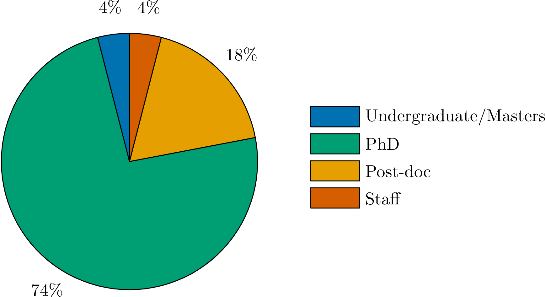
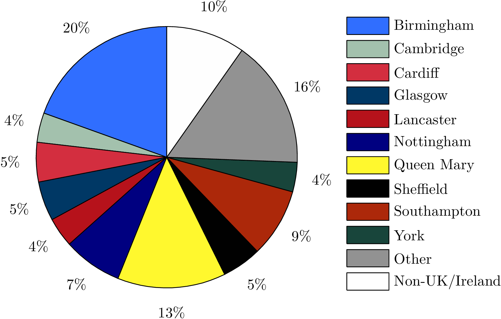
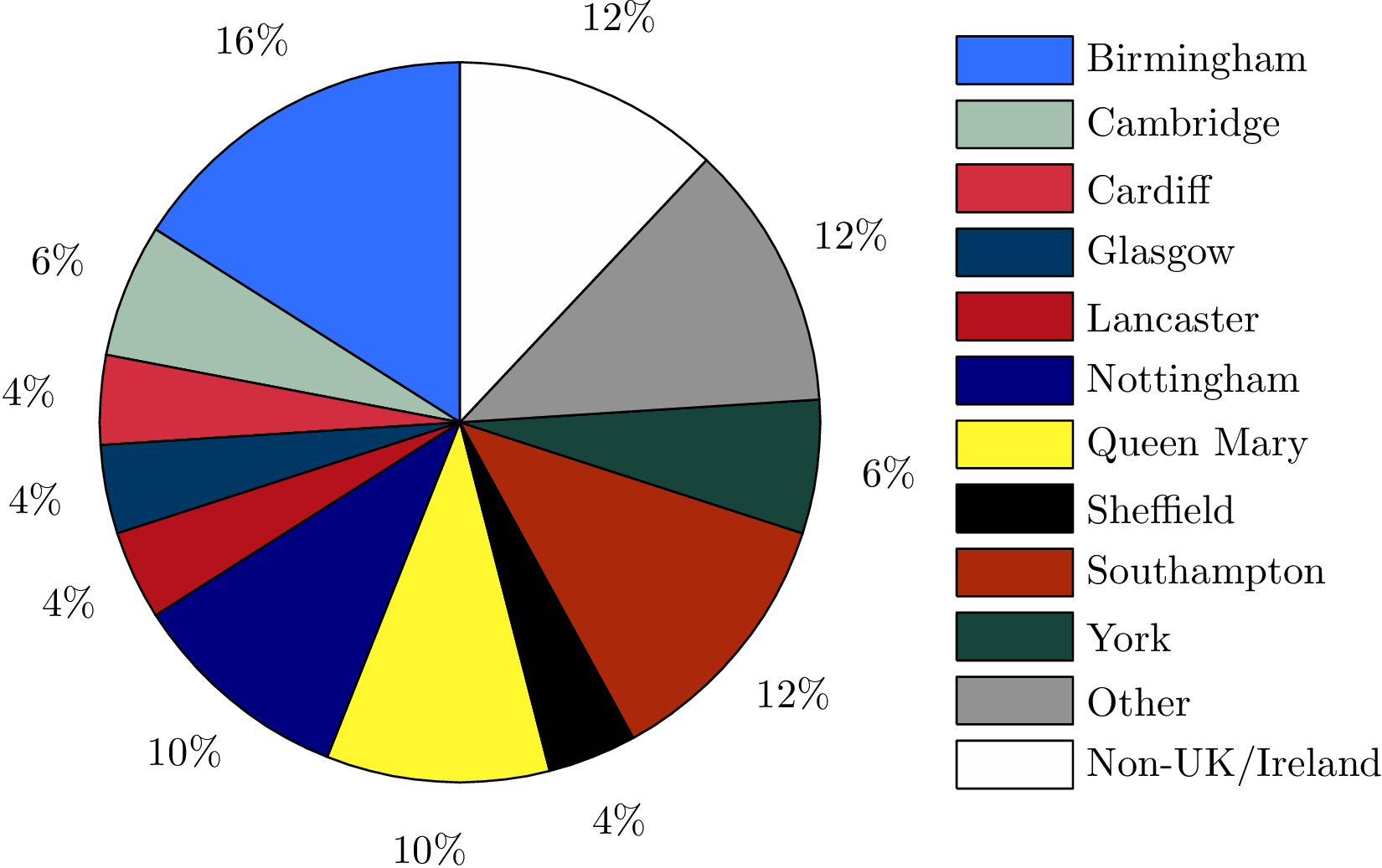
We had a fair amount of interest in the meeting. We totalled 81 (registered) participants at the meeting: a few more registered but didn’t make it in the end for various reasons and I suspect a couple of Birmingham people sneaked in without registering.
Looking at the attendance in more detail, we can break down the participants by their career-level. One of the aims of BritGrav is to showcase to research of early-career researchers (PhD students and post-docs), so we ask for this information on the registration form. The proportions are shown in the pie-chart below.
Proportion of participants at BritGrav 15 by (self-reported) career level.
PhD students make up the largest chunk; there are a few keen individuals who are yet to start a PhD, and a roughly even split between post-docs and permanent staff. We do need to encourage more senior researchers to come along, even if they are not giving talks, so that they can see the research done by others.
We had a total of 50 talks across the two days (including the two thesis-prize talks); the distribution of talks by career level as shown below.
Proportion of talks at BritGrav 15 by (self-reported) career level. The majority are by PhD students.
PhDs make up an even larger proportion of talks here, and we see that there are many more talks from post-docs than permanent staff members. This is exactly what we’re aiming for! For comparison, at the first BritGrav Meeting only 26% of talks were by PhD students, and 17% of talks were by post-docs. There’s been a radical change in the distribution of talks, shifting from senior to junior, although the contribution by post-docs ends up about the same.
We can also consider at the proportion of participants from different institutions, which is shown below.
Proportion of participants at BritGrav 15 by institution. Birmingham, as host, comes out top.
Here, any UK/Ireland institution which has one or no speakers is lumped together under “Other”, all these institutions had fewer than four participants. It’s good to see that we are attracting some international participants: of those from non-UK/Ireland institutions, two are from the USA and the rest are from Europe (France, Germany, The Netherlands and Slovenia). Birmingham makes up the largest chunk, which probably reflects the convenience. The list of top institutions closely resembles the list of institutions that have hosted a BritGrav. This could show that these are THE places for gravitational research in the UK, or possibly that the best advertising for future BritGravs is having been at an institution in the past (so everyone knows how awesome they are). The distribution of talks by institution roughly traces the number of participants, as shown below.
Proportion of talks at BritGrav 15 by institution.
Again Birmingham comes top, followed by Queen Mary and Southampton. Both of the thesis-prize talks were from people currently outside the UK/Ireland, even though they studied for their PhDs locally. I think we had a good mix of participants, which is one of factors that contributed to the meeting being successful.
I’m pleased with how well everything went at BritGrav 15, and now I’m looking forward to BritGrav 16, which I will not be organising.


![\displaystyle F_{ij} = \mu t_\mathrm{obs} \left[ \frac{1}{\mu^2} \frac{\partial \mu}{\partial \lambda_i} \frac{\partial \mu}{\partial \lambda_j} + \sum_k\frac{1}{p_k} \frac{\partial p_k}{\partial \lambda_i} \frac{\partial p_k}{\partial \lambda_j} \right]](https://s0.wp.com/latex.php?latex=%5Cdisplaystyle+F_%7Bij%7D+%3D+%5Cmu+t_%5Cmathrm%7Bobs%7D+%5Cleft%5B+%5Cfrac%7B1%7D%7B%5Cmu%5E2%7D+%5Cfrac%7B%5Cpartial+%5Cmu%7D%7B%5Cpartial+%5Clambda_i%7D%C2%A0%5Cfrac%7B%5Cpartial+%5Cmu%7D%7B%5Cpartial+%5Clambda_j%7D%C2%A0+%2B+%5Csum_k%5Cfrac%7B1%7D%7Bp_k%7D+%5Cfrac%7B%5Cpartial+p_k%7D%7B%5Cpartial+%5Clambda_i%7D%C2%A0%5Cfrac%7B%5Cpartial+p_k%7D%7B%5Cpartial+%5Clambda_j%7D+%5Cright%5D&bg=ffffff&fg=444444&s=0&c=20201002)


 , we want to know the probability that the parameters
  have different values, which is written as
  . This is calculated using
 ,
, is the likelihood, which we can calculate from our knowledge of the
  is the prior on the parameters (what we would have guessed before we had the data), and the normalisation constant
  is called the evidence. We’ll use the evidence again in the next layer of inference.
 ,
, denotes which model we are considering.
 , we can work this out using another application of Bayes’ theorem (yay)
 ,
, is just all the evidences for the individual events (given that model) multiplied together,
  is our prior for the different models, and
  is another normalisation constant.


 .
. and
and  (where
  is the mass of our Sun), and the final black hole was
  . The quoted values are the median values and the error bars denote the
 . The two-dimensional shows the probability distribution for GW170104 as well as 50% and 90% contours for all events. The one-dimensional plot shows results using different waveform models. The dotted lines mark the edge of our 90% probability intervals. Figure 2 of the
  . GW170104 has similar masses, showing that our first detection was not a fluke, but there really is a population of black holes with masses stretching up into this range.
 qualifies the impact of the spins on the rate of inspiral, and where the binary plunges together to merge. It ranges from +1, meaning both black holes are spinning as fast as possible and rotate in the same direction as the orbital motion, to −1, both black holes spinning as fast as possible but in the opposite direction to the way that the binary is orbiting. A value of 0 for
  qualifies the amount of precession, the way that the orbital plane and black hole
  . Therefore, we disfavour large spins aligned with the orbital angular momentum, but are consistent with small aligned spins, misaligned spins, or spins antialigned with the angular momentum. The value is similar to that for
  .
.

 . The spins of the component black holes are less significant, and can make it a bit higher of lower. We infer a final spin of
  ; there is a tail of lower spin values on account of the possibility that the two component black holes could be roughly antialigned with the orbital angular momentum.
 and spin
 for the final black hole. The two-dimensional shows the probability distribution for GW170104 as well as 50% and 90% contours. The one-dimensional plot shows results using different waveform models. The dotted lines mark the edge of our 90% probability intervals. Figure 6 of the GW170104 Supplemental Material (Figure 11 of the
  to
to  , and the uniform in log rate density goes from
  to
to  . The median values stay about the same, but the additional data have shrunk the uncertainties a little.
 at 90% probability. Figure 5 of the GW170104 Supplemental Material (Figure 10 of the
  .
.
 and binary inclination angle
  . The two-dimensional shows the probability distribution for GW170104 as well as 50% and 90% contours. The one-dimensional plot shows results using different waveform models. The dotted lines mark the edge of our 90% probability intervals. Figure 4 of the GW170104 Supplemental Material (Figure 9 of the
 (a much beloved combination of the two component masses which we are usually able to pin down precisely) and the total mass
  .
.
 is the mass of the stellar-mass black hole divided by the mass of the intermediate-mass black hole. Figure 1 of

 ). Figure 7 of