This paper, known as the Observing Scenarios Document with the Collaboration, outlines the observing plans of the ground-based detectors over the coming decade. If you want to search for electromagnetic or neutrino signals from our gravitational-wave sources, this is the paper for you. It is a living review—a document that is continuously updated.
This is the second published version, the big changes since the last version are
- We have now detected gravitational waves
- We have observed our first gravitational wave with a mulitmessenger counterpart [bonus note]
- We now include KAGRA, along with LIGO and Virgo
As you might imagine, these are quite significant updates! The first showed that we can do gravitational-wave astronomy. The second showed that we can do exactly the science this paper is about. The third makes this the first joint publication of the LIGO Scientific, Virgo and KAGRA Collaborations—hopefully the first of many to come.
I lead both this and the previous version. In my blog on the previous version, I explained how I got involved, and the long road that a collaboration must follow to get published. In this post, I’ll give an overview of the key details from the new version together with some behind-the-scenes background (working as part of a large scientific collaboration allows you to do amazing science, but it can also be exhausting). If you’d like a digest of this paper’s science, check out the LIGO science summary.
Commissioning and observing phases
The first section of the paper outlines the progression of detector sensitivities. The instruments are incredibly sensitive—we’ve never made machines to make these types of measurements before, so it takes a lot of work to get them to run smoothly. We can’t just switch them on and have them work at design sensitivity [bonus note].

Target evolution of the Advanced LIGO and Advanced Virgo detectors with time. The lower the sensitivity curve, the further away we can detect sources. The distances quoted are binary neutron star (BNS) ranges, the average distance we could detect a binary neutron star system. The BNS-optimized curve is a proposal to tweak the detectors for finding BNSs. Figure 1 of the Observing Scenarios Document.
The plots above show the planned progression of the different detectors. We had to get these agreed before we could write the later parts of the paper because the sensitivity of the detectors determines how many sources we will see and how well we will be able to localize them. I had anticipated that KAGRA would be the most challenging here, as we had not previously put together this sequence of curves. However, this was not the case, instead it was Virgo which was tricky. They had a problem with the silica fibres which suspended their mirrors (they snapped, which is definitely not what you want). The silica fibres were replaced with steel ones, but it wasn’t immediately clear what sensitivity they’d achieve and when. The final word was they’d observe in August 2017 and that their projections were unchanged. I was sceptical, but they did pull it out of the bag! We had our first clear three-detector observation of a gravitational wave 14 August 2017. Bravo Virgo!
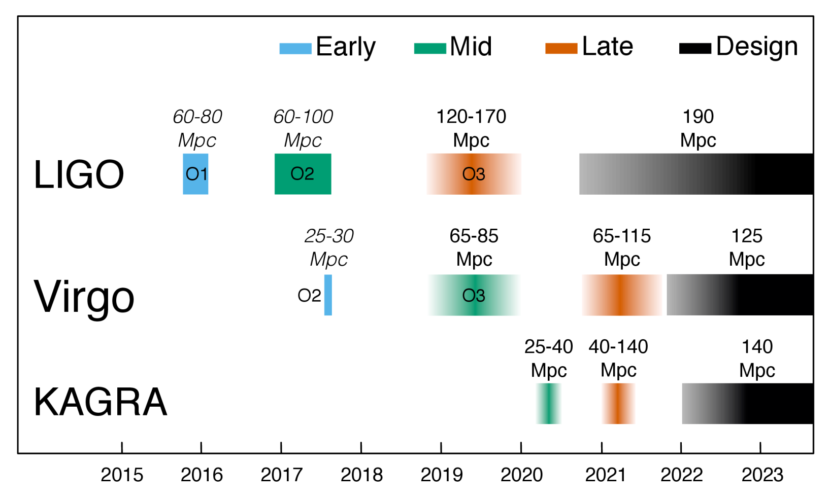
Plausible time line of observing runs with Advanced LIGO (Hanford and Livingston), advanced Virgo and KAGRA. It is too early to give a timeline for LIGO India. The numbers above the bars give binary neutron star ranges (italic for achieved, roman for target); the colours match those in the plot above. Currently our third observing run (O3) looks like it will start in early 2019; KAGRA might join with an early sensitivity run at the end of it. Figure 2 of the Observing Scenarios Document.
Searches for gravitational-wave transients
The second section explain our data analysis techniques: how we find signals in the data, how we work out probable source locations, and how we communicate these results with the broader astronomical community—from the start of our third observing run (O3), information will be shared publicly!
The information in this section hasn’t changed much [bonus note]. There is a nice collection of references on the follow-up of different events, including GW170817 (I’d recommend my blog for more on the electromagnetic story). The main update I wanted to include was information on the detection of our first gravitational waves. It turned out to be more difficult than I imagined to come up with a plot which showed results from the five different search algorithms (two which used templates, and three which did not) which found GW150914, and harder still to make a plot which everyone liked. This plot become somewhat infamous for the amount of discussion it generated. I think we ended up with something which was a good compromise and clearly shows our detections sticking out above the background of noise.
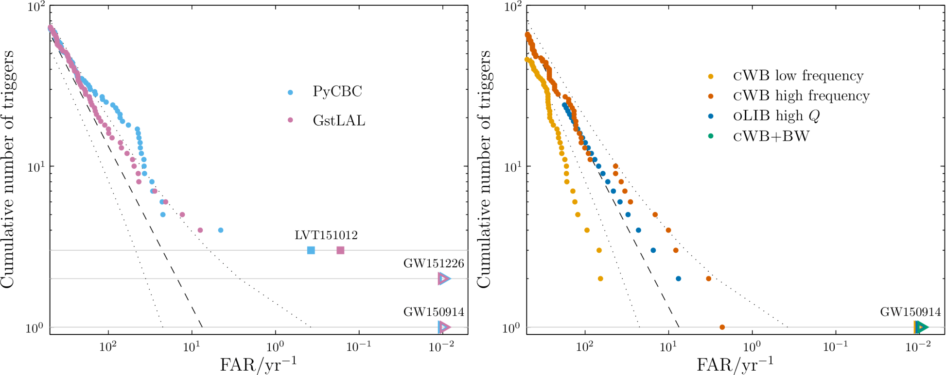
Offline transient search results from our first observing run (O1). The plot shows the number of events found verses false alarm rate: if there were no gravitational waves we would expect the points to follow the dashed line. The left panel shows the results of the templated search for compact binary coalescences (binary black holes, binary neutron stars and neutron star–black hole binaries), the right panel shows the unmodelled burst search. GW150914, GW151226 and LVT151012 are found by the templated search; GW150914 is also seen in the burst search. Arrows indicate bounds on the significance. Figure 3 of the Observing Scenarios Document.
Observing scenarios
The third section brings everything together and looks at what the prospects are for (gravitational-wave) multimessenger astronomy during each observing run. It’s really all about the big table.
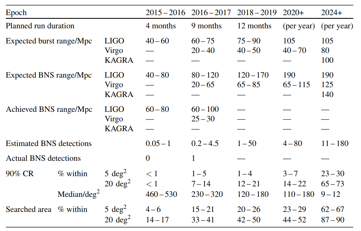
Summary of different observing scenarios with the advanced detectors. We assume a 70–75% duty factor for each instrument (including Virgo for the second scenario’s sky localization, even though it only joined our second observing run for the final month). Table 3 from the Observing Scenarios Document.
I think there are three really awesome take-aways from this
- Actual binary neutron stars detected = 1. We did it!
- Using the rates inferred using our observations so far (including GW170817), once we have the full five detector network of LIGO-Hanford, LIGO-Livingston, Virgo, KAGRA and LIGO-India, we could be detected 11–180 binary neutron stars a year. That something like between one a month to one every other day! I’m kind of scared…
- With the five detector network the sky localization is really good. The median localization is about 9–12 square degrees, about the area the LSST could cover in a single pointing! This really shows the benefit of adding more detector to the network. The improvement comes not because a source is much better localized with five detectors than four, but because when you have five detectors you almost always have at least three detectors(the number needed to get a good triangulation) online at any moment, so you get a nice localization for pretty much everything.
In summary, the prospects for observing and localizing gravitational-wave transients are pretty great. If you are an astronomer, make the most of the quiet before O3 begins next year.
arXiv: 1304.0670 [gr-qc]
Journal: Living Reviews In Relativity; 21:3(57); 2018
Science summary: A Bright today and brighter tomorrow: Prospects for gravitational-wave astronomy With Advanced LIGO, Advanced Virgo, and KAGRA
Prospects for the next update: After two updates, I’ve stepped down from preparing the next one. Wooh!
Bonus notes
GW170817 announcement
The announcement of our first multimessenger detection came between us submitting this update and us getting referee reports. We wanted an updated version of this paper, with the current details of our observing plans, to be available for our astronomer partners to be able to cite when writing their papers on GW170817.
Predictably, when the referee reports came back, we were told we really should include reference to GW170817. This type of discovery is exactly what this paper is about! There was avalanche of results surrounding GW170817, so I had to read through a lot of papers. The reference list swelled from 8 to 13 pages, but this effort was handy for my blog writing. After including all these new results, it really felt like this was version 2.5 of the Observing Scenarios, rather than version 2.
Design sensitivity
We use the term design sensitivity to indicate the performance the current detectors were designed to achieve. They are the targets we aim to achieve with Advanced LIGO, Advance Virgo and KAGRA. One thing I’ve had to try to train myself not to say is that design sensitivity is the final sensitivity of our detectors. Teams are currently working on plans for how we can upgrade our detectors beyond design sensitivity. Reaching design sensitivity will not be the end of our journey.
Binary black holes vs binary neutron stars
Our first gravitational-wave detections were from binary black holes. Therefore, when we were starting on this update there was a push to switch from focusing on binary neutron stars to binary black holes. I resisted on this, partially because I’m lazy, but mostly because I still thought that binary neutron stars were our best bet for multimessenger astronomy. This worked out nicely.

 as calculated by
  ,
, is the likelihood for data
  (the number of observations and their chirp mass distribution in our case),
  are our parameters (natal kick, etc.), and the angular brackets indicate the average over the population parameters. In statistics terminology, this is the variance of the
 , the common envelope efficiency
  , the Wolf–Rayet mass loss rate
  , and the luminous blue variable mass loss rate
  . There is an anticorrealtion between
  and
and 
 as following a Maxwell–Boltzmann distribution,
 ,
, is not the same as this, however, as we assume some of the material ejected by the supernova falls back, reducing the over kick. The final natal kick is
 ,
, is the fraction that falls back, taken from
  and the probability of falling in each chirp mass bin
  (we factor measurement uncertainty into this). Our observations are the the total number of detections
  and the number in each chirp mass bin
  (
( ). The likelihood is the probability of these observations given the model predictions. We can split the likelihood into two pieces, one for the rate, and one for the chirp mass distribution,
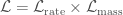 .
. ,
, is the total observing time. For the chirp mass likelihood, we the probability of getting a number of detections in each bin, given the predicted fractions. This is given by a
 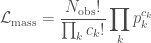 .
.![\displaystyle F_{ij} = \mu t_\mathrm{obs} \left[ \frac{1}{\mu^2} \frac{\partial \mu}{\partial \lambda_i} \frac{\partial \mu}{\partial \lambda_j} + \sum_k\frac{1}{p_k} \frac{\partial p_k}{\partial \lambda_i} \frac{\partial p_k}{\partial \lambda_j} \right]](https://s0.wp.com/latex.php?latex=%5Cdisplaystyle+F_%7Bij%7D+%3D+%5Cmu+t_%5Cmathrm%7Bobs%7D+%5Cleft%5B+%5Cfrac%7B1%7D%7B%5Cmu%5E2%7D+%5Cfrac%7B%5Cpartial+%5Cmu%7D%7B%5Cpartial+%5Clambda_i%7D%C2%A0%5Cfrac%7B%5Cpartial+%5Cmu%7D%7B%5Cpartial+%5Clambda_j%7D%C2%A0+%2B+%5Csum_k%5Cfrac%7B1%7D%7Bp_k%7D+%5Cfrac%7B%5Cpartial+p_k%7D%7B%5Cpartial+%5Clambda_i%7D%C2%A0%5Cfrac%7B%5Cpartial+p_k%7D%7B%5Cpartial+%5Clambda_j%7D+%5Cright%5D&bg=ffffff&fg=444444&s=0&c=20201002) .
. . Therefore, we can see that the measurement uncertainty defined by the inverse of the Fisher information matrix, scales on average as
  .
. and
and  are the same as their expectation values. The second-order derivatives are given by the expression we have worked out for the Fisher information matrix. Therefore, in the region around the maximum likelihood point, the Fisher information matrix encodes all the relevant information about the shape of the likelihood.
 , you’ll see that the distribution basically becomes a delta function at the maximum likelihood values. To check that our
  was large enough, we verified that higher-order derivatives were still small.