GW190425—First discovery from O3

January 6, 2020June 26, 2021 / CPLB / Leave a comment

The first gravitational wave detection of LIGO and Virgo’s third observing run (O3) has been announced: GW190425! [bonus note] The signal comes from the inspiral of two objects which have a combined mass of about 3.4 times the mass of our Sun. These masses are in range expected for neutron stars, this makes GW190425 the second observation of gravitational waves from a binary neutron star inspiral (after GW170817). While the individual masses of the two components agree with the masses of neutron stars found in binaries, the overall mass of the binary (times the mass of our Sun) is noticeably larger than any previously known binary neutron star system. GW190425 may be the first evidence for multiple ways of forming binary neutron stars.

The gravitational wave signal

On 25 April 2019 the LIGO–Virgo network observed a signal. This was promptly shared with the world as candidate event S190425z [bonus note]. The initial source classification was as a binary neutron star. This caused a flurry of excitement in the astronomical community [bonus note], as the smashing together of two neutron stars should lead to the emission of light. Unfortunately, the sky localization was HUGE (the initial 90% area wass about a quarter of the sky, and the refined localization provided the next day wasn’t much improvement), and the distance was four times that of GW170817 (meaning that any counterpart would be about 16 times fainter). Covering all this area is almost impossible. No convincing counterpart has been found [bonus note].

Early sky localization for GW190425. Darker areas are more probable. This localization was circulated in GCN 24228 on 26 April and was used to guide follow-up, even though it covers a huge amount of the sky (the 90% area is about 18% of the sky).

The localization for GW19045 was so large because LIGO Hanford (LHO) was offline at the time. Only LIGO Livingston (LLO) and Virgo were online. The Livingston detector was about 2.8 times more sensitive than Virgo, so pretty much all the information came from Livingston. I’m looking forward to when we have a larger network of detectors at comparable sensitivity online (we really need three detectors observing for a good localization).

We typically search for gravitational waves by looking for coincident signals in our detectors. When looking for binaries, we have templates for what the signals look like, so we match these to the data and look for good overlaps. The overlap is quantified by the signal-to-noise ratio. Since our detectors contains all sorts of noise, you’d expect them to randomly match templates from time to time. On average, you’d expect the signal-to-noise ratio to be about 1. The higher the signal-to-noise ratio, the less likely that a random noise fluctuation could account for this.

Our search algorithms don’t just rely on the signal-to-noise ratio. The complication is that there are frequently glitches in our detectors. Glitches can be extremely loud, and so can have a significant overlap with a template, even though they don’t look anything like one. Therefore, our search algorithms also look at the overlap for different parts of the template, to check that these match the expected distribution (for example, there’s not one bit which is really loud, while the others don’t match). Each of our different search algorithms has their own way of doing this, but they are largely based around the ideas from Allen (2005), which is pleasantly readable if you like these sort of things. It’s important to collect lots of data so that we know the expected distribution of signal-to-noise ratio and signal-consistency statistics (sometimes things change in our detectors and new types of noise pop up, which can confuse things).

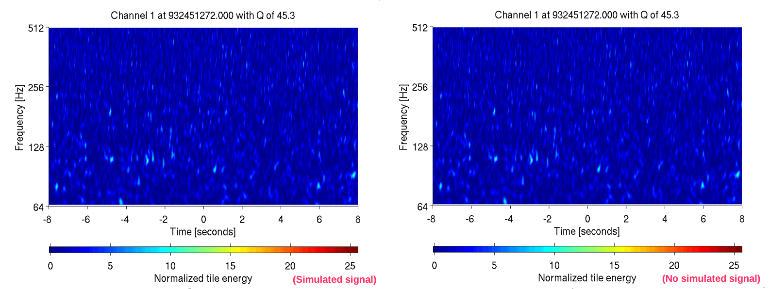
It is extremely important to check the state of the detectors at the time of an event candidate. In O3, we have unfortunately had to retract various candidate events after we’ve identified that our detectors were in a disturbed state. The signal consistency checks take care of most of the instances, but they are not perfect. Fortunately, it is usually easy to identify that there is a glitch—the difficult question is whether there is a glitch on top of a signal (as was the case for GW170817). Our checks revealed nothing up with the detectors which could explain the signal (there was a small glitch in Livingston about 60 seconds before the merger time, but this doesn’t overlap with the signal).

Now, the search that identified GW190425 was actually just looking for single-detector events: outliers in the distribution of signal-to-noise ratio and signal-consistency as expected for signals. This was a Good Thing™. While the signal-to-noise ratio in Livingston was 12.9 (pretty darn good), the signal-to-noise ration in Virgo was only 2.5 (pretty meh) [bonus note]. This is below the threshold (signal-to-noise ratio of 4) the search algorithms use to look for coincidences (a threshold is there to cut computational expense: the lower the threshold, the more triggers need to be checked) [bonus note]. The Bad Thing™ about GW190425 being found by the single-detector search, and being missed by the usual multiple detector search, is that it is much harder to estimate the false-alarm rate—it’s much harder to rule out the possibility of some unusual noise when you don’t have another detector to cross-reference against. We don’t have a final estimate for the significance yet. The initial estimate was 1 in 69,000 years (which relies on significant extrapolation). What we can be certain of is that this event is a noticeable outlier: across the whole of O1, O2 and the first 50 days of O3, it comes second only to GW170817. In short, we can say that GW190425 is worth betting on, but I’m not sure (yet) how heavily you want to bet.

Comparison of GW190425 to O1, O2 and start of O3 data

Detection statistics for GW190425 showing how it stands out from the background. The left plot shows the signal-to-noise ratio (SNR) and signal-consistency statistic from the GstLAL algorithm, which made the detection. The coloured density plot shows the distribution of background triggers. Right shows the detection statistic from PyCBC, which combines the SNR and their signal-consistency statistic. The lines show the background distributions. GW190425 is more significant than everything apart from GW170817. Adapted from Figures 1 and 6 of the GW190425 Discovery Paper.

I’m always cautious of single-detector candidates. If you find a high-mass binary black hole (which would be an extremely short template), or something with extremely high spins (indicating that the templates don’t match unless you push to the bounds of what is physical), I would be suspicious. Here, we do have consistent Virgo data, which is good for backing up what is observed in Livingston. It may be a single-detector detection, but it is a multiple-detector observation. To further reassure ourselves about GW190425, we ran our full set of detection algorithms on the Livingston data to check that they all find similar signals, with reasonable signal-consistency test values. Indeed, they do! The best explanation for the data seems to be a gravitational wave.

The source

Given that we have a gravitational wave, where did it come from? The best-measured property of a binary inspiral is its chirp mass—a particular combination of the two component masses. For GW190425, this is $1.44^{+0.02}_{-0.02}$ solar masses (quoting the 90% range for parameters). This is larger than GW170817’s $1.186^{+0.001}_{-0.001}$ solar masses: we have a heavier binary.

Estimated masses for the two components in the binary. We show results for two different spin limits. The two-dimensional shows the 90% probability contour, which follows a line of constant chirp mass. The one-dimensional plot shows individual masses; the dotted lines mark 90% bounds away from equal mass. The masses are in the range expected for neutron stars. Figure 3 of the GW190425 Discovery Paper.

Figuring out the component masses is trickier. There is a degeneracy between the spins and the mass ratio—by increasing the spins of the components it is possible to get more extreme mass ratios to fit the signal. As we did for GW170817, we quote results with two ranges of spins. The low-spin results use a maximum spin of 0.05, which matches the range of spins we see for binary neutron stars in our Galaxy, while the high-spin results use a limit of 0.89, which safely encompasses the upper limit for neutron stars (if they spin faster than about 0.7 they’ll tear themselves apart). We find that the heavier component of the binary has a mass of $1.62$ – $1.88$ solar masses with the low-spin assumption, and $1.61$ – $2.52$ solar masses with the high-spin assumption; the lighter component has a mass $1.45$ – $1.69$ solar masses with the low-spin assumption, and $1.12$ – $1.68$ solar masses with the high-spin. These are the range of masses expected for neutron stars.

Without an electromagnetic counterpart, we cannot be certain that we have two neutron stars. We could tell from the gravitational wave by measuring the imprint in the signal left by the tidal distortion of the neutron star. Black holes have a tidal deformability of 0, so measuring a nonzero tidal deformability would be the smoking gun that we have a neutron star. Unfortunately, the signal isn’t loud enough to find any evidence of these effects. This isn’t surprising—we couldn’t say anything for GW170817, without assuming its source was a binary neutron star, and GW170817 was louder and had a lower mass source (where tidal effects are easier to measure). We did check—it’s probably not the case that the components were made of marshmallow, but there’s not much more we can say (although we can still make pretty simulations). It would be really odd to have black holes this small, but we can’t rule out than at least one of the components was a black hole.

Two binary neutron stars is the most likely explanation for GW190425. How does it compare to other binary neutron stars? Looking at the 17 known binary neutron stars in our Galaxy, we see that GW190425’s source is much heavier. This is intriguing—could there be a different, previously unknown formation mechanism for this binary? Perhaps the survey of Galactic binary neutron stars (thanks to radio observations) is incomplete? Maybe the more massive binaries form in close binaries, which are had to spot in the radio (as the neutron star moves so quickly, the radio signals gets smeared out), or maybe such heavy binaries only form from stars with low metallicity (few elements heavier than hydrogen and helium) from earlier in the Universe’s history, so that they are no longer emitting in the radio today? I think it’s too early to tell—but it’s still fun to speculate. I expect there’ll be a flurry of explanations out soon.

Galactic binary neutron stars and GW190425

Comparison of the total binary mass of the 10 known binary neutron stars in our Galaxy that will merge within a Hubble time and GW190425’s source (with both the high-spin and low-spin assumptions). We also show a Gaussian fit to the Galactic binaries. GW190425’s source is higher mass than previously known binary neutron stars. Figure 5 of the GW190425 Discovery Paper.

Since the source seems to be an outlier in terms of mass compared to the Galactic population, I’m a little cautious about using the low-spin results—if this sample doesn’t reflect the full range of masses, perhaps it doesn’t reflect the full range of spins too? I think it’s good to keep an open mind. The fastest spinning neutron star we know of has a spin of around 0.4, maybe binary neutron star components can spin this fast in binaries too?

One thing we can measure is the distance to the source: $160^{+70}_{-70}~\mathrm{Mpc}$ . That means the signal was travelling across the Universe for about half a billion years. This is as many times bigger than diameter of Earth’s orbit about the Sun, as the diameter of the orbit is than the height of a LEGO brick. Space is big.

We have now observed two gravitational wave signals from binary neutron stars. What does the new observation mean for the merger rate of binary neutron stars? To go from an observed number of signals to how many binaries are out there in the Universe we need to know how sensitive our detectors are to the sources. This depends on the masses of the sources, since more massive binaries produce louder signals. We’re not sure of the mass distribution for binary neutron stars yet. If we assume a uniform mass distribution for neutron stars between 0.8 and 2.3 solar masses, then at the end of O2 we estimated a merger rate of $110$ – $2520~\mathrm{Gpc^{-3}\,\mathrm{yr}^{-3}}$ . Now, adding in the first 50 days of O3, we estimate the rate to be $250$ – $2470~\mathrm{Gpc^{-3}\,\mathrm{yr}^{-3}}$ , so roughly the same (which is nice) [bonus note].

Since GW190425’s source looks rather different from other neutron stars, you might be interested in breaking up the merger rates to look at different classes. Using measured masses, we can construct rates for GW170817-like (matching the usual binary neutron star population) and GW190425-like binaries (we did something similar for binary black holes after our first detection). The GW170817-like rate is $110$ – $2500~\mathrm{Gpc^{-3}\,\mathrm{yr}^{-3}}$ , and the GW190425-like rate is lower at $70$ – $4600~\mathrm{Gpc^{-3}\,\mathrm{yr}^{-3}}$ . Combining the two (Assuming that binary neutron stars are all one class or the other), gives an overall rate of $290$ – $2810~\mathrm{Gpc^{-3}\,\mathrm{yr}^{-3}}$ , which is not too different than assuming the uniform distribution of masses.

Given these rates, we might expect some more nice binary neutron star signals in the O3 data. There is a lot of science to come.

Future mysteries

GW190425 hints that there might be a greater variety of binary neutron stars out there than previously thought. As we collect more detections, we can start to reconstruct the mass distribution. Using this, together with the merger rate, we can start to pin down the details of how these binaries form.

As we find more signals, we should also find a few which are loud enough to measure tidal effects. With these, we can start to figure out the properties of the Stuff™ which makes up neutron stars, and potentially figure out if there are small black holes in this mass range. Discovering smaller black holes would be extremely exciting—these wouldn’t be formed from collapsing stars, but potentially could be remnants left over from the early Universe.

Neutron star masses and radii for GW190425

Probability distributions for neutron star masses and radii (blue for the more massive neutron star, orange for the lighter), assuming that GW190425’s source is a binary neutron star. The left plots use the high-spin assumption, the right plots use the low-spin assumptions. The top plots use equation-of-state insensitive relations, and the bottom use parametrised equation-of-state models incorporating the requirement that neutron stars can be 1.97 solar masses. Similar analyses were done in the GW170817 Equation-of-state Paper. In the one-dimensional plots, the dashed lines indicate the priors. Figure 16 of the GW190425 Discovery Paper.

With more detections (especially when we have more detectors online), we should also be lucky enough to have a few which are well localised. These are the events when we are most likely to find an electromagnetic counterpart. As our gravitational-wave detectors become more sensitive, we can detect sources further out. These are much harder to find counterparts for, so we mustn’t expect every detection to have a counterpart. However, for nearby sources, we will be able to localise them better, and so increase our odds of finding a counterpart. From such multimessenger observations we can learn a lot. I’m especially interested to see how typical GW170817 really was.

O3 might see gravitational wave detection becoming routine, but that doesn’t mean gravitational wave astronomy is any less exciting!

Title: GW190425: Observation of a compact binary coalescence with total mass ~ 3.4 solar masses
Journal: Astrophysical Journal Letters; 892(1):L3(24); 2020
arXiv: arXiv:2001.01761 [astro-ph.HE] [bonus note]
Science summary: GW190425: The heaviest binary neutron star system ever seen?
Data release: Gravitational Wave Open Science Center; Parameter estimation results
Rating: 🥇😮🥂🥇

Bonus notes

Exceptional events

The plan for publishing papers in O3 is that we would write a paper for any particularly exciting detections (such as a binary neutron star), and then put out a catalogue of all our results later. The initial discovery papers wouldn’t be the full picture, just the key details so that the entire community could get working on them. Our initial timeline was to get the individual papers out in four months—that’s not going so well, it turns out that the most interesting events have lots of interesting properties, which take some time to understand. Who’d have guessed?

We’re still working on getting papers out as soon as possible. We’ll be including full analyses, including results which we can’t do on these shorter timescales in our catalogue papers. The catalogue paper for the first half of O3 (O3a) is currently pencilled in for April 2020.

Naming conventions

The name of a gravitational wave signal is set by the date it is observed. GW190425 is hence the gravitational wave (GW) observed on 2019 April 25th. Our candidates alerts don’t start out with the GW prefix, as we still need to do lots of work to check if they are real. Their names start with S for superevent (not for hope) [bonus bonus note], then the date, and then a letter indicating the order it was uploaded to our database of candidates (we upload candidates with false alarm rates of around one per hour, so there are multiple database entries per day, and most are false alarms). S190425z was the 26th superevent uploaded on 2019 April 25th.

What is a superevent? We call anything flagged by our detection pipelines an event. We have multiple detection pipelines, and often multiple pipelines produce events for the same stretch of data (you’d expect this to happen for real signals). It was rather confusing having multiple events for the same signal (especially when trying to quickly check a candidate to issue an alert), so in O3 we group together events from similar times into SUPERevents.

GRB 190425?

Pozanenko et al. (2019) suggest a gamma-ray burst observed by INTEGRAL (first reported in GCN 24170). The INTEGRAL team themselves don’t find anything in their data, and seem sceptical of the significance of the detection claim. The significance of the claim seems to be based on there being two peaks in the data (one about 0.5 seconds after the merger, one 5.9 seconds after the merger), but I’m not convinced why this should be the case. Nothing was observed by Fermi, which is possibly because the source was obscured by the Earth for them. I’m interested in seeing more study of this possible gamma-ray burst.

EMMA 2019

At the time of GW190425, I was attending the first day of the Enabling Multi-Messenger Astrophysics in the Big Data Era Workshop. This was a meeting bringing together many involved in the search for counterparts to gravitational wave events. The alert for S190425z cause some excitement. I don’t think there was much sleep that week.

The cafeteria at @stsci is just a war room now, with people scheduling satellites and telescopes all over the world, on the phone with colleagues, running around sharing rumors and the latest info. Exciting! @LIGO #Emma2019 pic.twitter.com/2BnvOtYNcJ

— Andy Howell (@d_a_howell) April 26, 2019

Signal-to-noise ratio ratios

The signal-to-noise ratio reported from our search algorithm for LIGO Livingston is 12.9, and the same code gives 2.5 for Virgo. Virgo was about 2.8 times less sensitive that Livingston at the time, so you might be wondering why we have a signal-to-noise ratio of 2.8, instead of 4.6? The reason is that our detectors are not equally sensitive in all directions. They are most sensitive directly to sources directly above and below, and less sensitive to sources from the sides. The relative signal-to-noise ratios, together with the time or arrival at the different detectors, helps us to figure out the directions the signal comes from.

Detection thresholds

In O2, GW170818 was only detected by GstLAL because its signal-to-noise ratios in Hanford and Virgo (4.1 and 4.2 respectively) were below the threshold used by PyCBC for their analysis (in O2 it was 5.5). Subsequently, PyCBC has been rerun on the O2 data to produce the second Open Gravitational-wave Catalog (2-OGC). This is an analysis performed by PyCBC experts both inside and outside the LIGO Scientific & Virgo Collaboration. For this, a threshold of 4 was used, and consequently they found GW170818, which is nice.

I expect that if the threshold for our usual multiple-detector detection pipelines were lowered to ~2, they would find GW190425. Doing so would make the analysis much trickier, so I’m not sure if anyone will ever attempt this. Let’s see. Perhaps the 3-OGC team will be feeling ambitious?

Rates calculations

In comparing rates calculated for this papers and those from our end-of-O2 paper, my student Chase Kimball (who calculated the new numbers) would like me to remember that it’s not exactly an apples-to-apples comparison. The older numbers evaluated our sensitivity to gravitational waves by doing a large number of injections: we simulated signals in our data and saw what fraction of search algorithms could pick out. The newer numbers used an approximation (using a simple signal-to-noise ratio threshold) to estimate our sensitivity. Performing injections is computationally expensive, so we’re saving that for our end-of-run papers. Given that we currently have only two detections, the uncertainty on the rates is large, and so we don’t need to worry too much about the details of calculating the sensitivity. We did calibrate our approximation to past injection results, so I think it’s really an apples-to-pears-carved-into-the-shape-of-apples comparison.

Paper release

The original plan for GW190425 was to have the paper published before the announcement, as we did with our early detections. The timeline neatly aligned with the AAS meeting, so that seemed like an good place to make the announcement. We managed to get the the paper submitted, and referee reports back, but we didn’t quite get everything done in time for the AAS announcement, so Plan B was to have the paper appear on the arXiv just after the announcement. Unfortunately, there was a problem uploading files to the arXiv (too large), and by the time that was fixed the posting deadline had passed. Therefore, we went with Plan C or sharing the paper on the LIGO DCC. Next time you’re struggling to upload something online, remember that it happens to Nobel-Prize winning scientific collaborations too.

On the question of when it is best to share a paper, I’m still not decided. I like the idea of being peer-reviewed before making a big splash in the media. I think it is important to show that science works by having lots of people study a topic, before coming to a consensus. Evidence needs to be evaluated by independent experts. On the other hand, engaging the entire community can lead to greater insights than a couple of journal reviewers, and posting to arXiv gives opportunity to make adjustments before you having the finished article.

I think I am leaning towards early posting in general—the amount of internal review that our Collaboration papers receive, satisfies my requirements that scientists are seen to be careful, and I like getting a wider range of comments—I think this leads to having the best paper in the end.

S

The joke that S stands for super, not hope is recycled from an article I wrote for the LIGO Magazine. The editor, Hannah Middleton wasn’t sure that many people would get the reference, but graciously printed it anyway. Did people get it, or do I need to fly around the world really fast?

Top 2016 gravitational wave papers

January 14, 2017March 21, 2020 / CPLB / 2 Comments

2016 was a busy year for gravitational-wave astronomy. I wrote many blog posts about the papers I have been involved with (I still have a back log). Therefore, as a change, I thought I’d start 2017 looking at my favourite papers written by other people published in 2016. Here are my top three.

Prospects for multiband gravitational-wave astronomy after GW150914

Author: Sesana, A.
arXiv: 1602.06951 [gr-qc]
Journal: Physical Review Letters; 116(23):231102(6); 2016

I wrote about this paper previously when discussing the papers released to coincide the the announcement of the observation of GW150914. It suggests that we will be able to observe binary black holes months to years before they’re detectable with ground-based detectors with a space-borne detector like LISA. With this multi-band gravitational-wave astronomy, we could be able to learn even more about black holes

The concept of multi-band gravitational-wave astronomy is not actually new. I believe it was first suggested for LIGO and LISA detecting intermediate-mass black hole binaries (binaries with black holes about 100 times the mass of our Sun); it has also been suggested for combining LISA and pulsar timing measurements to look at supermassive black hole binaries (tens of millions to billions of times the mass of our Sun). However, this paper was to first to look at what we could really learn from these observations. We should be able to get a good sky localization (less than a square degree) ahead of the merger, meaning we can point telescopes ahead of time to try to catch any flash that might accompany it; we’ll also know when the merger should happen, so that we don’t need to worry about misidentifying any explosions we might spot. LISA would be able to provide good constraints of the black hole masses, measuring the chirp mass to an accuracy of less than 0.01%!

This paper created some real enthusiasm for multi-band gravitational-wave astronomy. Vitale (2016) considered how the combined measurements could help us test general relativity. Breivik et al. (2016) and Nishizawa et al. (2106) looked at how LISA could measure the eccentricity of these binaries (which is practically impossible by the time they are observable with ground-based detectors) to figure out how they form. I think these will be fruitful avenues of research in the future.

The excitement surrounding LISA is well timed. A mission proposal has just been submitted to ESA for their upcoming Gravitational Universe science theme. NASA has also stated interest in rejoining the mission.

Astrophysical constraints on massive black hole binary evolution from pulsar timing arrays

Authors: Middleton, H.; Del Pozzo, W.; Farr, W.M.; Sesana, A. & Vecchio, A.
arXiv: 1507.00992 [astro-ph.CO]
Journal: Monthly Notices of the Royal Astronomical Society Letters; 455(1):L72–L76; 2016

This is a really neat paper studying what we could learn form pulsar timing arrays. Pulsar timing arrays are sensitive to very low frequency gravitational waves, those from supermassive black hole binaries (millions to billions the times the mass of our Sun). Lots of work has been invested in trying to detect a signal. There are three consortia currently working towards this, collaborating together as part of the International Pulsar Timing Array , but I suspect secretly hoping that they can get there first. This papers looks at what we’ll actually be able to infer about the supermassive black holes when we do make a detection.

They find, unsurprisingly, that using our current upper limits on the background of gravitational waves, we can place some constraints on the number of mergers, but not say much else. If the upper limit was to improve by an order of magnitude, we’d start to learn something about the mass distribution but we wouldn’t learn much about the shape. When we do make a detection, we get more information, but still not a lot. We would know that some binaries are merging, but not which ones: there are degeneracies between the merger rate and the mass distribution. This means that even with a detection, pulsar timing will not be able to pin down the distribution of supermassive black holes, we’ll have to fold in other observations too!

Gravitational waves might be cool, but they can’t tell us everything.

Theoretical physics implications of the binary black-hole mergers GW150914 and GW151226

Authors: Yunes, N.; Yagi, K. & Pretorius, F.
arXiv: 1603.08955 [gr-qc]
Journal: Physical Review D; 94(8):084002(42); 2016

After a LISA paper and a pulsar-timing array paper, we’ll round off the trio with a LIGO paper. This paper takes an exhaustive view of the all the ways that the observations of gravitational-wave events so far constrain theories of gravity. It’s an impressive work, made even more so considering that they revised the paper following the announcement of GW151226. I would have been tempted to write a second paper on that. At 42 pages, this is heavy ready (it’s the least fun of my top 3), so it is perhaps best just to dip in to find out about your favourite alternative theories of gravity.

This paper highlights how the first observations of gravitational waves change the game when it comes to testing gravity. We now have a wealth of information on gravitational-wave generation, gravitational-wave propagation and the structure of black holes. This is great for cutting down the range of possible theories. However, as the authors point out, to really test other theories of gravity, we need predictions for their behaviour in the extreme and dynamic conditions of a binary black hole coalescence. There is still a huge amount of work to do.

I especially like this paper as it is an example of how results from LIGO and Virgo can be taken forward and put to good use by those outside of the Collaboration. I hope there will be more of this in the future.

Parameter estimation on gravitational waves from neutron-star binaries with spinning components

October 1, 2016October 15, 2017 / CPLB / Leave a comment

blIn gravitation-wave astronomy, some parameters are easier to measure than others. We are sensitive to properties which change the form of the wave, but sometimes the effect of changing one parameter can be compensated by changing another. We call this a degeneracy. In signals for coalescing binaries (two black holes or neutron stars inspiralling together), there is a degeneracy between between the masses and spins. In this recently published paper, we look at what this means for observing binary neutron star systems.

History

This paper has been something of an albatross, and I’m extremely pleased that we finally got it published. I started working on it when I began my post-doc at Birmingham in 2013. Back then I was sharing an office with Ben Farr, and together with others in the Parameter Estimation Group, we were thinking about the prospect of observing binary neutron star signals (which we naively thought were the most likely) in LIGO’s first observing run.

One reason that this work took so long is that binary neutron star signals can be computationally expensive to analyse [bonus note]. The signal slowly chirps up in frequency, and can take up to a minute to sweep through the range of frequencies LIGO is sensitive to. That gives us a lot of gravitational wave to analyse. (For comparison, GW150914 lasted 0.2 seconds). We need to calculate waveforms to match to the observed signals, and these can be especially complicated when accounting for the effects of spin.

A second reason is shortly after submitting the paper in August 2015, we got a little distracted…

This paper was the third of a trilogy look at measuring the properties of binary neutron stars. I’ve written about the previous instalment before. We knew that getting the final results for binary neutron stars, including all the important effects like spin, would take a long time, so we planned to follow up any detections in stages. A probable sky location can be computed quickly, then we can have a first try at estimating other parameters like masses using waveforms that don’t include spin, then we go for the full results with spin. The quicker results would be useful for astronomers trying to find any explosions that coincided with the merger of the two neutron stars. The first two papers looked at results from the quicker analyses (especially at sky localization); in this one we check what effect neglecting spin has on measurements.

What we did

We analysed a population of 250 binary neutron star signals (these are the same as the ones used in the first paper of the trilogy). We used what was our best guess for the sensitivity of the two LIGO detectors in the first observing run (which was about right).

The simulated neutron stars all have small spins of less than 0.05 (where 0 is no spin, and 1 would be the maximum spin of a black hole). We expect neutron stars in these binaries to have spins of about this range. The maximum observed spin (for a neutron star not in a binary neutron star system) is around 0.4, and we think neutron stars should break apart for spins of 0.7. However, since we want to keep an open mind regarding neutron stars, when measuring spins we considered spins all the way up to 1.

What we found

Our results clearly showed the effect of the mass–spin degeneracy. The degeneracy increases the uncertainty for both the spins and the masses.

Even though the true spins are low, we find that across the 250 events, the median 90% upper limit on the spin of the more massive (primary) neutron star is 0.70, and the 90% limit on the less massive (secondary) neutron star is 0.86. We learn practically nothing about the spin of the secondary, but a little more about the spin of the primary, which is more important for the inspiral. Measuring spins is hard.

The effect of the mass–spin degeneracy for mass measurements is shown in the plot below. Here we show a random selection of events. The banana-shaped curves are the 90% probability intervals. They are narrow because we can measure a particular combination of masses, the chirp mass, really well. The mass–spin degeneracy determines how long the banana is. If we restrict the range of spins, we explore less of the banana (and potentially introduce an offset in our results).

Rough outlines for 90% credible regions for component masses for a random assortments of signals. The circles show the true values. The coloured lines indicate the extent of the distribution with different limits on the spins. The grey area is excluded from our convention on masses $m_1 \geq m_2$ . Figure 5 from Farr et al. (2016).

Although you can’t see it in the plot above, including spin does also increase the uncertainty in the chirp mass too. The plots below show the standard deviation (a measure width of the posterior probability distribution), divided by the mean for several mass parameters. This gives a measure of the fractional uncertainty in our measurements. We show the chirp mass $\mathcal{M}_\mathrm{c}$ , the mass ratio $q = m_2/m_1$ and the total mass $M = m_1 + m_2$ , where $m_1$ and $m_2$ are the masses of the primary and secondary neutron stars respectively. The uncertainties are small for louder signals (higher signal-to-noise ratio). If we neglect the spin, the true chirp mass can lie outside the posterior distribution, the average is about 5 standard deviations from the mean, but if we include spin, the offset is just 0.7 from the mean (there’s still some offset as we’re allowing for spins all the way up to 1).

Mass measurements for binary neutron stars with and without spin

Fractional statistical uncertainties in chirp mass (top), mass ratio (middle) and total mass (bottom) estimates as a function of network signal-to-noise ratio for both the fully spinning analysis and the quicker non-spinning analysis. The lines indicate approximate power-law trends to guide the eye. Figure 2 of Farr et al. (2016).

We need to allow for spins when measuring binary neutron star masses in order to explore for the possible range of masses.

Sky localization and distance, however, are not affected by the spins here. This might not be the case for sources which are more rapidly spinning, but assuming that binary neutron stars do have low spin, we are safe using the easier-to-calculate results. This is good news for astronomers who need to know promptly where to look for explosions.

arXiv: 1508.05336 [astro-ph.HE]
Journal: Astrophysical Journal; 825(2):116(10); 2016
Authorea [bonus note]: Parameter estimation on gravitational waves from neutron-star binaries with spinning components
Conference proceedings: Early Advanced LIGO binary neutron-star sky localization and parameter estimation
Favourite albatross: Wilbur

Bonus notes

How long?

The plot below shows how long it took to analyse each of the binary neutron star signals.

Run time for different analyses of binary neutron stars

Distribution of run times for binary neutron star signals. Low-latency sky localization is done with BAYESTAR; medium-latency non-spinning parameter estimation is done with LALInference and TaylorF2 waveforms, and high-latency fully spinning parameter estimation is done with LALInference and SpinTaylorT4 waveforms. The LALInference results are for 2000 posterior samples. Figure 9 from Farr et al. (2016).

BAYESTAR provides a rapid sky localization, taking less than ten seconds. This is handy for astronomers who want to catch a flash caused by the merger before it fades.

Estimates for the other parameters are computed with LALInference. How long this takes to run depends on which waveform you are using and how many samples from the posterior probability distribution you want (the more you have, the better you can map out the shape of the distribution). Here we show times for 2000 samples, which is enough to get a rough idea (we collected ten times more for GW150914 and friends). Collecting twice as many samples takes (roughly) twice as long. Prompt results can be obtained with a waveform that doesn’t include spin (TaylorF2), these take about a day at most.

For this work, we considered results using a waveform which included the full effects of spin (SpinTaylorT4). These take about twenty times longer than the non-spinning analyses. The maximum time was 172 days. I have a strong suspicion that the computing time cost more than my salary.

Waiting for LALInference runs to finish gives you some time to practise hobbies. This is a globe knitted by Hannah. The two LIGO sites marked in red, and a typical gravitational-wave sky localization stitched on.

In order to get these results, we had to add check-pointing to our code, so we could stop it and restart it; we encountered a new type of error in the software which manages jobs running on our clusters, and Hannah Middleton and I got several angry emails from cluster admins (who are wonderful people) for having too many jobs running.

In comparison, analysing GW150914, LVT151012 and GW151226 was a breeze. Grudgingly, I have to admit that getting everything sorted out for this study made us reasonably well prepared for the real thing. Although, I’m not looking forward to that first binary neutron star signal…

Authorea

Authorea is an online collaborative writing service. It allows people to work together on documents, editing text, adding comments, and chatting with each other. By the time we came to write up the paper, Ben was no longer in Birmingham, and many of our coauthors are scattered across the globe. Ben thought Authorea might be useful for putting together the paper.

Writing was easy, and the ability to add comments on the text was handy for getting feedback from coauthors. The chat was going for quickly sorting out issues like plots. Overall, I was quite pleased, up to the point we wanted to get the final document. Extracted a nicely formatted PDF was awkward. For this I switched to using the Github back-end. On reflection, a simple git repo, plus a couple of Skype calls might have been a smoother way of writing, at least for a standard journal article.

Authorea promises to be an open way of producing documents, and allows for others to comment on papers. I don’t know if anyone’s looked at our Authorea article. For astrophysics, most people use the arXiv, which is free to everyone, and I’m not sure if there’s enough appetite for interaction (beyond the occasional email to authors) to motivate people to look elsewhere. At least, not yet.

In conclusion, I think Authorea is a nice idea, and I would try out similar collaborative online writing tools again, but I don’t think I can give it a strong recommendation for your next paper unless you have a particular idea in mind of how to make the most of it.

The Boxing Day Event

June 15, 2016February 8, 2020 / CPLB / 2 Comments

Advanced LIGO’s first observing run (O1) got off to an auspicious start with the detection of GW150914 (The Event to its friends). O1 was originally planned to be three months long (September to December), but after the first discovery, there were discussions about extending the run. No major upgrades to the detectors were going to be done over the holidays anyway, so it was decided that we might as well leave them running until January.

By the time the Christmas holidays came around, I was looking forward to some time off. And, of course, lots of good food and the Doctor Who Christmas Special. The work on the first detection had been exhausting, and the Collaboration reached the collective decision that we should all take some time off [bonus note]. Not a creature was stirring, not even a mouse.

On Boxing Day, there was a sudden flurry of emails. This could only mean one thing. We had another detection! Merry GW151226 [bonus note]!

I assume someone left out milk and cookies at the observatories. A not too subtle hint from Nutsinee Kijbunchoo’s comic in the LIGO Magazine.

I will always be amazed how lucky we were detecting GW150914. This could have been easily missed if we were just a little later starting observing. If that had happened, we might not have considered extended O1, and would have missed GW151226 too!

GW151226 is another signal from a binary black hole coalescence. This wasn’t too surprising at the time, as we had estimated such signals should be pretty common. It did, however, cause a slight wrinkle in discussions of what to do in the papers about the discovery of GW150914. Should we mention that we had another potential candidate? Should we wait until we had analysed the whole of O1 fully? Should we pack it all in and have another slice of cake? In the end we decided that we shouldn’t delay the first announcement, and we definitely shouldn’t rush the analysis of the full data set. Therefore, we went ahead with the original plan of just writing about the first month of observations and giving slightly awkward answers, mumbling about still having data to analyse, when asked if we had seen anything else [bonus note]. I’m not sure how many people outside the Collaboration suspected.

The science

What have we learnt from analysing GW151226, and what have we learnt from the whole of O1? We’ve split our results into two papers.

0. The Boxing Day Discovery Paper

Title: GW151226: Observation of gravitational waves from a 22-solar-mass binary black hole
arXiv: 1606.04855 [gr-qc]
Journal: Physical Review Letters; 116(24):241103(14)
LIGO science summary: GW151226: Observation of gravitational waves from a 22 solar-mass binary black hole (by Hannah Middleton and Carl-Johan Haster)

This paper presents the discovery of GW151226 and some of the key information about it. GW151226 is not as loud as GW150914, you can’t spot it by eye in the data, but it still stands out in our search. This is a clear detection! It is another binary black hole system, but it is a lower mass system than GW150914 (hence the paper’s title—it’s a shame they couldn’t put in the error bars though).

This paper summarises the highlights of the discovery, so below, I’ll explain these without going into too much technical detail.

More details: The Boxing Day Discovery Paper summary

1. The O1 Binary Black Hole Paper

Title: Binary black hole mergers in the first Advanced LIGO observing run
arXiv: 1606.04856 [gr-qc]
Journal: Physical Review X; 6(4):041015(36)
Posterior samples: Release v1.0

This paper brings together (almost) everything we’ve learnt about binary black holes from O1. It discusses GW150915, LVT151012 and GW151226, and what we are starting to piece together about stellar-mass binary black holes from this small family of gravitational-wave events.

For the announcement of GW150914, we put together 12 companion papers to go out with the detection announcement. This paper takes on that role. It is Robin, Dr Watson, Hermione and Samwise Gamgee combined. There’s a lot of delicious science packed into this paper (searches, parameter estimation, tests of general relativity, merger rate estimation, and astrophysical implications). In my summary below, I’ll delve into what we have done and what our results mean.

The results of this paper have now largely been updated in the O2 Catalogue Paper.

More details: The O1 Binary Black Hole Paper summary

If you are interested in our science results, you can find data releases accompanying the events at the LIGO Open Science Center. These pages also include some wonderful tutorials to play with.

The Boxing Day Discovery Paper

Synopsis: Boxing Day Discovery Paper
Read this if: You are excited about the discovery of GW151226
Favourite part: We’ve done it again!

The signal

GW151226 is not as loud as GW150914, you can’t spot it by eye in the data. Therefore, this paper spends a little more time than GW150914’s Discovery Paper talking about the ingredients for our searches.

GW151226 was found by two pipelines which specifically look for compact binary coalescences: the inspiral and merger of neutron stars or black holes. We have templates for what we think these signals should look like, and we filter the data against a large bank of these to see what matches [bonus note].

For the search to work, we do need accurate templates. Figuring out what the waveforms for binary black coalescence should look like is a difficult job, and has taken almost as long as figuring out how to build the detectors!

The signal arrived at Earth 03:38:53 GMT on 26 December 2015 and was first identified by a search pipeline within 70 seconds. We didn’t have a rapid templated search online at the time of GW150914, but decided it would be a good idea afterwards. This allowed us to send out an alert to our astronomer partners so they could look for any counterparts (I don’t think any have been found [bonus note]).

The unmodelled searches (those which don’t use templates, but just coherent signals in both detectors) which first found GW150914 didn’t find GW151226. This isn’t too surprising, as they are less sensitive. You can think of the templated searches as looking for Wally (or Waldo if you’re North American), using the knowledge that he’s wearing glasses, and a red and white stripped bobble hat, but the unmodelled searches are looking for him just knowing that he’s the person that’s on on every page.

GW151226 is the second most significant event in the search for binary black holes after The Event. Its significance is not quite off the charts, but is great enough that we have a hard time calculating exactly how significant it is. Our two search pipelines give estimates of the p-value (the probability you’d see something at least this signal-like if you only had noise in your detectors) of $< 10^{-7}$ and $3.5 \times 10^{-6}$ , which are pretty good!

The source

To figure out the properties of the source, we ran our parameter-estimation analysis.

GW151226 comes from a black hole binary with masses of $14.2^{+8.3}_{-3.7} M_\odot$ and $7.5^{+2.3}_{-2.3} M_\odot$ [bonus note], where $M_\odot$ is the mass of our Sun (about 330,000 times the mass of the Earth). The error bars indicate our 90% probability ranges on the parameters. These black holes are less massive than the source of GW150914 (the more massive black hole is similar to the less massive black hole of LVT151012). However, the masses are still above what we believe is the maximum possible mass of a neutron star (around $3 M_\odot$ ). The masses are similar to those observed for black holes in X-ray binaries, so perhaps these black holes are all part of the same extended family.

A plot showing the probability distributions for the masses is shown below. It makes me happy. Since GW151226 is lower mass than GW150914, we see more of the inspiral, the portion of the signal where the two black holes are spiralling towards each other. This means that we measure the chirp mass, a particular combination of the two masses really well. It is this which gives the lovely banana shape to the distribution. Even though I don’t really like bananas, it’s satisfying to see this behaviour as this is what we have been expecting too see!

Estimated masses for the two black holes in the binary of the Boxing Day Event. The dotted lines mark the edge of our 90% probability intervals. The different coloured curves show different models: they agree which again made me happy! The two-dimensional distribution follows a curve of constant chirp mass. The sharp cut-off at the top-left is because $m_1^\mathrm{source}$ is defined to be bigger than $m_2^\mathrm{source}$ . Figure 3 of The Boxing Day Discovery Paper.

The two black holes merge to form a final black hole of $20.8^{+6.1}_{-1.7} M_\odot$ [bonus note].

If you add up the initial binary masses and compare this to the final mass, you’ll notice that something is missing. Across the entire coalescence, gravitational waves carry away $1.0^{+0.1}_{-0.2} M_\odot c^2 \simeq 1.8^{+0.2}_{-0.4} \times 10^{47}~\mathrm{J}$ of energy (where $c$ is the speed of light, which is used to convert masses to energies). This isn’t quite as impressive as the energy of GW150914, but it would take the Sun 1000 times the age of the Universe to output that much energy.

The mass measurements from GW151226 are cool, but what’re really exciting are the spin measurements. Spin, as you might guess, is a measure of how much angular momentum a black hole has. We define it to go from zero (not spinning) to one (spinning as much as is possible). A black hole is fully described by its mass and spin. The black hole masses are most important in defining what a gravitational wave looks like, but the imprint of spin is more subtle. Therefore its more difficult to get a good measurement of the spins than the masses.

For GW150915 and LVT151012, we get a little bit of information on the spins. We can conclude that the spins are probably not large, or at least they are not large and aligned with the orbit of the binary. However, we can’t say for certain that we’ve seen any evidence that the black holes are spinning. For GW151226, al least one of the black holes (although we can’t say which) has to be spinning [bonus note].

The plot below shows the probability distribution for the two spins of the binary black holes. This shows the both the magnitude of the spin and the direction that of the spin (if the tilt is zero the black hole and the binary’s orbit both go around in the same way). You can see we can’t say much about the spin of the lower mass black hole, but we have a good idea about the spin of the more massive black hole (the more extreme the mass ratio, the less important the spin of lower mass black is, making it more difficult to measure). Hopefully we’ll learn more about spins in future detections as these could tell us something about how these black holes formed.

Orientation and magnitudes of the two spins

Estimated orientation and magnitude of the two component spins. Calculated with our precessing waveform model. The distribution for the more massive black hole is on the left, and for the smaller black hole on the right. Part of Figure 4 of The Boxing Day Discovery Paper.

There’s still a lot to learn about binary black holes, and future detections will help with this. More information about what we can squeeze out of our current results are given in the O1 Binary Black Hole Paper.

The O1 Binary Black Hole Paper

Synopsis: O1 Binary Black Hole Paper
Read this if: You want to know everything we’ve learnt about binary black holes
Favourite part: The awesome table of parameters at the end

This paper contains too much science to tackle all at once, so I’ve split it up into more bite-sized pieces, roughly following the flow of the paper. First we discuss how we find signals. Then we discuss the parameters inferred from the signals. This is done assuming that general relativity is correct, so we check for any deviations from predictions in the next section. After that, we consider the rate of mergers and what we expect for the population of binary black holes from our detections. Finally, we discuss our results in the context of wider astrophysics.

Searches

Looking for signals hidden amongst the data is the first thing to do. This paper only talks about the template search for binary black holes: other search results (including the results for binaries including neutron stars) we will reported elsewhere.

The binary black hole search was previously described in the Compact Binary Coalescence Paper. We have two pipelines which look for binary black holes using templates: PyCBC and GstLAL. These look for signals which are found in both detectors (within 15 ms of each other) which match waveforms in the template bank. A few specifics of these have been tweaked since the start of O1, but these don’t really change any of the results. An overview of the details for both pipelines are given in Appendix A of the paper.

The big difference from Compact Binary Coalescence Paper is the data. We are now analysing the whole of O1, and we are using an improved version of the calibration (although this really doesn’t affect the search). Search results are given in Section II. We have one new detection: GW151226.

Search results and GW150914, GW151226 and LVT151012

Search results for PyCBC (left) and GstLAL (right). The histograms show the number of candidate events (orange squares) compare to the background. The further an orange square is to the right of the lines, the more significant it is. Different backgrounds are shown including and excluding GW150914 (top row) and GW151226 (bottom row). Figure 3 from the O1 Binary Black Hole Paper.

The plots above show the search results. Candidates are ranked by a detection statistic (a signal-to-noise ratio modified by a self-consistency check $\hat{\rho}_c$ for PyCBC, and a ratio of likelihood for the signal and noise hypotheses $\ln \mathcal{L}$ for GstLAL). A larger detection statistic means something is more signal-like and we assess the significance by comparing with the background of noise events. The further above the background curve an event is, the more significant it is. We have three events that stand out.

Number 1 is GW150914. Its significance has increased a little from the first analysis, as we can now compare it against more background data. If we accept that GW150914 is real, we should remove it from the estimation of the background: this gives us the purple background in the top row, and the black curve in the bottom row.

GW151226 is the second event. It clearly stands out when zooming in for the second row of plots. Identifying GW150914 as a signal greatly improves GW151226’s significance.

The final event is LVT151012. Its significance hasn’t changed much since the initial analysis, and is still below our threshold for detection. I’m rather fond of it, as I do love an underdog.

Parameter estimation

To figure out the properties of all three events, we do parameter estimation. This was previously described in the Parameter Estimation Paper. Our results for GW150914 and LVT151012 have been updated as we have reran with the newer calibration of the data. The new calibration has less uncertainty, which improves the precision of our results, although this is really only significant for the sky localization. Technical details of the analysis are given in Appendix B and results are discussed in Section IV. You may recognise the writing style of these sections.

The probability distributions for the masses are shown below. There is quite a spectrum, from the low mass GW151226, which is consistent with measurements of black holes in X-ray binaries, up to GW150914, which contains the biggest stellar-mass black holes ever observed.

Estimated masses for the two binary black holes for each of the events in O1. The contours mark the 50% and 90% credible regions. The grey area is excluded from our convention that $m_1^\mathrm{source} \geq m_2^\mathrm{source}$ . Part of Figure 4 of the O1 Binary Black Hole Paper.

The distributions for the lower mass GW151226 and LVT151012 follow the curves of constant chirp mass. The uncertainty is greater for LVT151012 as it is a quieter (lower SNR) signal. GW150914 looks a little different, as the merger and ringdown portions of the waveform are more important. These place tighter constraints on the total mass, explaining the shape of the distribution.

Another difference between the lower mass inspiral-dominated signals and the higher mass GW150915 can be seen in the plot below. The shows the probability distributions for the mass ratio $q = m_2^\mathrm{source}/m_1^\mathrm{source}$ and the effective spin parameter $\chi_\mathrm{eff}$ , which is a mass-weighted combination of the spins aligned with the orbital angular momentum. Both play similar parts in determining the evolution of the inspiral, so there are stretching degeneracies for GW151226 and LVT151012, but this isn’t the case for GW150914.

Estimated mass ratios $q$ and effective spins $\chi_\mathrm{eff}$ for each of the events in O1. The contours mark the 50% and 90% credible regions. Part of Figure 4 of the O1 Binary Black Hole Paper.

If you look carefully at the distribution of $\chi_\mathrm{eff}$ for GW151226, you can see that it doesn’t extend down to zero. You cannot have a non-zero $\chi_\mathrm{eff}$ unless at least one of the black holes is spinning, so this clearly shows the evidence for spin.

The final masses of the remnant black holes are shown below. Each is around 5% less than the total mass of the binary which merged to form it, with the rest radiated away as gravitational waves.

Estimated masses $M_\mathrm{f}^\mathrm{source}$ and spins $a_\mathrm{f}$ of the remnant black holes for each of the events in O1. The contours mark the 50% and 90% credible regions. Part of Figure 4 of the O1 Binary Black Hole Paper.

The plot also shows the final spins. These are much better constrained than the component spins as they are largely determined by the angular momentum of the binary as it merged. This is why the spins are all quite similar. To calculate the final spin, we use an updated formula compared to the one in the Parameter Estimation Paper. This now includes the effect of the components’ spin which isn’t aligned with the angular momentum. This doesn’t make much difference for GW150914 or LVT151012, but the change is slightly more for GW151226, as it seems to have more significant component spins.

The luminosity distance for the sources is shown below. We have large uncertainties because the luminosity distance is degenerate with the inclination. For GW151226 and LVT151012 this does result in some beautiful butterfly-like distance–inclination plots. For GW150914, the butterfly only has the face-off inclination wing (probably as consequence of the signal being louder and the location of the source on the sky). The luminosity distances for GW150914 and GW151226 are similar. This may seem odd, because GW151226 is a quieter signal, but that is because it is also lower mass (and so intrinsically quieter).

Probability distributions for the luminosity distance of the source of each of the three events in O1. Part of Figure 4 of the O1 Binary Black Hole Paper.

Sky localization is largely determined by the time delay between the two observatories. This is one of the reasons that having a third detector, like Virgo, is an awesome idea. The plot below shows the localization relative to the Earth. You can see that each event has a localization that is part of a ring which is set by the time delay. GW150914 and GW151226 were seen by Livingston first (apparently there is some gloating about this), and LVT151012 was seen by Hanford first.

Estimated sky localization relative to the Earth for each of the events in O1. The contours mark the 50% and 90% credible regions. H+ and L+ mark the locations of the two observatories. Part of Figure 5 of the O1 Binary Black Hole Paper.

Both GW151226 and LVT151012 are nearly overhead. This isn’t too surprising, as this is where the detectors are most sensitive, and so where we expect to make the most detections.

The improvement in the calibration of the data is most evident in the sky localization. For GW150914, the reduction in calibration uncertainty improves the localization by a factor of ~2–3! For LVT151012 it doesn’t make much difference because of its location and because it is a much quieter signal.

The map below shows the localization on the sky (actually where in Universe the signal came from). The maps have rearranged themselves because of the Earth’s rotation (each event was observed at a different sidereal time).

Sky localization in equatorial coordinates

Estimated sky localization (in right ascension and declination) for each of the events in O1. The contours mark the 50% and 90% credible regions. Part of Figure 5 of the O1 Binary Black Hole Paper.

We’re nowhere near localising sources to single galaxies, so we may never know exactly where these signals originated from.

Tests of general relativity

The Testing General Relativity Paper reported several results which compared GW150914 with the predictions of general relativity. Either happily or sadly, depending upon your point of view, it passed them all. In Section V of the paper, we now add GW151226 into the mix. (We don’t add LVT151012 as it’s too quiet to be much use).

A couple of the tests for GW150914 looked at the post-inspiral part of the waveform, looking at the consistency of mass and spin estimates, and trying to match the ringdown frequency. Since GW151226 is lower mass, we can’t extract any meaningful information from the post-inspiral portion of the waveform, and so it’s not worth repeating these tests.

However, the fact that GW151226 has such a lovely inspiral means that we can place some constraints on post-Newtonian parameters. We have lots and lots of cycles, so we are sensitive to any small deviations that arise during inspiral.

The plot below shows constraints on deviations for a set of different waveform parameters. A deviation of zero indicates the value in general relativity. The first four boxes (for parameters referred to as $\varphi_i$ in the Testing General Relativity Paper) are parameters that affect the inspiral. The final box on the right is for parameters which impact the merger and ringdown. The top row shows results for GW150914, these are updated results using the improved calibrated data. The second row shows results for GW151226, and the bottom row shows what happens when you combine the two.

Probability distributions for waveform parameters. The top row shows bounds from just GW150914, the second from just GW151226, and the third from combining the two. A deviation of zero is consistent with general relativity. Figure 6 from the O1 Binary Black hole Paper.

All the results are happily about zero. There were a few outliers for GW150914, but these are pulled back in by GW151226. We see that GW151226 dominates the constraints on the inspiral parameters, but GW150914 is more important for the merger–ringdown $\alpha_i$ parameters.

Again, Einstein’s theory passes the test. There is no sign of inconsistency (yet). It’s clear that adding more results greatly improves our sensitivity to these parameters, so these tests will continue put general relativity through tougher and tougher tests.

Rates

We have a small number of events, around 2.9 in total, so any estimates of how often binary black holes merge will be uncertain. Of course, just because something is tricky, it doesn’t mean we won’t give it a go! The Rates Paper discussed estimates after the first 16 days of coincident data, when we had just 1.9 events. Appendix C gives technical details and Section VI discusses results.

The whole of O1 is about 52 days’ worth of coincident data. It’s therefore about 3 times as long as the initial stretch. in that time we’ve observed about 3/2 times as many events. Therefore, you might expect that the event rate is about 1/2 of our original estimates. If you did, get yourself a cookie, as you are indeed about right!

To calculate the rates we need to assume something about the population of binary black holes. We use three fiducial distributions:

We assume that binary black holes are either like GW150914, LVT151012 or GW151226. This event-based rate is different from the previous one as it now includes an extra class for GW151226.
A flat-in-the-logarithm-of-masses distribution, which we expect gives a sensible lower bound on the rate.
A power law slope for the larger black hole of $-2.35$ , which we expect gives a sensible upper bound on the rate.

We find that the rates are 1. $54^{+111}_{-40}~\mathrm{Gpc^{-3}\,yr^{-1}}$ , 2. $30^{+46}_{-21}~\mathrm{Gpc^{-3}\,yr^{-1}}$ , and 3. $97^{+149}_{-68}~\mathrm{Gpc^{-3}\,yr^{-1}}$ . As expected, the first rate is nestled between the other two.

Despite the rates being lower, there’s still a good chance we could see 10 events by the end of O2 (although that will depend on the sensitivity of the detectors).

A new results that is included in with the rates, is a simple fit for the distribution of black hole masses [bonus note]. The method is described in Appendix D. It’s just a repeated application of Bayes’ theorem to go from the masses we measured from the detected sources, to the distribution of masses of the entire population.

We assume that the mass of the larger black hole is distributed according to a power law with index $\alpha$ , and that the less massive black hole has a mass uniformly distributed in mass ratio, down to a minimum black hole mass of $5 M_\odot$ . The cut-off, is the edge of a speculated mass gap between neutron stars and black holes.

We find that $\alpha = 2.5^{+1.5}_{-1.6}$ . This has significant uncertainty, so we can’t say too much yet. This is a slightly steeper slope than used for the power-law rate (although entirely consistent with it), which would nudge the rates a little lower. The slope does fit in with fits to the distribution of masses in X-ray binaries. I’m excited to see how O2 will change our understanding of the distribution.

Astrophysical implications

With the announcement of GW150914, the Astrophysics Paper reviewed predictions for binary black holes in light of the discovery. The high masses of GW150914 indicated a low metallicity environment, perhaps no more than half of solar metallicity. However, we couldn’t tell if GW150914 came from isolated binary evolution (two stars which have lived and died together) or a dynamical interaction (probably in a globular cluster).

Since then, various studies have been performed looking at both binary evolution (Eldridge & Stanway 2016; Belczynski et al. 2016; de Mink & Mandel 2016; Hartwig et al. 2016; Inayoshi et al. 2016; Lipunov et al. 2016) and dynamical interactions (O’Leary, Meiron & Kocsis 2016; Mapelli 2016; Rodriguez et al. 2016), even considering binaries around supermassive black holes (Bartos et al. 2016; Stone, Metzger & Haiman 2016). We don’t have enough information to tell the two pathways apart. GW151226 gives some new information. Everything is reviewed briefly in Section VII.

GW151226 and LVT151012 are lower mass systems, and so don’t need to come from as low a metallicity environment as GW150914 (although they still could). Both are also consistent with either binary evolution or dynamical interactions. However, the low masses of GW151226 mean that it probably does not come from one particular binary formation scenario, chemically homogeneous evolution, and it is less likely to come from dynamical interactions.

Building up a population of sources, and getting better measurements of spins and mass ratios will help tease formation mechanisms apart. That will take a while, but perhaps it will be helped if we can do multi-band gravitational-wave astronomy with eLISA.

This section also updates predictions from the Stochastic Paper for the gravitational-wave background from binary black holes. There’s a small change from an energy density of $\Omega_\mathrm{GW} = 1.1^{+2.7}_{-0.9} \times 10^{-9}$ at a frequency of 25 Hz to $\Omega_\mathrm{GW} = 1.2^{+1.9}_{-0.9} \times 10^{-9}$ . This might be measurable after a few years at design sensitivity.

Conclusion

We are living in the future. We may not have hoverboards, but the era of gravitational-wave astronomy is here. Not in 20 years, not in the next decade, not in five more years, now. LIGO has not just opened a new window, it’s smashed the window and jumped through it just before the explosion blasts the side off the building. It’s so exciting that I can’t even get my metaphors straight. The introductory paragraphs of papers on gravitational-wave astronomy will never be the same again.

Although we were lucky to discover GW150914, it wasn’t just a fluke. Binary black coalescences aren’t that rare and we should be detecting more. Lots more. You know that scene in a movie where the heroes have defeated a wave of enemies and then the camera pans back to show the approaching hoard that stretches to the horizon? That’s where we are now. O2 is coming. The second observing run, will start later this year, and we expect we’ll be adding many entries to our list of binary black holes.

We’re just getting started with LIGO and Virgo. There’ll be lots more science to come.

If you made it this far, you deserve a biscuit. A fancy one too, not just a digestive.

Or, if you’re hungry for more, here are some blogs from my LIGO colleagues

Daniel Williams (a PhD student at University of Glasgow)
Matt Pitkin (who is hunting for continuous gravitational waves)
Shane Larson (who is also investigating mutli-band gravitational-wave astronomy)
Amber Sturver (who works at the Livingston Observatory)

My group at Birmingham also made some short reaction videos (I’m too embarrassed to watch mine).

Bonus notes

Christmas cease-fire

In the run-up to the holidays, there were lots of emails that contained phrases like “will have to wait until people get back from holidays” or “can’t reply as the group are travelling and have family commitments”. No-one ever said that they were taking a holiday, but just that it was happening in general, so we’d all have to wait for a couple of weeks. No-one ever argued with this, because, of course, while you were waiting for other people to do things, there was nothing you could do, and so you might as well take some time off. And you had been working really hard, so perhaps an evening off and an extra slice of cake was deserved…

Rather guiltily, I must confess to ignoring the first few emails on Boxing Day. (Although I saw them, I didn’t read them for reasons of plausible deniability). I thought it was important that my laptop could have Boxing Day off. Thankfully, others in the Collaboration were more energetic and got things going straight-away.

Naming

Gravitational-wave candidates (or at least the short ones from merging binary black holes which we have detected so far), start off life named by a number in our database. This event started life out as G211117. After checks and further analysis, to make sure we can’t identify any environmental effects which could have caused the detector to misbehave, candidates are renamed. Those which are significant enough to be claimed as a detection get the Gravitational Wave (GW) prefix. Those we are less certain of get the LIGO–Virgo Trigger (LVT) prefix. The rest of the name is the date in Coordinated Universal Time (UTC). The new detection is GW151226.

Informally though, it is the Boxing Day Event. I’m rather impressed that this stuck as the Collaboration is largely US based: it was still Christmas Day in the US when the detection was made, and Americans don’t celebrate Boxing Day anyway.

Matched filtering

The compact binary coalescence search uses matched filtering to hunt for gravitational waves. This is a well established technique in signal processing. You have a template signal, and you see how this correlates with the data. We use the detectors’ sensitivity to filter the data, so that we give more weight to bits which match where we are sensitive, and little weight to matches where we have little sensitivity.

I imagine matched filtering as similar to how I identify a piece of music: I hear a pattern of notes and try to compare to things I know. Dum-dum-dum-daah? Beethoven’s Fifth.

Filtering against a large number of templates takes a lot of computational power, so we need to be cunning as to which templates we include. We don’t want to miss anything, so we need enough templates to cover all possibilities, but signals from similar systems can look almost identical, so we just need one representative template included in the bank. Think of trying to pick out Under Pressure, you could easily do this with a template for Ice Ice Baby, and you don’t need both Mr Brightside and Ode to Joy.

It doesn’t matter if the search doesn’t pick out a template that perfectly fits the properties of the source, as this is what parameter estimation is for.

The figure below shows how effective matched filtering can be.

The top row shows the data from the two interferometers. It’s been cleaned up a little bit for the plot (to keep the experimentalists happy), but you can see that the noise in the detectors is seemingly much bigger than the best match template (shown in black, the same for both detectors).
The second row shows the accumulation of signal-to-noise ratio (SNR). If you correlate the data with the template, you see that it matches the template, and keeps matching the template. This is the important part, although, at any moment it looks like there’s just random wibbles in the detector, when you compare with a template you find that there is actually a signal which evolves in a particular way. The SNR increases until the signal stops (because the black holes have merged). It is a little lower in the Livinston detector as this was slightly less sensitive around the time of the Boxing Day Event.
The third row shows how much total SNR you would get if you moved the best match template around in time. There’s a clear peak. This is trying to show that the way the signal changes is important, and you wouldn’t get a high SNR when the signal isn’t there (you would normally expect it to be about 1).
The final row shows the amount of energy at a particular frequency at a particular time. Compact binary coalescences have a characteristic chirp, so you would expect a sweep from lower frequencies up to higher frequencies. You can just about make it out in these plots, but it’s not obvious as for GW150914. This again shows the value of matched filtering, but it also shows that there’s no other weird glitchy stuff going on in the detectors at the time.

The effectiveness of matched filtering for GW151226

Observation of The Boxing Day Event in LIGO Hanford and LIGO Livingston. The top row shows filtered data and best match template. The second row shows how this template accumulates signal-to-noise ratio. The third row shows signal-to-noise ratio of this template at different end times. The fourth row shows a spectrogram of the data. Figure 1 of the Boxing Day Discovery Paper.

Electromagnetic and neutrino follow-up

Reports by electromagnetic astronomers on their searches for counterparts so far are:

CALET—an X-ray and gamma-ray search. This team also have a paper on their analysis and upper limits for GW151226, GW170104, GW170608, GW170814 and GW170817.
Dark Energy Camera—an optical search.
Fermi GBM & LAT—an X-ray and gamma-ray search for counterparts to GW151226 and LVT151012.
Jansky Very Large Array—a radio search for counterparts to GW150914 and GW151226. A separate effort later followed up the most probable 100 square degrees later, as a test of a new on-the-fly mosaicing technique.
J-GEM—an optical and near-infrared survey.
Liverpool Telescope—an optical and near-infrared search for counterparts to GW150914 and GW151226.
MAXI—an X-ray monitor on the International Space Station.
Pan-STARRS & PESSTO—an optical search which didn’t find a counterpart, but did find an unusual Type Ibn supernova.
Swift—an X-ray search.
GRAWITA—an optical search.

Reports by neutrino astronomers are:

ANTARES and IceCube—a search for high-energy neutrinos (above 100 GeV) coincident with LVT151012 or GW151226.
KamLAND—a search for neutrinos (1.8 MeV to 111 MeV) coincident with GW150914, LVT151012 or GW151226.
Pierre Auger Observatory—a search for ultra high-energy (above 100 PeV) neutrinos coincident with GW150914, LVT151012 or GW151226.
Super-Kamiokande—a search for neutrinos (of a wide range of energies, from 3.5 MeV to 100 PeV) coincident with GW150914 or GW151226.
Borexino—a search for low-energy (250 keV to 15 MeV) neutrinos coincident with GW150914, GW151226 and GW170104.
NOvA—a search for neutrinos and cosmic rays (or a wide range of energies, from 10 MeV to over a GeV) coincident with all events from O1 and O2, plus triggers from O3.

No counterparts have been claimed, which isn’t surprising for a binary black hole coalescence.

Rounding

In various places, the mass of the smaller black hole is given as $8 M_\odot$ . The median should really round to $7 M_\odot$ as to three significant figures it is $7.48 M_\odot$ . This really confused everyone though, as with rounding you’d have a binary with components of masses $14 M_\odot$ and $7 M_\odot$ and total mass $22 M_\odot$ . Rounding is a pain! Fortunately, $8 M_\odot$ lies well within the uncertainty: the 90% range is $5.2\text{--}9.8 M_\odot$ .

Black holes are massive

I tried to find a way to convert the mass of the final black hole into every day scales. Unfortunately, the thing is so unbelievably massive, it just doesn’t work: it’s no use relating it to elephants or bowling balls. However, I did have some fun looking up numbers. Currently, it costs about £2 to buy a 180 gram bar of Cadbury’s Bourneville. Therefore, to buy an equivalent amount of dark chocolate would require everyone on Earth to save up for about 600 millions times the age of the Universe (assuming GDP stays constant). By this point, I’m sure the chocolate will be past its best, so it’s almost certainly a big waste of time.

Maximum minimum spin

One of the statistics people really seemed to latch on to for the Boxing Day Event was that at least one of the binary black holes had to have a spin of greater than 0.2 with 99% probability. It’s a nice number for showing that we have a preference for some spin, but it can be a bit tricky to interpret. If we knew absolutely nothing about the spins, then we would have a uniform distribution on both spins. There’d be a 10% chance that the spin of the more massive black hole is less than 0.1, and a 10% chance that the spin of the other black hole is less than 0.1. Hence, there’s a 99% probability that there is at least one black hole with spin greater than 0.1, even though we have no evidence that the black holes are spinning (or not). Really, you need to look at the full probability distributions for the spins, and not just the summary statistics, to get an idea of what’s going on.

Just one more thing…

The fit for the black hole mass distribution was the last thing to go in the paper. It was a bit frantic to get everything reviewed in time. In the last week, there were a couple of loud exclamations from the office next to mine, occupied by John Veitch, who as one of the CBC chairs has to keep everything and everyone organised. (I’m not quite sure how John still has so much of his hair). It seems that we just can’t stop doing science. There is a more sophisticated calculation in the works, but the foot was put down that we’re not trying to cram any more into the current papers.

BritGrav 15

May 5, 2015July 15, 2021 / CPLB / Leave a comment

April was a busy month. Amongst other adventures, I organised the 15th British Gravity (BritGrav) Meeting. This is a conference for everyone involved with research connected to gravitation. I was involved in organising last year’s meeting in Cambridge, and since there were very few fatalities, it was decided that I could be trusted to organise it again. Overall, I think it actually went rather well.

Before I go on to review the details of the meeting, I must thank everyone who helped put things together. Huge thanks to my organisational team who helped with every aspect of the organisation. They did wonderfully, even if Hannah seems to have developed a slight sign-making addiction. Thanks go to Classical & Quantum Gravity and the IOP Gravitational Physics Group for sponsoring the event, and to the College of Engineering & Physical Sciences’ marketing team for advertising. Finally, thanks to everyone who came along!

Talks

BritGrav is a broad meeting. It turns out there’s rather a lot of research connected to gravity! This has both good and bad aspects. On the plus side, you can make connections with people you wouldn’t normally run across and find out about new areas you wouldn’t hear about at a specialist meeting. On the negative side, there can some talks which go straight-over your head (no matter how fast your reaction are). The 10-minute talk format helps a little here. There’s not enough time to delve into details (which only specialists would appreciate) so speakers should stick to giving an overview that is generally accessible. Even in the event that you do get completely lost, it’s only a few minutes until the next talk, so it’s not too painful. The 10-minute time slot also helps us to fit in a large number of talks, to cover all the relevant areas of research.

Slide from Teodora Oniga’s BritGrav 15 talk on gauge invariant quantum gravitational decoherence. There are not enough cats featured in slides on gravitational physics.

I’ve collected together tweets and links from the science talks: it was a busy two days! We started with Chris Collins talking about testing the inverse-square law here at Birmingham. There were a couple more experimental talks leading into a session on gravitational waves, which I enjoyed particularly. I spoke on a soon-to-be published paper, and Birmingham PhDs Hannah Middleton and Simon Stevenson gave interesting talks on what we could learn about black holes from gravitational waves.

Detecting neutron star–black hole binaries

Slides demonstrating the difficulty of detecting gravitational-wave signals from Alex Nielsen’s talk on searching for neutron star–black hole binaries with gravitational waves. Fortunately we don’t do it by eye (although if you flick between the slides you can notice the difference).

In the afternoon, there were some talks on cosmology (including a nice talk from Maggie Lieu on hierarchical modelling) and on the structure of neutron stars. I was especially pleased to see a talk by Alice Harpole, as she had been one of my students at Cambridge (she was always rather good). The day concluded with some numerical relativity and the latest work generating gravitational-waveform templates (more on that later).

The second day was more theoretical, and somewhat more difficult for me. We had talks on modified gravity and on quantum theories. We had talks on the properties of various spacetimes. Brien Nolan told us that everyone should have a favourite spacetime before going into the details of his: McVittie. That’s not the spacetime around a biscuit, sadly, but could describe a black hole in an expanding Universe, which is almost as cool.

The final talks of the day were from the winners of the Gravitational Physics Group’s Thesis Prize. Anna Heffernan (2014 winner) spoke on the self-force problem. This is important for extreme-mass-ratio systems, such as those we’ll hopefully detect with eLISA. Patricia Schmidt (2105 winner) spoke on including precession in binary black hole waveforms. In general, the spins of black holes won’t be aligned with their orbital angular momentum, causing them to precess. The precession modulates the gravitational waveform, so you need to include this when analysing signals (especially if you want to measure the black holes’ spins). Both talks were excellent and showed how much work had gone into the respective theses.

The meeting closed with the awarding of the best student-talk prize, kindly sponsored by Classical & Quantum Gravity. Runners up were Viraj Sanghai and Umberto Lupo. The winner was Christopher Moore from Cambridge. Chris gave a great talk on how to include uncertainty about your gravitational waveform (which is important if you don’t have all the physics, like precession, accurately included) into your parameter estimation: if your waveform is wrong, you’ll get the wrong answer. We’re currently working on building waveform uncertainty into our parameter-estimation code. Chris showed how you can think about this theoretical uncertainty as another source of noise (in a certain limit).

There was one final talk of the day: Jim Hough gave a public lecture on gravitational-wave detection. I especially enjoyed Jim’s explanation that we need to study gravitational waves to be prepared for the 24th century, and hearing how Joe Weber almost got into a fist fight arguing about his detectors (hopefully we’ll avoid that with LIGO). I hope this talk enthused our audience for the first observations of Advanced LIGO later this year: there were many good questions from the audience and there was considerable interest in our table-top Michelson interferometer afterwards. We had 114 people in the audience (one of the better turn outs for recent outreach activities), which I was delighted with.

Attendance

We had a fair amount of interest in the meeting. We totalled 81 (registered) participants at the meeting: a few more registered but didn’t make it in the end for various reasons and I suspect a couple of Birmingham people sneaked in without registering.

Looking at the attendance in more detail, we can break down the participants by their career-level. One of the aims of BritGrav is to showcase to research of early-career researchers (PhD students and post-docs), so we ask for this information on the registration form. The proportions are shown in the pie-chart below.

Attendance at BritGrav 15 by career level

Proportion of participants at BritGrav 15 by (self-reported) career level.

PhD students make up the largest chunk; there are a few keen individuals who are yet to start a PhD, and a roughly even split between post-docs and permanent staff. We do need to encourage more senior researchers to come along, even if they are not giving talks, so that they can see the research done by others.

We had a total of 50 talks across the two days (including the two thesis-prize talks); the distribution of talks by career level as shown below.

Proportion of talks at BritGrav 15 by (self-reported) career level. The majority are by PhD students.

PhDs make up an even larger proportion of talks here, and we see that there are many more talks from post-docs than permanent staff members. This is exactly what we’re aiming for! For comparison, at the first BritGrav Meeting only 26% of talks were by PhD students, and 17% of talks were by post-docs. There’s been a radical change in the distribution of talks, shifting from senior to junior, although the contribution by post-docs ends up about the same.

We can also consider at the proportion of participants from different institutions, which is shown below.

Attendance at BritGrav 15 by institution

Proportion of participants at BritGrav 15 by institution. Birmingham, as host, comes out top.

Here, any UK/Ireland institution which has one or no speakers is lumped together under “Other”, all these institutions had fewer than four participants. It’s good to see that we are attracting some international participants: of those from non-UK/Ireland institutions, two are from the USA and the rest are from Europe (France, Germany, The Netherlands and Slovenia). Birmingham makes up the largest chunk, which probably reflects the convenience. The list of top institutions closely resembles the list of institutions that have hosted a BritGrav. This could show that these are THE places for gravitational research in the UK, or possibly that the best advertising for future BritGravs is having been at an institution in the past (so everyone knows how awesome they are). The distribution of talks by institution roughly traces the number of participants, as shown below.

Proportion of talks at BritGrav 15 by institution.

Again Birmingham comes top, followed by Queen Mary and Southampton. Both of the thesis-prize talks were from people currently outside the UK/Ireland, even though they studied for their PhDs locally. I think we had a good mix of participants, which is one of factors that contributed to the meeting being successful.

I’m pleased with how well everything went at BritGrav 15, and now I’m looking forward to BritGrav 16, which I will not be organising.

The gravitational wave signal

The source

Future mysteries

Bonus notes

Exceptional events

Naming conventions

GRB 190425?

EMMA 2019

Signal-to-noise ratio ratios

Detection thresholds

Rates calculations

Paper release

S

Share this:

Prospects for multiband gravitational-wave astronomy after GW150914

Astrophysical constraints on massive black hole binary evolution from pulsar timing arrays

Theoretical physics implications of the binary black-hole mergers GW150914 and GW151226

Share this:

History

What we did

What we found

Bonus notes

How long?

Authorea

Share this:

The science

0. The Boxing Day Discovery Paper

1. The O1 Binary Black Hole Paper

The Boxing Day Discovery Paper

The signal

The source

The O1 Binary Black Hole Paper

Searches

Parameter estimation

Tests of general relativity

Rates

Astrophysical implications

Conclusion

Bonus notes

Christmas cease-fire

Naming

Other searches

Matched filtering

Electromagnetic and neutrino follow-up

Rounding

Black holes are massive

Maximum minimum spin

Just one more thing…

Share this:

Talks

Attendance

Share this: