Dirichlet Process Gaussian-mixture model: An application to localizing coalescing binary neutron stars with gravitational-wave observations

Where do gravitational waves like GW170817 come from? Using our network of detectors, we cannot pinpoint a source, but we can make a good estimate—the amplitude of the signal tells us about the distance; the time delay between the signal arriving at different detectors, and relative amplitudes of the signal in different detectors tells us about the sky position (see the excellent video by Leo Singer below).

In this paper we look at full three-dimensional localization of gravitational-wave sources; we important a (rather cunning) technique from computer vision to construct a probability distribution for the source’s location, and then explore how well we could localise a set of simulated binary neutron stars. Knowing the source location enables lots of cool science. First, it aids direct follow-up observations with non-gravitational-wave observatories, searching for electromagnetic or neutrino counterparts. It’s especially helpful if you can cross-reference with galaxy catalogues, to find the most probable source locations (this technique was used to find the kilonova associated with GW170817). Even without finding a counterpart, knowing the most probable host galaxy helps us figure out how the source formed (have lots of stars been born recently, or are all the stars old?), and allows us measure the expansion of the Universe. Having a reliable technique to reconstruct source locations is useful!

This was a fun paper to write [bonus note]. I’m sure it will be valuable, both for showing how to perform this type of reconstruction of a multi-dimensional probability density, and for its implications for source localization and follow-up of gravitational-wave signals. I go into details of both below, first discussing our statistical model (this is a bit technical), then looking at our results for a set of binary neutron stars (which have implications for hunting for counterparts) .

Dirichlet process Gaussian mixture model

When we analyse gravitational-wave data to infer the source properties (location, masses, etc.), we map out parameter space with a set of samples: a list of points in the parameter space, with there being more around more probable locations and fewer in less probable locations. These samples encode everything about the probability distribution for the different parameters, we just need to extract it…

For our application, we want a nice smooth probability density. How do we convert a bunch of discrete samples to a smooth distribution? The simplest thing is to bin the samples. However, picking the right bin size is difficult, and becomes much harder in higher dimensions. Another popular option is to use kernel density estimation. This is better at ensuring smooth results, but you now have to worry about the size of your kernels.

Our approach is in essence to use a kernel density estimate, but to learn the size and position of the kernels (as well as the number) from the data as an extra layer of inference. The “Gaussian mixture model” part of the name refers to the kernels—we use several different Gaussians. The “Dirichlet process” part refers to how we assign their properties (their means and standard deviations). What I really like about this technique, as opposed to the usual rule-of-thumb approaches used for kernel density estimation,  is that it is well justified from a theoretical point of view.

I hadn’t come across a Dirchlet process before. Section 2 of the paper is a walkthrough of how I built up an understanding of this mathematical object, and it contains lots of helpful references if you’d like to dig deeper.

In our application, you can think of the Dirichlet process as being a probability distribution for probability distributions. We want a probability distribution describing the source location. Given our samples, we infer what this looks like. We could put all the probability into one big Gaussian, or we could put it into lots of little Gaussians. The Gaussians could be wide or narrow or a mix. The Dirichlet distribution allows us to assign probabilities to each configuration of Gaussians; for example, if our samples are all in the northern hemisphere, we probably want Gaussians centred around there, rather than in the southern hemisphere.

With the resulting probability distribution for the source location, we can quickly evaluate it at a single point. This means we can rapidly produce a list of most probable source galaxies—extremely handy if you need to know where to point a telescope before a kilonova fades away (or someone else finds it).

Gravitational-wave localization

To verify our technique works, and develop an intuition for three-dimensional localizations, we used studied a set of simulated binary neutron star signals created for the First 2 Years trilogy of papers. This data set is well studied now, it illustrates performance it what we anticipated to be the first two observing runs of the advanced detectors, which turned out to be not too far from the truth. We have previously looked at three-dimensional localizations for these signals using a super rapid approximation.

The plots below show how well we could localise the sources of our binary neutron star sources. Specifically, the plots show the size of the volume which has a 90% probability of containing the source verses the signal-to-noise ratio (the loudness) of the signal. Typically, volumes are 10^410^5~\mathrm{Mpc}^3, which is about 10^{68}10^{69} Olympic swimming pools. Such a volume would contain something like 1001000 galaxies.

Volume verses signal-to-noise ratio

Localization volume as a function of signal-to-noise ratio. The top panel shows results for two-detector observations: the LIGO-Hanford and LIGO-Livingston (HL) network similar to in the first observing run, and the LIGO and Virgo (HLV) network similar to the second observing run. The bottom panel shows all observations for the HLV network including those with all three detectors which are colour coded by the fraction of the total signal-to-noise ratio from Virgo. In both panels, there are fiducial lines scaling inversely with the sixth power of the signal-to-noise ratio. Adapted from Fig. 4 of Del Pozzo et al. (2018).

Looking at the results in detail, we can learn a number of things

  1. The localization volume is roughly inversely proportional to the sixth power of the signal-to-noise ratio [bonus note]. Loud signals are localized much better than quieter ones!
  2. The localization dramatically improves when we have three-detector observations. The extra detector improves the sky localization, which reduces the localization volume.
  3. To get the benefit of the extra detector, the source needs to be close enough that all the detectors could get a decent amount of the signal-to-noise ratio. In our case, Virgo is the least sensitive, and we see the the best localizations are when it has a fair share of the signal-to-noise ratio.
  4. Considering the cases where we only have two detectors, localization volumes get bigger at a given signal-to-noise ration as the detectors get more sensitive. This is because we can detect sources at greater distances.

Putting all these bits together, I think in the future, when we have lots of detections, it would make most sense to prioritise following up the loudest signals. These are the best localised, and will also be the brightest since they are the closest, meaning there’s the greatest potential for actually finding a counterpart. As the sensitivity of the detectors improves, its only going to get more difficult to find a counterpart to a typical gravitational-wave signal, as sources will be further away and less well localized. However, having more sensitive detectors also means that we are more likely to have a really loud signal, which should be really well localized.

Banana vs cucumber

Left: Localization (yellow) with a network of two low-sensitivity detectors. The sky location is uncertain, but we know the source must be nearby. Right: Localization (green) with a network of three high-sensitivity detectors. We have good constraints on the source location, but it could now be at a much greater range of distances. Not to scale.

Using our localization volumes as a guide, you would only need to search one galaxy to find the true source in about 7% of cases with a three-detector network similar to at the end of our second observing run. Similarly, only ten would need to be searched in 23% of cases. It might be possible to get even better performance by considering which galaxies are most probable because they are the biggest or the most likely to produce merging binary neutron stars. This is definitely a good approach to follow.

Three-dimensional localization with galaxy catalgoue

Galaxies within the 90% credible volume of an example simulated source, colour coded by probability. The galaxies are from the GLADE Catalog; incompleteness in the plane of the Milky Way causes the missing wedge of galaxies. The true source location is marked by a cross [bonus note]. Part of Figure 5 of Del Pozzo et al. (2018).

arXiv: 1801.08009 [astro-ph.IM]
Journal: Monthly Notices of the Royal Astronomical Society; 479(1):601–614; 2018
Code: 3d_volume
Buzzword bingo: Interdisciplinary (we worked with computer scientist Tom Haines); machine learning (the inference involving our Dirichlet process Gaussian mixture model); multimessenger astronomy (as our results are useful for following up gravitational-wave signals in the search for counterparts)

Bonus notes

Writing

We started writing this paper back before the first observing run of Advanced LIGO. We had a pretty complete draft on Friday 11 September 2015. We just needed to gather together a few extra numbers and polish up the figures and we’d be done! At 10:50 am on Monday 14 September 2015, we made our first detection of gravitational waves. The paper was put on hold. The pace of discoveries over the coming years meant we never quite found enough time to get it together—I’ve rewritten the introduction a dozen times. It’s extremely satisfying to have it done. This is a shame, as it meant that this study came out much later than our other three-dimensional localization study. The delay has the advantage of justifying one of my favourite acknowledgement sections.

Sixth power

We find that the localization volume \Delta V is inversely proportional to the sixth power of the signal-to-noise ration \varrho. This is what you would expect. The localization volume depends upon the angular uncertainty on the sky \Delta \Omega, the distance to the source D, and the distance uncertainty \Delta D,

\Delta V \sim D^2 \Delta \Omega \Delta D.

Typically, the uncertainty on a parameter (like the masses) scales inversely with the signal-to-noise ratio. This is the case for the logarithm of the distance, which means

\displaystyle \frac{\Delta D}{D} \propto \varrho^{-1}.

The uncertainty in the sky location (being two dimensional) scales inversely with the square of the signal-to-noise ration,

\Delta \Omega \propto \varrho^{-2}.

The signal-to-noise ratio itself is inversely proportional to the distance to the source (sources further way are quieter. Therefore, putting everything together gives

\Delta V \propto \varrho^{-6}.

Treasure

We all know that treasure is marked by a cross. In the case of a binary neutron star merger, dense material ejected from the neutron stars will decay to heavy elements like gold and platinum, so there is definitely a lot of treasure at the source location.

Hierarchical analysis of gravitational-wave measurements of binary black hole spin–orbit misalignments

Gravitational waves allow us to infer the properties of binary black holes (two black holes in orbit about each other), but can we use this information to figure out how the black holes and the binary form? In this paper, we show that measurements of the black holes’ spins can help us this out, but probably not until we have at least 100 detections.

Black hole spins

Black holes are described by their masses (how much they bend spacetime) and their spins (how much they drag spacetime to rotate about them). The orientation of the spins relative to the orbit of the binary could tell us something about the history of the binary [bonus note].

We considered four different populations of spin–orbit alignments to see if we could tell them apart with gravitational-wave observations:

  1. Aligned—matching the idealised example of isolated binary evolution. This stands in for the case where misalignments are small, which might be the case if material blown off during a supernova ends up falling back and being swallowed by the black hole.
  2. Isotropic—matching the expectations for dynamically formed binaries.
  3. Equal misalignments at birth—this would be the case if the spins and orbit were aligned before the second supernova, which then tilted the plane of the orbit. (As the binary inspirals, the spins wobble around, so the two misalignment angles won’t always be the same).
  4. Both spins misaligned by supernova kicks, assuming that the stars were aligned with the orbit before exploding. This gives a more general scatter of unequal misalignments, but typically the primary (bigger and first forming) black hole is more misaligned.

These give a selection of possible spin alignments. For each, we assumed that the spin magnitude was the same and had a value of 0.7. This seemed like a sensible idea when we started this study [bonus note], but is now towards the upper end of what we expect for binary black holes.

Hierarchical analysis

To measurement the properties of the population we need to perform a hierarchical analysis: there are two layers of inference, one for the individual binaries, and one of the population.

From a gravitational wave signal, we infer the properties of the source using Bayes’ theorem. Given the data d_\alpha, we want to know the probability that the parameters \mathbf{\Theta}_\alpha have different values, which is written as p(\mathbf{\Theta}_\alpha|d_\alpha). This is calculated using

\displaystyle p(\mathbf{\Theta}_\alpha|d_\alpha) = \frac{p(d_\alpha | \mathbf{\Theta}_\alpha) p(\mathbf{\Theta}_\alpha)}{p(d_\alpha)},

where p(d_\alpha | \mathbf{\Theta}_\alpha) is the likelihood, which we can calculate from our knowledge of the noise in our gravitational wave detectors, p(\mathbf{\Theta}_\alpha) is the prior on the parameters (what we would have guessed before we had the data), and the normalisation constant p(d_\alpha) is called the evidence. We’ll use the evidence again in the next layer of inference.

Our prior on the parameters should actually depend upon what we believe about the astrophysical population. It is different if we believed that Model 1 were true (when we’d only consider aligned spins) than for Model 2. Therefore, we should really write

\displaystyle p(\mathbf{\Theta}_\alpha|d_\alpha, \lambda) = \frac{p(d_\alpha | \mathbf{\Theta}_\alpha,\lambda) p(\mathbf{\Theta}_\alpha,\lambda)}{p(d_\alpha|\lambda)},

where  \lambda denotes which model we are considering.

This is an important point to remember: if you our using our LIGO results to test your theory of binary formation, you need to remember to correct for our choice of prior. We try to pick non-informative priors—priors that don’t make strong assumptions about the physics of the source—but this doesn’t mean that they match what would be expected from your model.

We are interested in the probability distribution for the different models: how many binaries come from each. Given a set of different observations \{d_\alpha\}, we can work this out using another application of Bayes’ theorem (yay)

\displaystyle p(\mathbf{\lambda}|\{d_\alpha\}) = \frac{p(\{d_\alpha\} | \mathbf{\lambda}) p(\mathbf{\lambda})}{p(\{d_\alpha\})},

where p(\{d_\alpha\} | \mathbf{\lambda}) is just all the evidences for the individual events (given that model) multiplied together, p(\mathbf{\lambda}) is our prior for the different models, and p(\{d_\alpha\}) is another normalisation constant.

Now knowing how to go from a set of observations to the probability distribution on the different channels, let’s give it a go!

Results

To test our approach made a set of mock gravitational wave measurements. We generated signals from binaries for each of our four models, and analysed these as we would for real signals (using LALInference). This is rather computationally expensive, and we wanted a large set of events to analyse, so using these results as a guide, we created a larger catalogue of approximate distributions for the inferred source parameters p(\mathbf{\Theta}_\alpha|d_\alpha). We then fed these through our hierarchical analysis. The GIF below shows how measurements of the fraction of binaries from each population tightens up as we get more detections: the true fraction is marked in blue.

Fraction of binaries from each of the four models

Probability distribution for the fraction of binaries from each of our four spin misalignment populations for different numbers of observations. The blue dot marks the true fraction: and equal fraction from all four channels.

The plot shows that we do zoom in towards the true fraction of events from each model as the number of events increases, but there are significant degeneracies between the different models. Notably, it is difficult to tell apart Models 1 and 3, as both have strong support for both spins being nearly aligned. Similarly, there is a degeneracy between Models 2 and 4 as both allow for the two spins to have very different misalignments (and for the primary spin, which is the better measured one, to be quite significantly misaligned).

This means that we should be able to distinguish aligned from misaligned populations (we estimated that as few as 5 events would be needed to distinguish the case that all events came from either Model 1  or Model 2 if those were the only two allowed possibilities). However, it will be more difficult to distinguish different scenarios which only lead to small misalignments from each other, or disentangle whether there is significant misalignment due to big supernova kicks or because binaries are formed dynamically.

The uncertainty of the fraction of events from each model scales roughly with the square root of the number of observations, so it may be slow progress making these measurements. I’m not sure whether we’ll know the answer to how binary black hole form, or who will sit on the Iron Throne first.

arXiv: 1703.06873 [astro-ph.HE]
Journal: Monthly Notices of the Royal Astronomical Society471(3):2801–2811; 2017
Birmingham science summary: Hierarchical analysis of gravitational-wave measurements of binary black hole spin–orbit misalignment (by Simon)
If you like this you might like: Farr et al. (2017)Talbot & Thrane (2017), Vitale et al. (2017), Trifirò et al. (2016), Minogue (2000)

Bonus notes

Spin misalignments and formation histories

If you have two stars forming in a binary together, you’d expect them to be spinning in roughly the same direction, rotating the same way as they go round in their orbit (like our Solar System). This is because they all formed from the same cloud of swirling gas and dust. Furthermore, if two stars are to form a black hole binary that we can detect gravitational waves from, they need to be close together. This means that there can be tidal forces which gently tug the stars to align their rotation with the orbit. As they get older, stars puff up, meaning that if you have a close-by neighbour, you can share outer layers. This transfer of material will tend to align rotate too. Adding this all together, if you have an isolated binary of stars, you might expect that when they collapse down to become black holes, their spins are aligned with each other and the orbit.

Unfortunately, real astrophysics is rarely so clean. Even if the stars were initially rotating the same way as each other, they doesn’t mean that their black hole remnants will do the same. This depends upon how the star collapses. Massive stars explode as supernova, blasting off their outer layers while their cores collapse down to form black holes. Escaping material could carry away angular momentum, meaning that the black hole is spinning in a different direction to its parent star, or material could be blasted off asymmetrically, giving the new black hole a kick. This would change the plane of the binary’s orbit, misaligning the spins.

Alternatively, the binary could be formed dynamically. Instead of two stars living their lives together, we could have two stars (or black holes) come close enough together to form a binary. This is likely to happen in regions where there’s a high density of stars, such as a globular cluster. In this case, since the binary has been randomly assembled, there’s no reason for the spins to be aligned with each other or the orbit. For dynamically assembled binaries, all spin–orbit misalignments are equally probable.

Slow and steady

This project was led by Simon Stevenson. It was one of the first things we started working on at the beginning of his PhD. He has now graduated, and is off to start a new exciting life as a postdoc in Australia. We got a little distracted by other projects, most notably analysing the first detections of gravitational waves. Simon spent a lot of time developing the COMPAS population code, a code to simulate the evolution of binaries. Looking back, it’s impressive how far he’s come. This paper used a simple approximation to to estimate the masses of our black holes: we called it the Post-it note model, as we wrote it down on a single Post-it. Now Simon’s writing papers including the complexities of common-envelope evolution in order to explain LIGO’s actual observations.

LIGO Magazine: Issue 7

It is an exciting time time in LIGO. The start of the first observing run (O1) is imminent. I think they just need to sort out a button that is big enough and red enough (or maybe gather a little more calibration data… ), and then it’s all systems go. Making the first direct detection of gravitational waves with LIGO would be an enormous accomplishment, but that’s not all we can hope to achieve: what I’m really interested in is what we can learn from these gravitational waves.

The LIGO Magazine gives a glimpse inside the workings of the LIGO Scientific Collaboration, covering everything from the science of the detector to what collaboration members like to get up to in their spare time. The most recent issue was themed around how gravitational-wave science links in with the rest of astronomy. I enjoyed it, as I’ve been recently working on how to help astronomers look for electromagnetic counterparts to gravitational-wave signals. It also features a great interview with Joseph Taylor Jr., one of the discoverers of the famous Hulse–Taylor binary pulsar. The back cover features an article I wrote about parameter estimation: an expanded version is below.

How does parameter estimation work?

Detecting gravitational waves is one of the great challenges in experimental physics. A detection would be hugely exciting, but it is not the end of the story. Having observed a signal, we need to work out where it came from. This is a job for parameter estimation!

How we analyse the data depends upon the type of signal and what information we want to extract. I’ll use the example of a compact binary coalescence, that is the inspiral (and merger) of two compact objects—neutron stars or black holes (not marshmallows). Parameters that we are interested in measuring are things like the mass and spin of the binary’s components, its orientation, and its position.

For a particular set of parameters, we can calculate what the waveform should look like. This is actually rather tricky; including all the relevant physics, like precession of the binary, can make for some complicated and expensive-to-calculate waveforms. The first part of the video below shows a simulation of the coalescence of a black-hole binary, you can see the gravitational waveform (with characteristic chirp) at the bottom.

We can compare our calculated waveform with what we measured to work out how well they fit together. If we take away the wave from what we measured with the interferometer, we should be left with just noise. We understand how our detectors work, so we can model how the noise should behave; this allows us to work out how likely it would be to get the precise noise we need to make everything match up.

To work out the probability that the system has a given parameter, we take the likelihood for our left-over noise and fold in what we already knew about the values of the parameters—for example, that any location on the sky is equally possible, that neutron-star masses are around 1.4 solar masses, or that the total mass must be larger than that of a marshmallow. For those who like details, this is done using Bayes’ theorem.

We now want to map out this probability distribution, to find the peaks of the distribution corresponding to the most probable parameter values and also chart how broad these peaks are (to indicate our uncertainty). Since we can have many parameters, the space is too big to cover with a grid: we can’t just systematically chart parameter space. Instead, we randomly sample the space and construct a map of its valleys, ridges and peaks. Doing this efficiently requires cunning tricks for picking how to jump between spots: exploring the landscape can take some time, we may need to calculate millions of different waveforms!

Having computed the probability distribution for our parameters, we can now tell an astronomer how much of the sky they need to observe to have a 90% chance of looking at the source, give the best estimate for the mass (plus uncertainty), or even figure something out about what neutron stars are made of (probably not marshmallow). This is the beginning of gravitational-wave astronomy!

Monty and Carla map parameter space

Monty, Carla and the other samplers explore the probability landscape. Nutsinee Kijbunchoo drew the version for the LIGO Magazine.

Parameter estimation for binary neutron-star coalescences with realistic noise during the Advanced LIGO era

The first observing run (O1) of Advanced LIGO is nearly here, and with it the prospect of the first direct detection of gravitational waves. That’s all wonderful and exciting (far more exciting than a custard cream or even a chocolate digestive), but there’s a lot to be done to get everything ready. Aside from remembering to vacuum the interferometer tubes and polish the mirrors, we need to see how the data analysis will work out. After all, having put so much effort into the detector, it would be shame if we couldn’t do any science with it!

Parameter estimation

Since joining the University of Birmingham team, I’ve been busy working on trying to figure out how well we can measure things using gravitational waves. I’ve been looking at binary neutron star systems. We expect binary neutron star mergers to be the main source of signals for Advanced LIGO. We’d like to estimate how massive the neutron stars are, how fast they’re spinning, how far away they are, and where in the sky they are. Just published is my first paper on how well we should be able to measure things. This took a lot of hard work from a lot of people, so I’m pleased it’s all done. I think I’ve earnt a celebratory biscuit. Or two.

When we see something that looks like it could be a gravitational wave, we run code to analyse the data and try to work out the properties of the signal. Working out some properties is a bit trickier than others. Sadly, we don’t have an infinite number of computers, so it means it can take a while to get results. Much longer than the time to eat a packet of Jaffa Cakes…

The fastest algorithm we have for binary neutron stars is BAYESTAR. This takes the same time as maybe eating one chocolate finger. Perhaps two, if you’re not worried about the possibility of choking. BAYESTAR is fast as it only estimates where the source is coming from. It doesn’t try to calculate a gravitational-wave signal and match it to the detector measurements, instead it just looks at numbers produced by the detection pipeline—the code that monitors the detectors and automatically flags whenever something interesting appears. As far as I can tell, you give BAYESTAR this information and a fresh cup of really hot tea, and it uses Bayes’ theorem to work out how likely it is that the signal came from each patch of the sky.

To work out further details, we need to know what a gravitational-wave signal looks like and then match this to the data. This is done using a different algorithm, which I’ll refer to as LALInference. (As names go, this isn’t as cool as SKYNET). This explores parameter space (hopping between different masses, distances, orientations, etc.), calculating waveforms and then working out how well they match the data, or rather how likely it is that we’d get just the right noise in the detector to make the waveform fit what we observed. We then use another liberal helping of Bayes’ theorem to work out how probable those particular parameter values are.

It’s rather difficult to work out the waveforms, but some our easier than others. One of the things that makes things trickier is adding in the spins of the neutron stars. If you made a batch of biscuits at the same time you started a LALInference run, they’d still be good by the time a non-spinning run finished. With a spinning run, the biscuits might not be quite so appetising—I generally prefer more chocolate than penicillin on my biscuits. We’re working on speeding things up (if only to prevent increased antibiotic resistance).

In this paper, we were interested in what you could work out quickly, while there’s still chance to catch any explosion that might accompany the merging of the neutron stars. We think that short gamma-ray bursts and kilonovae might be caused when neutron stars merge and collapse down to a black hole. (I find it mildly worrying that we don’t know what causes these massive explosions). To follow-up on a gravitational-wave detection, you need to be able to tell telescopes where to point to see something and manage this while there’s still something that’s worth seeing. This means that using spinning waveforms in LALInference is right out, we just use BAYESTAR and the non-spinning LALInference analysis.

What we did

To figure out what we could learn from binary neutron stars, we generated a large catalogue of fakes signals, and then ran the detection and parameter-estimation codes on this to see how they worked. This has been done before in The First Two Years of Electromagnetic Follow-Up with Advanced LIGO and Virgo which has a rather delicious astrobites write-up. Our paper is the sequel to this (and features most of the same cast). One of the differences is that The First Two Years assumed that the detectors were perfectly behaved and had lovely Gaussian noise. In this paper, we added in some glitches. We took some real data™ from initial LIGO’s sixth science run and stretched this so that it matches the sensitivity Advanced LIGO is expected to have in O1. This process is called recolouring [bonus note]. We now have fake signals hidden inside noise with realistic imperfections, and can treat it exactly as we would real data. We ran it through the detection pipeline, and anything which was flagged as probably being a signal (we used a false alarm rate of once per century), was analysed with the parameter-estimation codes. We looked at how well we could measure the sky location and distance of the source, and the masses of the neutron stars. It’s all good practice for O1, when we’ll be running this analysis on any detections.

What we found

  1. The flavour of noise (recoloured or Gaussian) makes no difference to how well we can measure things on average.
  2. Sky-localization in O1 isn’t great, typically hundreds of square degrees (the median 90% credible region is 632 deg2), for comparison, the Moon is about a fifth of a square degree. This’ll make things interesting for the people with telescopes.

    Sky localization map for O1.

    Probability that of a gravitational-wave signal coming from different points on the sky. The darker the red, the higher the probability. The star indicates the true location. This is one of the worst localized events from our study for O1. You can find more maps in the data release (including 3D versions), this is Figure 6 of Berry et al. (2015).

  3. BAYESTAR does just as well as LALInference, despite being about 2000 times faster.

    Sky localization for binary neutron stars during O1.

    Sky localization (the size of the patch of the sky that we’re 90% sure contains the source location) varies with the signal-to-noise ratio (how loud the signal is). The approximate best fit is \log_{10}(\mathrm{CR}_{0.9}/\mathrm{deg^2}) \approx -2 \log_{10}(\varrho) +5.06, where \mathrm{CR}_{0.9} is the 90% sky area and \varrho is the signal-to-noise ratio. The results for BAYESTAR and LALInference agree, as do the results with Gaussian and recoloured noise. This is Figure 9 of Berry et al. (2015).

  4. We can’t measure the distance too well: the median 90% credible interval divided by the true distance (which gives something like twice the fractional error) is 0.85.
  5. Because we don’t include the spins of the neutron stars, we introduce some error into our mass measurements. The chirp mass, a combination of the individual masses that we’re most sensitive to [bonus note], is still reliably measured (the median offset is 0.0026 of the mass of the Sun, which is tiny), but we’ll have to wait for the full spinning analysis for individual masses.

    Mean offset in chirp-mass estimates when not including the effects of spin.

    Fraction of events with difference between the mean estimated and true chirp mass smaller than a given value. There is an error because we are not including the effects of spin, but this is small. Again, the type of noise makes little difference. This is Figure 15 of Berry et al. (2015).

There’s still some work to be done before O1, as we need to finish up the analysis with waveforms that include spin. In the mean time, our results are all available online for anyone to play with.

arXiv: 1411.6934 [astro-ph.HE]
Journal: Astrophysical Journal; 904(2):114(24); 2015
Data release: The First Two Years of Electromagnetic Follow-Up with Advanced LIGO and Virgo
Favourite colour: Blue. No, yellow…

Notes

The colour of noise: Noise is called white if it doesn’t have any frequency dependence. We made ours by taking some noise with initial LIGO’s frequency dependence (coloured noise), removing the frequency dependence (making it white), and then adding in the frequency dependence of Advanced LIGO (recolouring it).

The chirp mass: Gravitational waves from a binary system depend upon the masses of the components, we’ll call these m_1 and m_2. The chirp mass is a combination these that we can measure really well, as it determines the most significant parts of the shape of the gravitational wave. It’s given by

\displaystyle \mathcal{M} = \frac{m_1^{3/5} m_2^{3/5}}{(m_1 + m_2)^{1/5}}.

We get lots of good information on the chirp mass, unfortunately, this isn’t too useful for turning back into the individual masses. For that we next extra information, for example the mass ratio m_2/m_1. We can get this from less dominant parts of the waveform, but it’s not typically measured as precisely as the chirp mass, so we’re often left with big uncertainties.

An introduction to probability: Inference and learning from data

Probabilities are a way of quantifying your degree of belief. The more confident you are that something is true, the larger the probability assigned to it, with 1 used for absolute certainty and 0 used for complete impossibility. When you get new information that updates your knowledge, you should revise your probabilities. This is what we do all the time in science: we perform an experiment and use our results to update what we believe is true. In this post, I’ll explain how to update your probabilities, just as Sherlock Holmes updates his suspicions after uncovering new evidence.

Taking an umbrella

Imagine that you are a hard-working PhD student and you have been working late in your windowless office. Having finally finished analysing your data, you decide it’s about time to go home. You’ve been trapped inside so long that you no idea what the weather is like outside: should you take your umbrella with you? What is the probability that it is raining? This will depend upon where you are, what time of year it is, and so on. I did my PhD in Cambridge, which is one of the driest places in England, so I’d be confident that I wouldn’t need one. We’ll assume that you’re somewhere it doesn’t rain most of the time too, so at any random time you probably wouldn’t need an umbrella. Just as you are about to leave, your office-mate Iris comes in dripping wet. Do you reconsider taking that umbrella? We’re still not certain that it’s raining outside (it could have stopped, or Iris could’ve just been in a massive water-balloon fight), but it’s now more probable that it is raining. I’d take the umbrella. When we get outside, we can finally check the weather, and be pretty certain if it’s raining or not (maybe not entirely certain as, after plotting that many graphs, we could be hallucinating).

In this story we get two new pieces of information: that newly-arrived Iris is soaked, and what we experience when we get outside. Both of these cause us to update our probability that it is raining. What we learn doesn’t influence whether it is raining or not, just what we believe regarding if it is raining. Some people worry that probabilities should be some statement of absolute truth, and so because we changed our probability of it raining after seeing that our office-mate is wet, there should be some causal link between office-mates and the weather. We’re not saying that (you can’t control the weather by tipping a bucket of water over your office-mate), our probabilities just reflect what we believe. Hopefully you can imagine how your own belief that it is raining would change throughout the story, we’ll now discuss how to put this on a mathematical footing.

Bayes’ theorem

We’re going to venture into using some maths now, but it’s not too serious. You might like to skip to the example below if you prefer to see demonstrations first. I’ll use P(A) to mean the probability of A. A joint probability describes the probability of two (or more things), so we have P(A, B) as the probability that both A and B happen. The probability that A happens given that B happens is the conditional probability P(A|B). Consider the the joint probability of A and B: we want both to happen. We could construct this in a couple of ways. First we could imagine that A happens, and then B. In this case we build up the joint probability of both by working out the probability that A happens and then the probability B happens given A. Putting that in equation form

P(A,B) = P(A)P(B|A).

Alternatively, we could have B first and then A. This gives us a similar result of

P(A,B) = P(B)P(A|B).

Both of our equations give the same result. (We’ve checked this before). If we put the two together then

P(B|A)P(A) = P(A|B)P(B).

Now we divide both sides by P(A) and bam:

\displaystyle P(B|A) = \frac{P(A|B)P(B)}{P(A)},

this is Bayes’ theorem. I think the Reverend Bayes did rather well to get a theorem named after him for noting something that is true and then rearranging! We use Bayes’ theorem to update our probabilities.

Usually, when doing inference (when trying to learn from some evidence), we have some data (that our office-mate is damp) and we want to work out the probability of our hypothesis (that it’s raining). We want to calculate P(\mathrm{hypothesis}|\mathrm{data}). We normally have a model that can predict how likely it would be to observe that data if our hypothesis is true, so we know P(\mathrm{data}|\mathrm{hypothesis}), so we just need to convert between the two. This is known as the inverse problem.
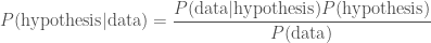
We can do this using Bayes’ theorem

\displaystyle P(\mathrm{hypothesis}|\mathrm{data}) = \frac{P(\mathrm{data}|\mathrm{hypothesis})P(\mathrm{hypothesis})}{P(\mathrm{data})}.

In this context, we give names to each of the probabilities (to make things sound extra fancy): P(\mathrm{hypothesis}|\mathrm{data}) is the posterior, because it’s what we get at the end; P(\mathrm{data}|\mathrm{hypothesis}) is the likelihood, it’s what you may remember calculating in statistics classes; P(\mathrm{hypothesis}) is the prior, because it’s what we believed about our hypothesis before we got the data, and P(\mathrm{data}) is the evidence. If ever you hear of someone doing something in a Bayesian way, it just means they are using the formula above. I think it’s rather silly to point this out, as it’s really the only logical way to do science, but people like to put “Bayesian” in the title of their papers as it sounds cool.

Whenever you get some new information, some new data, you should update your belief in your hypothesis using the above. The prior is what you believed about hypothesis before, and the posterior is what you believe after (you’ll use this posterior as your prior next time you learn something new). There are a couple of examples below, but before we get there I will take a moment to discuss priors.

About priors: what we already know

There have been many philosophical arguments about the use of priors in science. People worry that what you believe affects the results of science. Surely science should be above such things: it should be about truth, and should not be subjective! Sadly, this is not the case. Using Bayes’ theorem is the only logical thing to do. You can’t calculate a probability of what you believe after you get some data unless you know what you believed beforehand. If this makes you unhappy, just remember that when we changed our probability for it being raining outside, it didn’t change whether it was raining or not. If two different people use two different priors they can get two different results, but that’s OK, because they know different things, and so they should expect different things to happen.

To try to convince yourself that priors are necessary, consider the case that you are Sherlock Holmes (one of the modern versions), and you are trying to solve a bank robbery. There is a witness who saw the getaway, and they can remember what they saw with 99% accuracy (this gives the likelihood). If they say the getaway vehicle was a white transit van, do you believe them? What if they say it was a blue unicorn? In both cases the witness is the same, the likelihood is the same, but one is much more believable than the other. My prior that the getaway vehicle is a transit van is much greater than my prior for a blue unicorn: the latter can’t carry nearly as many bags of loot, and so is a silly choice.

If you find that changing your prior (to something else sensible) significantly changes your results, this just means that your data don’t tell you much. Imagine that you checked the weather forecast before leaving the office and it said “cloudy with 0–100% chance of precipitation”. You basically believe the same thing before and after. This really means that you need more (or better) data. I’ll talk about some good ways of calculating priors in the future.

Solving the inverse problem

Example 1: Doughnut allergy

We shall now attempt to use Bayes’ theorem to calculate some posterior probabilities. First, let’s consider a worrying situation. Imagine there is a rare genetic disease that makes you allergic to doughnuts. One in a million people have this disease, that only manifests later in life. You have tested positive. The test is 99% successful at detecting the disease if it is present, and returns a false positive (when you don’t have the disease) 1% of the time. How worried should you be? Let’s work out the probability of having the disease given that you tested positive

\displaystyle P(\mathrm{allergy}|\mathrm{positive}) = \frac{P(\mathrm{positive}|\mathrm{allergy})P(\mathrm{allergy})}{P(\mathrm{positive})}.

Our prior for having the disease is given by how common it is, P(\mathrm{allergy}) = 10^{-6}. The prior probability of not having the disease is P(\mathrm{no\: allergy}) = 1 - P(\mathrm{allergy}). The likelihood of our positive result is P(\mathrm{positive}|\mathrm{allergy}) = 0.99, which seems worrying. The evidence, the total probability of testing positive P(\mathrm{positive}) is found by adding the probability of a true positive and a false positive

 P(\mathrm{positive}) = P(\mathrm{positive}|\mathrm{allergy})P(\mathrm{allergy}) + P(\mathrm{positive}|\mathrm{no\: allergy})P(\mathrm{no\: allergy}).

The probability of a false positive is P(\mathrm{positive}|\mathrm{no\: allergy}) = 0.01. We thus have everything we need. Substituting everything in, gives

\displaystyle P(\mathrm{allergy}|\mathrm{positive}) = \frac{0.99 \times 10^{-6}}{0.99 \times 10^{-6} + 0.01 \times (1 - 10^{-6})} = 9.899 \times 10^{-5}.

Even after testing positive, you still only have about a one in ten thousand chance of having the allergy. While it is more likely that you have the allergy than a random member of the public, it’s still overwhelmingly probable that you’ll be fine continuing to eat doughnuts. Hurray!

Doughnut love

Doughnut love: probably fine.

Example 2: Boys, girls and water balloons

Second, imagine that Iris has three children. You know she has a boy and a girl, but you don’t know if she has two boys or two girls. You pop around for doughnuts one afternoon, and a girl opens the door. She is holding a large water balloon. What’s the probability that Iris has two girls? We want to calculate the posterior

\displaystyle P(\mathrm{two\: girls}|\mathrm{girl\:at\:door}) = \frac{P(\mathrm{girl\:at\:door}|\mathrm{two\: girls})P(\mathrm{two\: girls})}{P(\mathrm{girl\:at\:door})}.

As a prior, we’d expect boys and girls to be equally common, so P(\mathrm{two\: girls}) = P(\mathrm{two\: boys}) = 1/2. If we assume that it is equally likely that any one of the children opened the door, then the likelihood that one of the girls did so when their are two of them is P(\mathrm{girl\:at\:door}|\mathrm{two\: girls}) = 2/3. Similarly, if there were two boys, the probability of a girl answering the door is P(\mathrm{girl\:at\:door}|\mathrm{two\: boys}) = 1/3. The evidence, the total probability of a girl being at the door is

P(\mathrm{girl\:at\:door}) =P(\mathrm{girl\:at\:door}|\mathrm{two\: girls})P(\mathrm{two\: girls}) +P(\mathrm{girl\:at\:door}|\mathrm{two\: boys}) P(\mathrm{two\: boys}).

Using all of these,

\displaystyle P(\mathrm{two\: girls}|\mathrm{girl\:at\:door}) = \frac{(2/3)(1/2)}{(2/3)(1/2) + (1/3)(1/2)} = \frac{2}{3}.

Even though we already knew there was at least one girl, seeing a girl first makes it much more likely that the Iris has two daughters. Whether or not you end up soaked is a different question.

Example 3: Fudge!

Finally, we shall return to the case of Ted and his overconsumption of fudge. Ted claims to have eaten a lethal dose of fudge. Given that he is alive to tell the anecdote, what is the probability that he actually ate the fudge? Here, our data is that Ted is alive, and our hypothesis is that he did eat the fudge. We have

\displaystyle P(\mathrm{fudge}|\mathrm{survive}) = \frac{P(\mathrm{survive}|\mathrm{fudge})P(\mathrm{fudge})}{P(\mathrm{survive})}.

This is a case where our prior, the probability that he would eat a lethal dose of fudge P(\mathrm{fudge}), makes a difference. We know the probability of surviving the fatal dose is P(\mathrm{survive}|\mathrm{fudge}) = 0.5. The evidence, the total probability of surviving P(\mathrm{survive}),  is calculated by considering the two possible sequence of events: either Ted ate the fudge and survived or he didn’t eat the fudge and survived

P(\mathrm{survive}) = P(\mathrm{survive}|\mathrm{fudge})P(\mathrm{fudge}) + P(\mathrm{survive}|\mathrm{no\: fudge})P(\mathrm{no\: fudge}).

We’ll assume if he didn’t eat the fudge he is guaranteed to be alive, P(\mathrm{survive}| \mathrm{no\: fudge}) = 1. Since Ted either ate the fudge or he didn’t P(\mathrm{fudge}) + P(\mathrm{no\: fudge}) = 1. Therefore,

P(\mathrm{survive}) = 0.5 P(\mathrm{fudge}) + [1 - P(\mathrm{fudge})] = 1 - 0.5 P(\mathrm{fudge}).

This gives us a posterior

\displaystyle P(\mathrm{fudge}|\mathrm{survive}) = \frac{0.5 P(\mathrm{fudge})}{1 - 0.5 P(\mathrm{fudge})}.

We just need to decide on a suitable prior.

If we believe Ted could never possibly lie, then he must have eaten that fudge and P(\mathrm{fudge}) = 1. In this case,

\displaystyle P(\mathrm{fudge}|\mathrm{survive}) = \frac{0.5}{1 - 0.5} = 1.

Since we started being absolutely sure, we end up being absolutely sure: nothing could have changed our mind! This is a poor prior: it is too strong, we are being closed-minded. If you are closed-minded you can never learn anything new.

If we don’t know who Ted is, what fudge is, or the ease of consuming a lethal dose, then we might assume an equal prior on eating the fudge and not eating the fudge, P(\mathrm{fudge}) = 0.5. In this case we are in a state of ignorance. Our posterior is

\displaystyle P(\mathrm{fudge}|\mathrm{survive}) = \frac{0.5 \times 0.5}{1 - 0.5 \times 0.5} = \frac{1}{3}.

 Even though we know nothing, we conclude that it’s more probable that the Ted did not eat the fudge. In fact, it’s twice as probable that he didn’t eat the fudge than he did as P(\mathrm{no\: fudge}|\mathrm{survive}) = 1 -P(\mathrm{fudge}|\mathrm{survive}) = 2/3.

In reality, I think that it’s extremely improbable anyone could consume a lethal dose of fudge. I’m fairly certain that your body tries to protect you from such stupidity by expelling the fudge from your system before such a point. However, I will concede that it is not impossible. I want to assign a small probability to P(\mathrm{fudge}). I don’t know if this should be one in a thousand, one in a million or one in a billion, but let’s just say it is some small value p. Then

\displaystyle P(\mathrm{fudge}|\mathrm{survive}) = \frac{0.5 p}{1 - 0.5 p} \approx 0.5 p.

as the denominator is approximately one. Whatever small probability I pick, it is half as probable that Ted ate the fudge.

Mr. Impossible

I would assign a much higher probability to Mr. Impossible being able to eat that much fudge than Ted.

While it might not be too satisfying that we can’t come up with incontrovertible proof that Ted didn’t eat the fudge, we might be able to shut him up by telling him that even someone who knows nothing would think his story is unlikely, and that we will need much stronger evidence before we can overcome our prior.

Homework example: Monty Hall

You now have all the tools necessary to tackle the Monty Hall problem, one of the most famous probability puzzles:

You are on a game show and are given the choice of three doors. Behind one is a car (a Lincoln Continental), but behind the others are goats (which you don’t want). You pick a door. The host, who knows what is behind the doors, opens another door to reveal goat. They then offer you the chance to switch doors. Should you stick with your current door or not? — Monty Hall problem

You should be able to work out the probability of winning the prize by switching and sticking. You can’t guarantee you win, but you can maximise your chances.

Summary

Whenever you encounter new evidence, you should revise how probable you think things are. This is true in science, where we perform experiments to test hypotheses; it is true when trying to solve a mystery using evidence, or trying to avoid getting a goat on a game show. Bayes’ theorem is used to update probabilities. Although Bayes’ theorem itself is quite simple, calculating likelihoods, priors and evidences for use in it can be difficult. I hope to return to all these topics in the future.