One of the great discoveries that came with our first observation of gravitational waves was that black holes can merge—two black holes in a binary can come together and form a bigger black hole. This had long been predicted, but never before witnessed. If black holes can merge once, can they go on to merge again? In this paper, we calculated how to identify a binary containing a second-generation black hole formed in a merger.
Merging black holes
Black holes have two important properties: their mass and their spin. When two black holes merge, the resulting black hole has:
A mass which is almost as big as the sum of the masses of its two parents. It is a little less (about 5%) as some of the energy is radiated away as gravitational waves.
A spin which is around 0.7. This is set by the angular momentum of the two black holes as they plunge in together. For equal-mass black holes, the orbit of the two black holes will give about enough angular momentum for the final black hole to be about 0.7. The spins of the two parent black holes will cause a bit a variation around this, depending upon the orientations of their spins. For more unequal mass binaries, the spin of the larger parent black hole becomes more important.
To look for second-generation (or higher) black holes formed in mergers, we need to look for more massive black holes with spins of about 0.7 [bonus note].
Combining black holes. The result of a merger is a larger black hole with significant spin. From Dawn Finney.
The difficult bit here is that we don’t know the distribution of masses and spins of the initial first-generation black holes. What is they naturally form with spins of 0.7? How can you tell if a black hole is unexpectedly large if you don’t know what sizes to expect? With the discovery of the 10 binary black holes found in our first and second observing runs, we are able to start making inferences about the properties of black holes—using these measurements of the population, we can estimate how probable it is that a binary contains a second generation black hole versus containing two first generation black hole.
GW170729
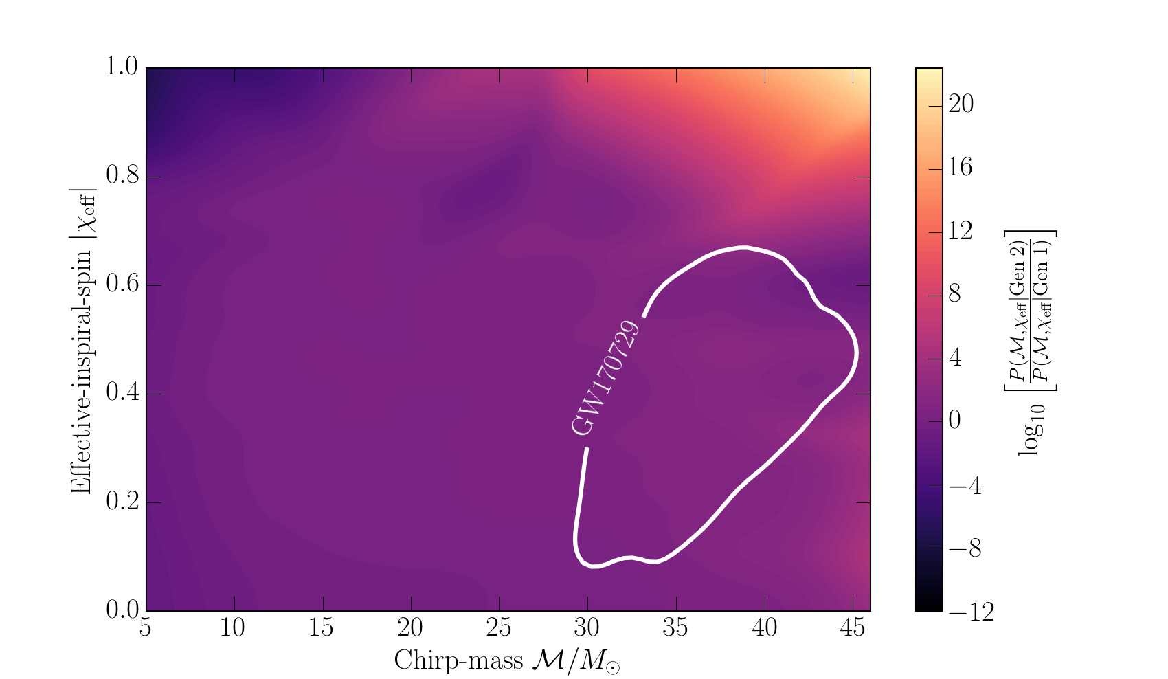
Amongst the black holes observed in O1 and O2, the source of GW170729 stands out. It is both the most massive, and one of only two systems (the other being GW151226) showing strong evidence for spin. This got me wondering if it could be a second-generation system? The high mass would be explained as we have a second-generation black hole, and the spin is larger than usual as a spin 0.7 sticks out.
Chase Kimball worked out the relative probability of getting a system with a given chirp mass and effective inspiral spin for a binary with a second-generation black hole verses a binary with only first-generation black holes. We worked in terms of chirp mass and effective inspiral spin, as these are the properties we measure well from a gravitational-wave signal.
Relative likelihood of a binary black hole being second-generation versus first-generation for different values of the chirp mass and the magnitude of the effective inspiral spin. The white contour gives the 90% credible area for GW170729. Figure 1 of Kimball et al. (2019).
The plot above shows the relative probabilities. Yellow indicate chirp mass and effective inspiral spins which are more likely with second-generation systems, while dark purple indicates values more likely with first-generation systems.. The first thing I realised was my idea about the spin was off. We expect binaries with second-generation black holes to be formed dynamically. Following the first merger, the black hole wander around until it gets close enough to form a new binary with a new black hole. For dynamically formed binaries the spins should be randomly distributed. This means that there’s only a small probability of having a spin aligned with the orbital angular momentum as measured for GW170729. Most of the time, you’d measure an effective inspiral spin of around zero.
Since we don’t know exactly the chirp mass and effective inspiral spin for GW170729, we have to average over our uncertainty. That gives the ratio of the probability of observing GW170729 given a second-generation source, verses given a first-generation source. Using different inferred black hole populations (for example, ones inferred including and excluding GW170729), we find ratios of between 0.2 (meaning the first-generation origin is more likely) and 16 (meaning second generation is more likely). The results change significantly as the result is sensitive to the maximum mass of a black hole. If we include GW170729 in our population inference for first-generation systems, the maximum mass goes up, and it’s easier to explain the system as first-generation (as you’d expect).
Before you place your bets, there is one more piece to the calculation. We have calculated the relative probabilities of the observed properties assuming either first-generation black holes or a second-generation black hole, but we have not folded in the relative rates of mergers [bonus note]. We expect first-generation only binaries to be more common than ones containing second generation black holes. In simulations of globular clusters, at most about 20% of merging binaries are with second-generation black holes. For binaries not in an environment like a globular cluster (where there are lots of nearby black holes to grab), we expect the fraction of second-generation black holes in binaries to be basically zero. Therefore, on balance we have at best a weak preference for a second-generation black hole and most probably just two first-generation black holes in GW170729’s source, despite its large mass.
Verdict
What we have learnt from this calculation is that it seems that all of the first 10 binary black holes contain only first-generation black holes. It is safe to infer the properties of first-generation black holes from these observations. Detecting second-generation black holes requires knowledge of this distribution, and crucially if there is a maximum mass. As we get more detection, we’ll be able to pin this down. There is still a lot to learn about the full black hole family.
If you’d like to understand our calculation, the paper is extremely short. It is therefore an excellent paper to bring to journal club if you are a PhD student who forgot you were presenting this week…
I was asked how we could tell if the black holes we were seeing were themselves the results of mergers back in 2016 when I was giving a talk to the Carolian Astronomical Society. It was a good question. I explained about the masses and spins, but I didn’t think about how to actually do the analysis to infer if we had a merger. I now make a note to remember any questions I’m asked, as they can be good inspiration for projects!
Bayes factor and odds ratio
The quantity we work out in the paper is the Bayes factor for a second-generation system verses a first-generation one
which gives the betting odds for the two scenarios. The convert the Bayes factor into an odds ratio we need the prior odds
.
We’re currently working on a better way to fold these pieces together.
1000 words
As this was a quick calculation, we thought it would be a good paper to be a Research Note. Research Notes are limited to 1000 words, which is a tough limit. We carefully crafted the document, using as many word-saving measures (such as abbreviations), as we could. We made it to the limit by our counting, only to submit and find that we needed to share another 100 off! Fortunately, the arXiv [bonus bonus note] is more forgiving, so you can read our more relaxed (but still delightfully short) version there. It’s the one I’d recommend.
arXiv
For those reading who are not professional physicists, the arXiv (pronounced archive, as the X is really the Greek letter chi χ) is a preprint server. It where physicists can post version of their papers ahead of publication. This allows sharing of results earlier (both good as it can take a while to get a final published paper, and because you can get feedback before finalising a paper), and, vitally, for free. Most published papers require a subscription to read. Fine if you’re at a university, not so good otherwise. The arXiv allows anyone to read the latest research. Admittedly, you have to be careful, as not everything on the arXiv will make it through peer review, and not everyone will update their papers to reflect the published version. However, I think the arXiv is a very good thing™. There are few things I can think of which have benefited modern science as much. I would 100% support those behind the arXiv receiving a Nobel Prize, as I think it has had just as a significant impact on the development of the field as the discovery of dark matter, understanding nuclear fission, or deducing the composition of the Sun.
Where do the elements come from? Hydrogen, helium and a little lithium were made in the big bang. These lighter elements are fused together inside stars, making heavier elements up to around iron. At this point you no longer get energy out by smooshing nuclei together. To build even heavier elements, you need different processes—one being to introduce lots of extra neutrons. Adding neutrons slowly leads to creation of s-process elements, while adding then rapidly leads to the creation of r-process elements. By observing the distribution of elements, we can figure out how often these different processes operate.
Periodic table showing the origins of different elements found in our Solar System. THis plot assumes that neutron star mergers are the dominant source of r-process elements. Credit: Jennifer Johnson
It has long been theorised that the site of r-process production could be neutron star mergers. Material ejected as the stars are ripped apart or ejected following the collision is naturally neutron rich. This undergoes radioactive decay leading making r-process elements. The discovery of the first binary neutron star collision confirmed this happens. If you have any gold or platinum jewellery, it’s origins can probably be traced back to a pair of neutron stars which collided billions of years ago!
The r-process may also occur in supernova explosions. It is most likely that it occurs in both supernovae and neutron star mergers—the question is which contributes more. Figuring this out would be helpful in our quest to understand how stars live and die.
In this paper, led by Michael Zevin, we investigated the r-process elements of globular clusters. Globular clusters are big balls of stars. Apart from being beautiful, globular clusters are an excellent laboratory for testing our understanding of stars,as there are so many packed into a (relatively) small space. We considered if observations of r-process enrichment could be explained by binary neutron star mergers?
Enriching globular clusters
The stars in globular clusters are all born around the same time. They should all be made from the same stuff; they should have the same composition, aside from any elements that they have made themselves. Since r-process elements are not made in stars, the stars in a globular cluster should have the same abundances of these elements. However, measurements of elements like lanthanum and europium, show star-to-star variation in some globular clusters.
This variation can happen if some stars were polluted by r-process elements made after the cluster formed. The first stars formed from unpolluted gas, while later stars formed from gas which had been enriched, possibly with stars closer to the source being more enriched than those further away. For this to work, we need (i) a process which can happen quickly [bonus science note], as the time over which stars form is short (they are almost the same age), and (ii) something that will happen in some clusters but not others—we need to hit the goldilocks zone of something not so rare that we’d almost never since enrichment, but not so common that almost all clusters would be enriched. Can binary neutron stars merge quickly enough and with the right rate to explain r-process enrichment?
Making binary neutron stars
There are two ways of making binary neutron stars: dynamically and via isolated evolution. Dynamically formed binaries are made when two stars get close enough to form a pairing, or when a star gets close to an binary existing binary resulting in one member getting ejecting and the interloper taking its place, or when two binaries get close together, resulting in all sorts of madness (Michael has previously looked at binary black holes formed through binary–binary interactions, and I love the animations, as shown below). Isolated evolution happens when you have a pair of stars that live their entire lives together. We examined both channels.
Dynamically formed binaries
With globular clusters having so many stars in such a small space, you might think that dynamical formation is a good bet for binary neutron star formation. We found that this isn’t the case. The problem is that neutron stars are relatively light. This causes two problems. First, generally the heaviest objects generally settle in the centre of a cluster where the density is highest and binaries are most likely to form. Second, in interactions, it is typically the heaviest objects that will be left in the binary. Black holes are more massive than neutron stars, so they will initially take the prime position. Through dynamical interactions, many will be eventually ejected from the cluster; however, even then, many of the remaining stars will be more massive than the neutron stars. It is hard for neutron stars to get the prime binary-forming positions [bonus note].
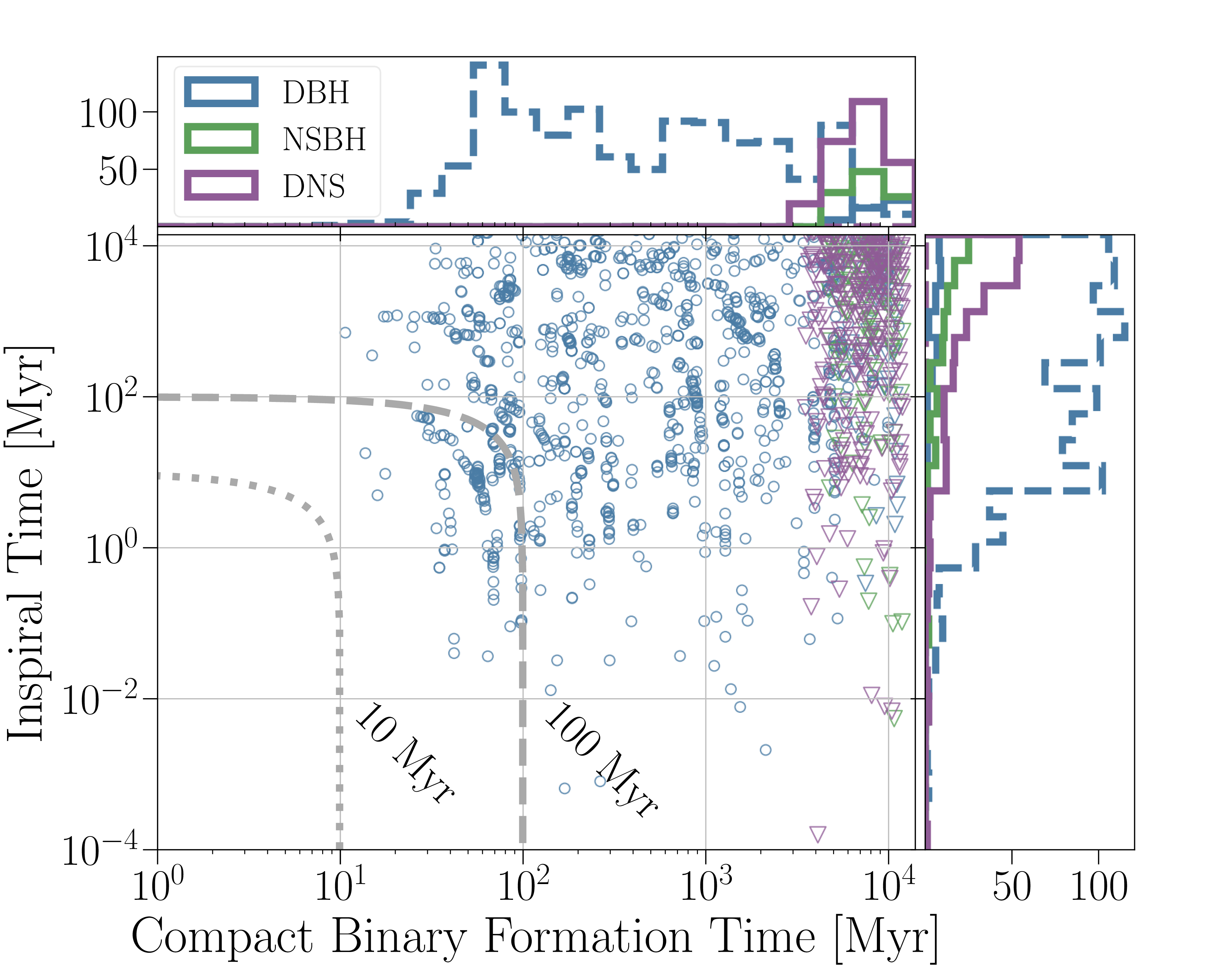
To check on the dynamical-formation potential, we performed two simulations: one with the standard mix of stars, and one ultimate best case™ where we artificially removed all the black holes. In both cases, we found that binary neutron stars take billions of years to merge. That’s far too long to lead to the necessary r-process enrichment.
Time taken for double black hole (DHB, shown in blue), neutron star–black hole (NSBH, shown in green), and double neutron star (DNS, shown in purple) [bonus note] binaries to form and then inspiral to merge in globular cluster simulations. Circles and dashed histograms show results for the standard cluster model. Triangles and solids histograms show results when black holes are artificially removed. Figure 1 of a Zevin et al. (2019).
Isolated binaries
Considering isolated binaries, we need to work out how many binary neutron stars will merge close enough to a cluster to enrich it. This requires a couple of ingredients: (I) knowing how many binary neutron stars form, and (ii) working how many are still close to the cluster when they merge. Neutron stars will get kicks when they are born in supernova explosions, and these are enough to kick them out of the cluster. So long as they merge before they get too far, that’s OK for enrichment. Therefore we need to track both those that stay in the cluster, and those which leave but merge before getting too far. To estimate the number of enriching binary neutron stars, we simulated a populations of binary stars.
The evolution of binary neutron stars can be complicated. The neutron stars form from massive stars. In order for them to end up merging, they need to be in a close binary. This means that as the stars evolve and start to expand, they will transfer mass between themselves. This mass transfer can be stable, in which case the orbit widens, faster eventually shutting off the mass transfer, or it can be unstable, when the star expands leading to even more mass transfer (what’s really important is the rate of change of the size of the star compared to the Roche lobe). When mass transfer is extremely rapid, it leads to the formation of a common envelope: the outer layers of the donor ends up encompassing both the core of the star and the companion. Drag experienced in a common envelope can lead to the orbit shrinking, exactly as you’d want for a merger, but it can be too efficient, and the two stars may merge before forming two neutron stars. It’s also not clear what would happen in this case if there isn’t a clear boundary between the envelope and core of the donor star—it’s probable you’d just get a mess and the stars merging. We used COSMIC to see the effects of different assumptions about the physics:
Model A: Our base model, which is in my opinion the least plausible. This assumes that helium stars can successfully survive a common envelope. Mass transfer from helium star will be especially important for our results, particularly what is called Case BB mass transfer [bonus note], which occurs once helium burning has finished in the core of a star, and is now burning is a shell outside the core.
Model B: Here, we assume that stars without a clear core/envelope boundary will always merge during the common envelope. Stars burning helium in a shell lack a clear core/envelope boundary, and so any common envelopes formed from Case BB mass transfer will result in the stars merging (and no binary neutron star forming). This is a pessimistic model in terms of predicting rates.
Model C: The same as Model A, but we use prescriptions from Tauris, Langer & Podsiadlowski (2015) for the orbital evolution and mass loss for mass transfer. These results show that mass transfer from helium stars typically proceeds stably. This means we don’t need to worry about common envelopes from Case BB mass transfer. This is more optimistic in terms of rates.
Model D: The same as Model C, except all stars which undergo Case BB mass transfer are assumed to become ultra-stripped. Since they have less material in their envelopes, we give them smaller supernova natal kicks, the same as electron capture supernovae.
All our models can produce some merging neutron stars within 100 million years. However, for Model B, this number is small, so that only a few percent of globular clusters would be enriched. For the others, it would be a few tens of percent, but not all. Model A gives the most enrichment. Model C and D are similar, with Model D producing slightly less enrichment.
Post-supernova binary neutron star properties (systemic velocity vs inspiral time , and orbital separation vs eccentricity ) for our population models. The lines in the left-hand plots show the bounds for a binary to enrich a cluster of a given virial radius: viable binaries are below the lines. In both plots, red, blue and green points are the binaries which could enrich clusters of virial radii 1 pc, 3 pc and 10 pc; of the other points, purple indicates systems where the secondary star went through Case BB mass transfer. Figure 2 of Zevin et al. (2019).
Maybe?
Our results show that the r-process enrichment of globular clusters could be explained by binary neutron star mergers if binaries can survive Case BB mass transfer without merging. If Case BB mass transfer is typically unstable and somehow it is possible to survive a common envelope (Model A), ~30−90% of globular clusters should be enriched (depending upon their mass and size). This rate is consistent with consistent with current observations, but it is a stretch to imagine stars surviving common envelopes in this case. However, if Case BB mass transfer is stable (Models C and D), we still have ~10−70% of globular clusters should be enriched. This could plausibly explain everything! If we can measure the enrichment in more clusters and accurately pin down the fraction which are enriched, we may learn something important about how binaries interact.
However, for our idea to work, we do need globular clusters to form stars over an extended period of time. If there’s no gas around to absorb the material ejected from binary neutron star mergers and then form new stars, we have not cracked the problem. The plot below shows that the build up of enriching material happens at around 40 million years after the initial start formation. This is when we need the gas to be around. If this is not the case, we need a different method of enrichment.
Probability of cluster enrichment and number of enriching binary neutron star mergers per cluster as a function of the timescale of star formation . Dashed lines are used of a cluster of a million solar masses and solid lines are used for a cluster of half this mass. Results are shown for Model D. The build up happens around the same time in different models. Figure 5 in Zevin et al. (2019).
It may be interesting to look again at r-process enrichment from supernova.
The most recent gravitational-wave detection, GW190425, comes from a binary neutron star system of an unusually high mass. It’s mass is much higher than the population of binary neutron stars observed in our Galaxy. One explanation for this could be that it represents a population which is short lived, and we’d be unlikely to spot one in our Galaxy, as they’re not around for long. Consequently, the same physics may be important both for this study of globular clusters and for explaining GW190425.
Gravitational-wave sources and dynamical formation
The question of how do binary neutron stars form is important for understanding gravitational-wave sources. The question of whether dynamically formed binary neutron stars could be a significant contribution to the overall rate was recently studied in detail in a paper led by Northwestern PhD student Claire Ye. The conclusions of this work was that the fraction of binary neutron stars formed dynamically in globular clusters was tiny (in agreement with our results). Only about 0.001% of binary neutron stars we observe with gravitational waves would be formed dynamically in globular clusters.
Double vs binary
In this paper we use double black hole = DBH and double neutron star = DNS instead of the usual binary black hole = BBH and binary neutron star = BNS from gravitational-wave astronomy. The terms mean the same. I will use binary instead of double here as B is worth more than D in Scrabble.
Mass transfer cases
The different types of mass transfer have names which I always forget. For regular stars we have:
Case A is from a star on the main sequence, when it is burning hydrogen in its core.
Case B is from a star which has finished burning hydrogen in its core, and is burning hydrogen in shell/burning helium in the core.
Case C is from a start which has finished core helium burning, and is burning helium in a shell. The star will now have carbon it its core, which may later start burning too.
The situation where mass transfer is avoided because the stars are well mixed, and so don’t expand, has also been referred to as CaseM. This is more commonly known as (quai)chemically homogenous evolution.
If a star undergoes Case B mass transfer, it can lose its outer hydrogen-rich layers, to leave behind a helium star. This helium star may subsequently expand and undergo a new phase of mass transfer. The mass transfer from this helium star gets named similarly:
Case BA is from the helium star while it is on the helium main sequence burning helium in its core.
Case BB is from the helium star once it has finished core helium burning, and may be burning helium in a shell.
Case BC is from the helium star once it is burning carbon.
If the outer hydrogen-rich layers are lost during Case C mass transfer, we are left with a helium star with a carbon–oxygen core. In this case, subsequent mass transfer is named as:
Case CB if helium shell burning is on-going. (I wonder if this could lead to fast radio bursts?)
Case CC once core carbon burning has started.
I guess the naming almost makes sense. Case closed!
Page count
Don’t be put off by the length of the paper—the bibliography is extremely detailed. Michael was exceedingly proud of the number of references. I think it is the most in any non-review paper of mine!
Gravity Spy is an awesome project that combines citizen science and machine learning to classify glitches in LIGO and Virgo data. Glitches are short bursts of noise in our detectors which make analysing our data more difficult. Some glitches have known causes, others are more mysterious. Classifying glitches into different types helps us better understand their properties, and in some cases track down their causes and eliminate them! In this paper, led by Scotty Coughlin, we demonstrated the effectiveness of a new tool which are citizen scientists can use to identify new glitch classes.
The Gravity Spy project
Gravitational-wave detectors are complicated machines. It takes a lot of engineering to achieve the required accuracy needed to observe gravitational waves. Most of the time, our detectors perform well. The background noise in our detectors is easy to understand and model. However, our detectors are also subject to glitches, unusual (sometimes extremely loud and complicated) noise that doesn’t fit the usual properties of noise. Glitches are short, they only appear in a small fraction of the total data, but they are common. This makes detection and analysis of gravitational-wave signals more difficult. Detection is tricky because you need to be careful to distinguish glitches from signals (and possibly glitches and signals together), and understanding the signal is complicated as we may need to model a signal and a glitch together [bonus note]. Understanding glitches is essential if gravitational-wave astronomy is to be a success.
To understand glitches, we need to be able to classify them. We can search for glitches by looking for loud pops, whooshes and splats in our data. The task is then to spot similarities between them. Once we have a set of glitches of the same type, we can examine the state of the instruments at these times. In the best cases, we can identify the cause, and then work to improve the detectors so that this no longer happens. Other times, we might be able to find the source, but we can find one of the monitors in our detectors which acts a witness to the glitch. Then we know that if something appears in that monitor, we expect a glitch of a particular form. This might mean that we throw away that bit of data, or perhaps we can use the witness data to subtract out the glitch. Since glitches are so common, classifying them is a huge amount of work. It is too much for our detector characterisation experts to do by hand.
There are two cunning options for classifying large numbers of glitches
Get a computer to do it. The difficulty is teaching a computer to identify the different classes. Machine-learning algorithms can do this, if they are properly trained. Training can require a large training set, and careful validation, so the process is still labour intensive.
Get lots of people to help. The difficulty here is getting non-experts up-to-speed on what to look for, and then checking that they are doing a good job. Crowdsourcing classifications is something citizen scientists can do, but we will need a large number of dedicated volunteers to tackle the full set of data.
The idea behind Gravity Spy is to combine the two approaches. We start with a small training set from our detector characterization experts, and train a machine-learning algorithm on them. We then ask citizen scientists (thanks Zooniverse) to classify the glitches. We start them off with glitches the machine-learning algorithm is confident in its classification; these should be easy to identify. As citizen scientists get more experienced, they level up and start tackling more difficult glitches. The citizen scientists validate the classifications of the machine-learning algorithm, and provide a larger training set (especially helpful for the rarer glitch classes) for it. We can then happily apply the machine-learning algorithm to classify the full data set [bonus note].
How Gravity Spy works: the interconnection of machine-learning classification and citizen-scientist classification. The similarity search is used to identify glitches similar to one which do not fit into current classes. Figure 2 of Coughlin et al. (2019).
I especially like the levelling-up system in Gravity Spy. I think it helps keep citizen scientists motivated, as it both prevents them from being overwhelmed when they start and helps them see their own progress. I am currently Level 4.
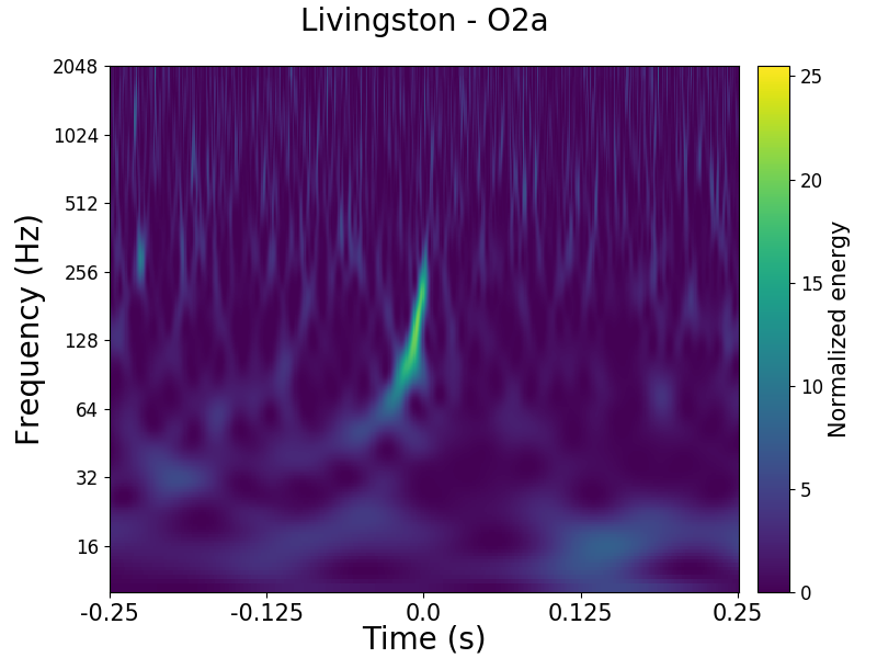
Gravity Spy works using images of the data. We show spectrograms, plots of how loud the output of the detectors are at different frequencies at different times. A gravitational wave form a binary would show a chirp structure, starting at lower frequencies and sweeping up.
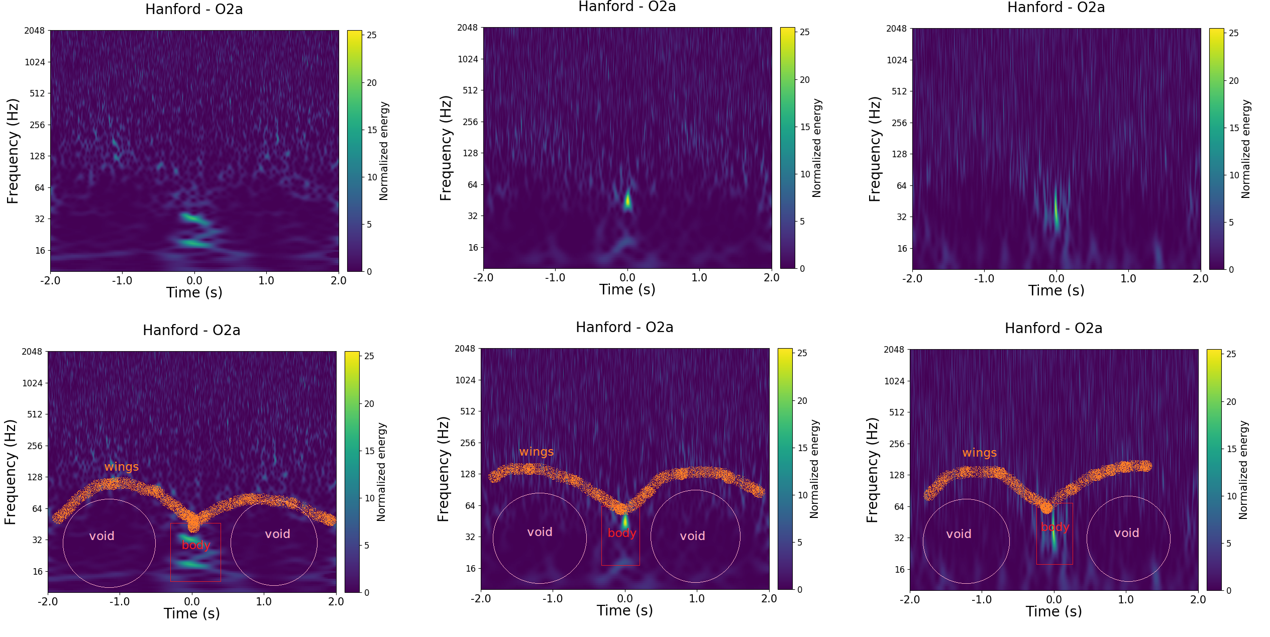
Spectrogram showing the upward-sweeping chirp of gravitational wave GW170104 as seen in Gravity Spy. I correctly classified this as a Chirp.
New glitches
The Gravity Spy system works smoothly. However, it is set up to work with a fixed set of glitch classes. We may be missing new glitch classes, either because they are rare, and hadn’t been spotted by our detector characterization team, or because we changed something in our detectors and new class arose (we expect this to happen as we tune up the detectors between observing runs). We can add more classes to our citizen scientists and machine-learning algorithm to use, but how do we spot new classes in the first place?
Our citizen scientists managed to identify a few new glitches by spotting things which didn’t fit into any of the classes. These get put in the None-of-the-Above class. Occasionally, you’ll come across similar looking glitches, and by collecting a few of these together, build a new class. The Paired Dove and Helix classes were identified early on by our citizen scientists this way; my favourite suggested new class is the Falcon [bonus note]. The difficulty is finding a large number of examples of a new class—you might only recognise a common feature after going past a few examples, backtracking to find the previous examples is hard, and you just have to keep working until you are lucky enough to be given more of the same.
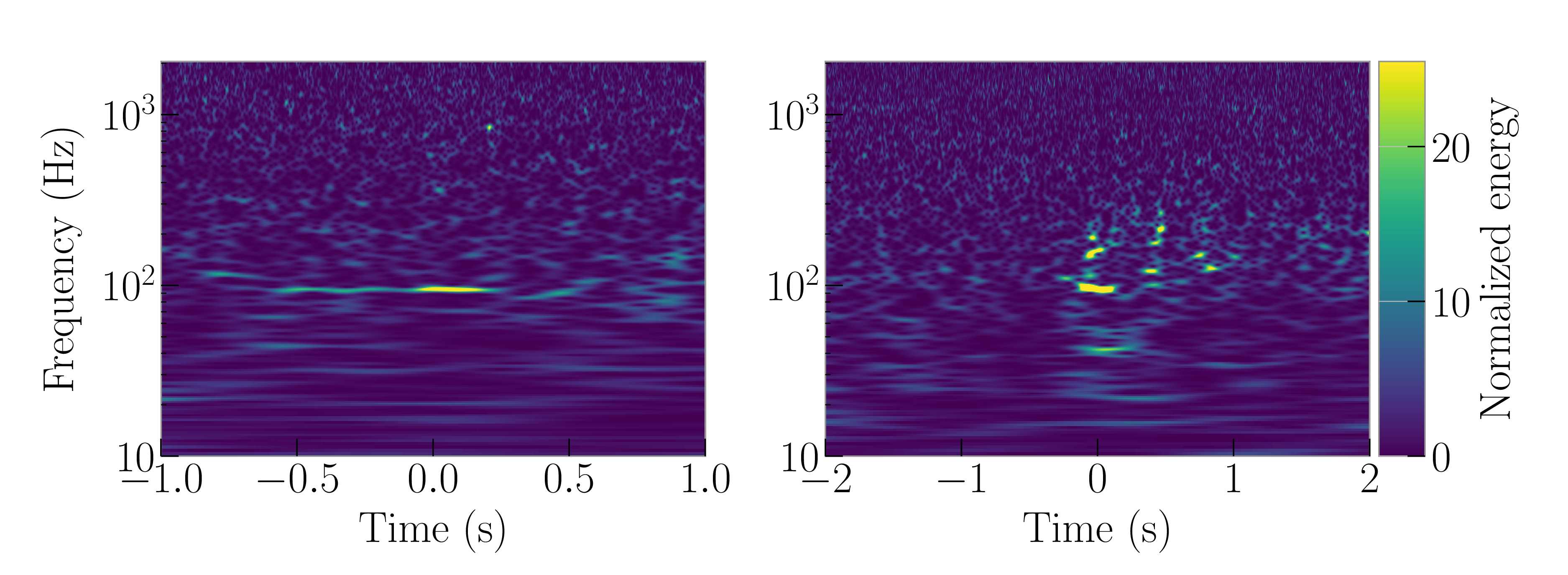
Example Helix (left) and Paired Dove glitches. These classes were identified by Gravity Spy citizen scientists. Helix glitches are related to related to hiccups in the auxiliary lasers used to calibrate the detectors by pushing on the mirrors. Paired Dove glitches are related to motion of the beamsplitter in the interferometer. Adapted from Figure 8 of Zevin et al. (2017).
To help our citizen scientists find new glitches, we created a similar search. Having found an interesting glitch, you can search for similar examples, and put quickly put together a collection of your new class. The video below shows how it works. The thing we had to work out was how to define similar?
Transfer learning
Our machine-learning algorithm only knows about the classes we tell it about. It then works out the features we distinguish the different classes, and are common to glitches of the same class. Working in this feature space, glitches form clusters of different classes.
Visualisation showing the clustering of different glitches in the Gravity Spy feature space. Each point is a different glitch from our training set. The feature space has more than three dimensions: this visualisation was made using a technique which preserves the separation and clustering of different and similar points. Figure 1 of Coughlin et al. (2019).
For our similarity search, our idea was to measure distances in feature space [bonus note for experts]. This should work well if our current set of classes have a wide enough set of features to capture to characteristics of the new class; however, it won’t be effective if the new class is completely different, so that its unique features are not recognised. As an analogy, imagine that you had an algorithm which classified M&M’s by colour. It would probably do well if you asked it to distinguish a new colour, but would probably do poorly if you asked it to distinguish peanut butter filled M&M’s as they are identified by flavour, which is not a feature it knows about. The strategy of using what a machine learning algorithm learnt about one problem to tackle a new problem is known as transfer learning, and we found this strategy worked well for our similarity search.
Raven Pecks and Water Jets
To test our similarity search, we applied it to two glitches classes not in the Gravity Spy set:
Raven Peck glitches are caused by thirsty ravens pecking ice built up along nitrogen vent lines outside of the Hanford detector. Raven Pecks look like horizontal lines in spectrograms, similar to other Gravity Spy glitch classes (like the Power Line, Low Frequency Line and 1080 Line). The similarity search should therefore do a good job, as we should be able to recognise its important features.
Water Jet glitches were caused by local seismic noise at the Hanford detector which causes loud bands which disturb the input laser optics. These glitches are found between , over which time there are 26,871 total glitches in GRavity Spy. The Water Jet glitch doesn’t have anything to do with water, it is named based on its appearance (like a fountain, not a weasel). Its features are subtle, and unlike other classes, so we would expect this to be difficult for our similarity search to handle.
These glitches appeared in the data from the second observing run. Raven Pecks appeared between 14 April and 9 August 2017, and Water Jets appeared 4 January and 28 May 2017. Over these intervals there are a total of 13,513 and 26,871 Gravity Spy glitches from all type, so even if you knew exactly when to look, you have a large number to search through to find examples.
Example Raven Peck (left) and Water Jet (right) glitches. These classes of glitch are not included in the usual Gravity Spy scheme. Adapted from Figure 3 of Coughlin et al. (2019).
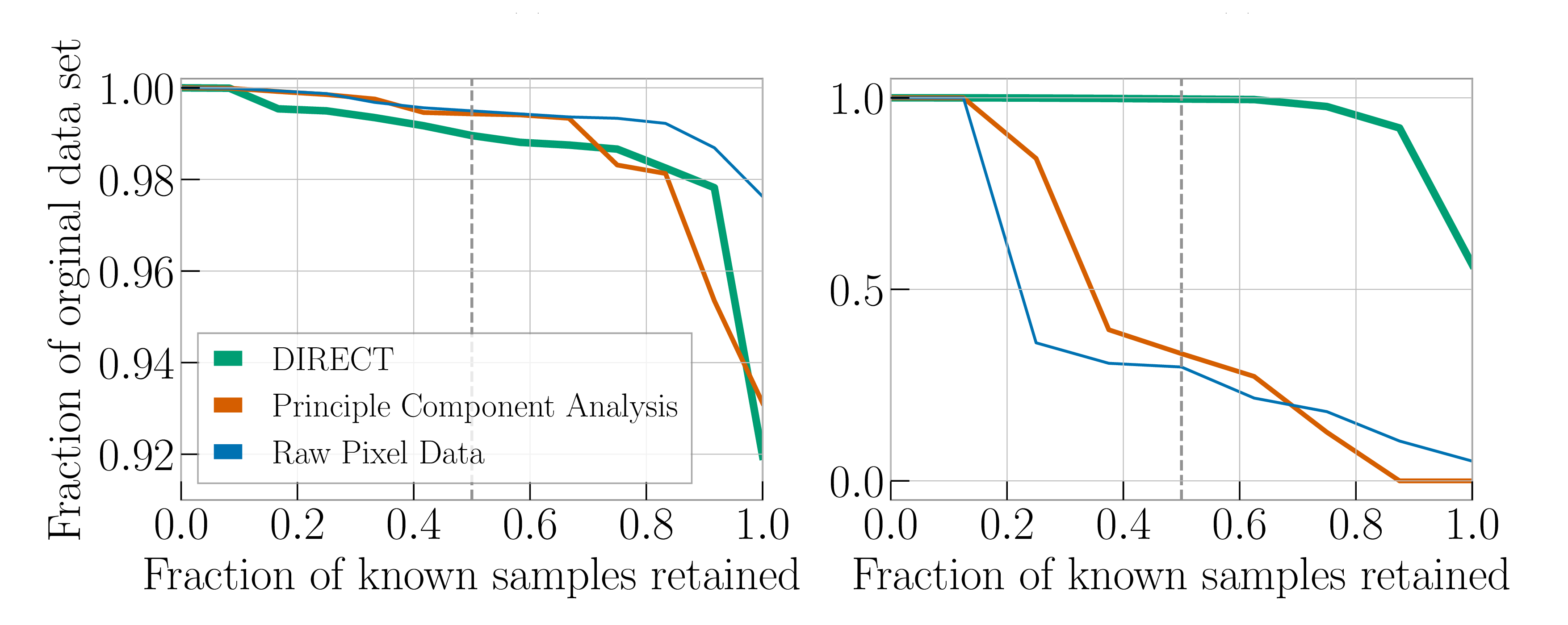
We tested using our machine-learning feature space for the similarity search against simpler approaches: using the raw difference in pixels, and using a principal component analysis to create a feature space. Results are shown in the plots below. These show the fraction of glitches we want returned by the similarity search versus the total number of glitches rejected. Ideally, we would want to reject all the glitches except the ones we want, so the search would return 100% of the wanted classes and reject almost 100% of the total set. However, the actual results will depend on the adopted threshold for the similarity search: if we’re very strict we’ll reject pretty much everything, and only get the most similar glitches of the class we want, if we are too accepting, we get everything back, regardless of class. The plots can be read as increasing the range of the similarity search (becoming less strict) as you go left to right.
Performance of the similarity search for Raven Peck (left) and Water Jet (right) glitches: the fraction of known glitches of the desired class that have a higher similarity score (compared to an example of that glitch class) than a given percentage of full data set. Results are shown for three different ways of defining similarity: the DIRECT machine-learning algorithm feature space (think line), a principal component analysis (medium line) and a comparison of pixels (thin line). Adapted from Figure 3 of Coughlin et al. (2019).
For the Raven Peck, the similarity search always performs well. We have 50% of Raven Pecks returned while rejecting 99% of the total set of glitches, and we can get the full set while rejecting 92% of the total set! The performance is pretty similar between the different ways of defining feature space. Raven Pecks are easy to spot.
Water Jets are more difficult. When we have 50% of Water Jets returned by the search, our machine-learning feature space can still reject almost all glitches. The simpler approaches do much worse, and will only reject about 30% of the full data set. To get the full set of Water Jets we would need to loosen the similarity search so that it only rejects 55% of the full set using our machine-learning feature space; for the simpler approaches we’d basically get the full set of glitches back. They do not do a good job at narrowing down the hunt for glitches. Despite our suspicion that our machine-learning approach would struggle, it still seems to do a decent job [bonus note for experts].
Do try this at home
Having developed and testing our similarity search tool, it is now live. Citizen scientists can use it to hunt down new glitch classes. Several new glitches classes have been identified in data from LIGO and Virgo’s (currently ongoing) third observing run. If you are looking for a new project, why not give it a go yourself? (Or get your students to give it a go, I’ve had some reasonable results with high-schoolers). There is the real possibility that your work could help us with the next big gravitational-wave discovery.
The best example of a gravitational-wave overlapping a glitch is GW170817. The glitch meant that the signal in the LIGO Livingston detector wasn’t immediately recognised. Fortunately, the signal in the Hanford detector was easy to spot. The glitch was analyse and categorised in Gravity Spy. It is a simple glitch, so it wasn’t too difficult to remove from the data. As our detectors become more sensitive, so that detections become more frequent, we expect that signal overlapping with glitches will become a more common occurrence. Unless we can eliminate glitches, it is only a matter of time before we get a glitch that prevents us from analysing an important signal.
Gravitational-wave alerts
In the third observing run of LIGO and Virgo, we send out automated alerts when we have a new gravitational-wave candidate. Astronomers can then pounce into action to see if they can spot anything coinciding with the source. It is important to quickly check the state of the instruments to ensure we don’t have a false alarm. To help with this, a data quality report is automatically prepared, containing many diagnostics. The classification from the Gravity Spy algorithm is one of many pieces of information included. It is the one I check first.
The Falcon
Excellent Gravity Spy moderator EcceruElme suggested a new glitch class Falcon. This suggestion was followed up by Oli Patane, they found that all the examples identified occured between 6:30 am and 8:30 am on 20 June 2017 in the Hanford detector. The instrument was misbehaving at the time. To solve this, the detector was taken out of observing mode and relocked (the equivalent of switching it off and on again). Since this glitch class was only found in this one 2-hour window, we’ve not added it as a class. I love how it was possible to identify this problematic stretch of time using only Gravity Spy images (which don’t identify when they are from). I think this could be the seed of a good detective story. The Hanfordese Falcon?
Examples of the proposed Falcon glitch class, illustrating the key features (and where the name comes from). This new glitch class was suggested by Gravity Spy citizen scientist EcceruElme.
Distance measure
We chose a cosine distance to measure similarity in feature space. We found this worked better than a Euclidean metric. Possibly because for identifying classes it is more important to have the right mix of features, rather than how significant the individual features are. However, we didn’t do a systematic investigation of the optimal means of measuring similarity.
Retraining the neural net
We tested the performance of the machine-learning feature space in the similarity search after modifying properties of our machine-learning algorithm. The algorithm we are using is a deep multiview convolution neural net. We switched the activation function in the fully connected layer of the net, trying tanh and leaukyREU. We also varied the number of training rounds and the number of pairs of similar and dissimilar images that are drawn from the training set each round. We found that there was little variation in results. We found that leakyREU performed a little better than tanh, possibly because it covers a larger dynamic range, and so can allow for cleaner separation of similar and dissimilar features. The number of training rounds and pairs makes negligible difference, possibly because the classes are sufficiently distinct that you don’t need many inputs to identify the basic features to tell them apart. Overall, our results appear robust. The machine-learning approach works well for the similarity search.
The first gravitational wave detection of LIGO and Virgo’s third observing run (O3) has been announced: GW190425! [bonus note] The signal comes from the inspiral of two objects which have a combined mass of about 3.4 times the mass of our Sun. These masses are in range expected for neutron stars, this makes GW190425 the second observation of gravitational waves from a binary neutron star inspiral (after GW170817). While the individual masses of the two components agree with the masses of neutron stars found in binaries, the overall mass of the binary (times the mass of our Sun) is noticeably larger than any previously known binary neutron star system. GW190425 may be the first evidence for multiple ways of forming binary neutron stars.
The gravitational wave signal
On 25 April 2019 the LIGO–Virgo network observed a signal. This was promptly shared with the world as candidate event S190425z [bonus note]. The initial source classification was as a binary neutron star. This caused a flurry of excitement in the astronomical community [bonus note], as the smashing together of two neutron stars should lead to the emission of light. Unfortunately, the sky localization was HUGE (the initial 90% area wass about a quarter of the sky, and the refined localization provided the next day wasn’t much improvement), and the distance was four times that of GW170817 (meaning that any counterpart would be about 16 times fainter). Covering all this area is almost impossible. No convincing counterpart has been found [bonus note].
Early sky localization for GW190425. Darker areas are more probable. This localization was circulated in GCN 24228 on 26 April and was used to guide follow-up, even though it covers a huge amount of the sky (the 90% area is about 18% of the sky).
The localization for GW19045 was so large because LIGO Hanford (LHO) was offline at the time. Only LIGO Livingston (LLO) and Virgo were online. The Livingston detector was about 2.8 times more sensitive than Virgo, so pretty much all the information came from Livingston. I’m looking forward to when we have a larger network of detectors at comparable sensitivity online (we really need three detectors observing for a good localization).
We typically search for gravitational waves by looking for coincident signals in our detectors. When looking for binaries, we have templates for what the signals look like, so we match these to the data and look for good overlaps. The overlap is quantified by the signal-to-noise ratio. Since our detectors contains all sorts of noise, you’d expect them to randomly match templates from time to time. On average, you’d expect the signal-to-noise ratio to be about 1. The higher the signal-to-noise ratio, the less likely that a random noise fluctuation could account for this.
Our search algorithms don’t just rely on the signal-to-noise ratio. The complication is that there are frequently glitches in our detectors. Glitches can be extremely loud, and so can have a significant overlap with a template, even though they don’t look anything like one. Therefore, our search algorithms also look at the overlap for different parts of the template, to check that these match the expected distribution (for example, there’s not one bit which is really loud, while the others don’t match). Each of our different search algorithms has their own way of doing this, but they are largely based around the ideas from Allen (2005), which is pleasantly readable if you like these sort of things. It’s important to collect lots of data so that we know the expected distribution of signal-to-noise ratio and signal-consistency statistics (sometimes things change in our detectors and new types of noise pop up, which can confuse things).
It is extremely important to check the state of the detectors at the time of an event candidate. In O3, we have unfortunately had to retract various candidate events after we’ve identified that our detectors were in a disturbed state. The signal consistency checks take care of most of the instances, but they are not perfect. Fortunately, it is usually easy to identify that there is a glitch—the difficult question is whether there is a glitch on top of a signal (as was the case for GW170817). Our checks revealed nothing up with the detectors which could explain the signal (there was a small glitch in Livingston about 60 seconds before the merger time, but this doesn’t overlap with the signal).
Now, the search that identified GW190425 was actually just looking for single-detector events: outliers in the distribution of signal-to-noise ratio and signal-consistency as expected for signals. This was a Good Thing™. While the signal-to-noise ratio in Livingston was 12.9 (pretty darn good), the signal-to-noise ration in Virgo was only 2.5 (pretty meh) [bonus note]. This is below the threshold (signal-to-noise ratio of 4) the search algorithms use to look for coincidences (a threshold is there to cut computational expense: the lower the threshold, the more triggers need to be checked) [bonus note]. The Bad Thing™ about GW190425 being found by the single-detector search, and being missed by the usual multiple detector search, is that it is much harder to estimate the false-alarm rate—it’s much harder to rule out the possibility of some unusual noise when you don’t have another detector to cross-reference against. We don’t have a final estimate for the significance yet. The initial estimate was 1 in 69,000 years (which relies on significant extrapolation). What we can be certain of is that this event is a noticeable outlier: across the whole of O1, O2 and the first 50 days of O3, it comes second only to GW170817. In short, we can say that GW190425 is worth betting on, but I’m not sure (yet) how heavily you want to bet.
Detection statistics for GW190425 showing how it stands out from the background. The left plot shows the signal-to-noise ratio (SNR) and signal-consistency statistic from the GstLAL algorithm, which made the detection. The coloured density plot shows the distribution of background triggers. Right shows the detection statistic from PyCBC, which combines the SNR and their signal-consistency statistic. The lines show the background distributions. GW190425 is more significant than everything apart from GW170817. Adapted from Figures 1 and 6 of the GW190425 Discovery Paper.
I’m always cautious of single-detector candidates. If you find a high-mass binary black hole (which would be an extremely short template), or something with extremely high spins (indicating that the templates don’t match unless you push to the bounds of what is physical), I would be suspicious. Here, we do have consistent Virgo data, which is good for backing up what is observed in Livingston. It may be a single-detector detection, but it is a multiple-detector observation. To further reassure ourselves about GW190425, we ran our full set of detection algorithms on the Livingston data to check that they all find similar signals, with reasonable signal-consistency test values. Indeed, they do! The best explanation for the data seems to be a gravitational wave.
The source
Given that we have a gravitational wave, where did it come from? The best-measured property of a binary inspiral is its chirp mass—a particular combination of the two component masses. For GW190425, this is solar masses (quoting the 90% range for parameters). This is larger than GW170817’s solar masses: we have a heavier binary.
Estimated masses for the two components in the binary. We show results for two different spin limits. The two-dimensional shows the 90% probability contour, which follows a line of constant chirp mass. The one-dimensional plot shows individual masses; the dotted lines mark 90% bounds away from equal mass. The masses are in the range expected for neutron stars. Figure 3 of the GW190425 Discovery Paper.
Figuring out the component masses is trickier. There is a degeneracy between the spins and the mass ratio—by increasing the spins of the components it is possible to get more extreme mass ratios to fit the signal. As we did for GW170817, we quote results with two ranges of spins. The low-spin results use a maximum spin of 0.05, which matches the range of spins we see for binary neutron stars in our Galaxy, while the high-spin results use a limit of 0.89, which safely encompasses the upper limit for neutron stars (if they spin faster than about 0.7 they’ll tear themselves apart). We find that the heavier component of the binary has a mass of – solar masses with the low-spin assumption, and – solar masses with the high-spin assumption; the lighter component has a mass – solar masses with the low-spin assumption, and – solar masses with the high-spin. These are the range of masses expected for neutron stars.
Without an electromagnetic counterpart, we cannot be certain that we have two neutron stars. We could tell from the gravitational wave by measuring the imprint in the signal left by the tidal distortion of the neutron star. Black holes have a tidal deformability of 0, so measuring a nonzero tidal deformability would be the smoking gun that we have a neutron star. Unfortunately, the signal isn’t loud enough to find any evidence of these effects. This isn’t surprising—we couldn’t say anything for GW170817, without assuming its source was a binary neutron star, and GW170817 was louder and had a lower mass source (where tidal effects are easier to measure). We did check—it’s probably not the case that the components were made of marshmallow, but there’s not much more we can say (although we can still make pretty simulations). It would be really odd to have black holes this small, but we can’t rule out than at least one of the components was a black hole.
Two binary neutron stars is the most likely explanation for GW190425. How does it compare to other binary neutron stars? Looking at the 17 known binary neutron stars in our Galaxy, we see that GW190425’s source is much heavier. This is intriguing—could there be a different, previously unknown formation mechanism for this binary? Perhaps the survey of Galactic binary neutron stars (thanks to radio observations) is incomplete? Maybe the more massive binaries form in close binaries, which are had to spot in the radio (as the neutron star moves so quickly, the radio signals gets smeared out), or maybe such heavy binaries only form from stars with low metallicity (few elements heavier than hydrogen and helium) from earlier in the Universe’s history, so that they are no longer emitting in the radio today? I think it’s too early to tell—but it’s still fun to speculate. I expect there’ll be a flurry of explanations out soon.
Comparison of the total binary mass of the 10 known binary neutron stars in our Galaxy that will merge within a Hubble time and GW190425’s source (with both the high-spin and low-spin assumptions). We also show a Gaussian fit to the Galactic binaries. GW190425’s source is higher mass than previously known binary neutron stars. Figure 5 of the GW190425 Discovery Paper.
Since the source seems to be an outlier in terms of mass compared to the Galactic population, I’m a little cautious about using the low-spin results—if this sample doesn’t reflect the full range of masses, perhaps it doesn’t reflect the full range of spins too? I think it’s good to keep an open mind. The fastest spinning neutron star we know of has a spin of around 0.4, maybe binary neutron star components can spin this fast in binaries too?
One thing we can measure is the distance to the source: . That means the signal was travelling across the Universe for about half a billion years. This is as many times bigger than diameter of Earth’s orbit about the Sun, as the diameter of the orbit is than the height of a LEGO brick. Space is big.
We have now observed two gravitational wave signals from binary neutron stars. What does the new observation mean for the merger rate of binary neutron stars? To go from an observed number of signals to how many binaries are out there in the Universe we need to know how sensitive our detectors are to the sources. This depends on the masses of the sources, since more massive binaries produce louder signals. We’re not sure of the mass distribution for binary neutron stars yet. If we assume a uniform mass distribution for neutron stars between 0.8 and 2.3 solar masses, then at the end of O2 we estimated a merger rate of –. Now, adding in the first 50 days of O3, we estimate the rate to be –, so roughly the same (which is nice) [bonus note].
Since GW190425’s source looks rather different from other neutron stars, you might be interested in breaking up the merger rates to look at different classes. Using measured masses, we can construct rates for GW170817-like (matching the usual binary neutron star population) and GW190425-like binaries (we did something similar for binary black holes after our first detection). The GW170817-like rate is –, and the GW190425-like rate is lower at –. Combining the two (Assuming that binary neutron stars are all one class or the other), gives an overall rate of –, which is not too different than assuming the uniform distribution of masses.
Given these rates, we might expect some more nice binary neutron star signals in the O3 data. There is a lot of science to come.
Future mysteries
GW190425 hints that there might be a greater variety of binary neutron stars out there than previously thought. As we collect more detections, we can start to reconstruct the mass distribution. Using this, together with the merger rate, we can start to pin down the details of how these binaries form.
As we find more signals, we should also find a few which are loud enough to measure tidal effects. With these, we can start to figure out the properties of the Stuff™ which makes up neutron stars, and potentially figure out if there are small black holes in this mass range. Discovering smaller black holes would be extremely exciting—these wouldn’t be formed from collapsing stars, but potentially could be remnants left over from the early Universe.
Probability distributions for neutron star masses and radii (blue for the more massive neutron star, orange for the lighter), assuming that GW190425’s source is a binary neutron star. The left plots use the high-spin assumption, the right plots use the low-spin assumptions. The top plots use equation-of-state insensitive relations, and the bottom use parametrised equation-of-state models incorporating the requirement that neutron stars can be 1.97 solar masses. Similar analyses were done in the GW170817 Equation-of-state Paper. In the one-dimensional plots, the dashed lines indicate the priors. Figure 16 of the GW190425 Discovery Paper.
With more detections (especially when we have more detectors online), we should also be lucky enough to have a few which are well localised. These are the events when we are most likely to find an electromagnetic counterpart. As our gravitational-wave detectors become more sensitive, we can detect sources further out. These are much harder to find counterparts for, so we mustn’t expect every detection to have a counterpart. However, for nearby sources, we will be able to localise them better, and so increase our odds of finding a counterpart. From such multimessenger observations we can learn a lot. I’m especially interested to see how typical GW170817 really was.
O3 might see gravitational wave detection becoming routine, but that doesn’t mean gravitational wave astronomy is any less exciting!
The plan for publishing papers in O3 is that we would write a paper for any particularly exciting detections (such as a binary neutron star), and then put out a catalogue of all our results later. The initial discovery papers wouldn’t be the full picture, just the key details so that the entire community could get working on them. Our initial timeline was to get the individual papers out in four months—that’s not going so well, it turns out that the most interesting events have lots of interesting properties, which take some time to understand. Who’d have guessed?
We’re still working on getting papers out as soon as possible. We’ll be including full analyses, including results which we can’t do on these shorter timescales in our catalogue papers. The catalogue paper for the first half of O3 (O3a) is currently pencilled in for April 2020.
Naming conventions
The name of a gravitational wave signal is set by the date it is observed. GW190425 is hence the gravitational wave (GW) observed on 2019 April 25th. Our candidates alerts don’t start out with the GW prefix, as we still need to do lots of work to check if they are real. Their names start with S for superevent (not for hope) [bonus bonus note], then the date, and then a letter indicating the order it was uploaded to our database of candidates (we upload candidates with false alarm rates of around one per hour, so there are multiple database entries per day, and most are false alarms). S190425z was the 26th superevent uploaded on 2019 April 25th.
What is a superevent? We call anything flagged by our detection pipelines an event. We have multiple detection pipelines, and often multiple pipelines produce events for the same stretch of data (you’d expect this to happen for real signals). It was rather confusing having multiple events for the same signal (especially when trying to quickly check a candidate to issue an alert), so in O3 we group together events from similar times into SUPERevents.
GRB 190425?
Pozanenko et al. (2019) suggest a gamma-ray burst observed by INTEGRAL (first reported in GCN 24170). The INTEGRAL team themselves don’t find anything in their data, and seem sceptical of the significance of the detection claim. The significance of the claim seems to be based on there being two peaks in the data (one about 0.5 seconds after the merger, one 5.9 seconds after the merger), but I’m not convinced why this should be the case. Nothing was observed by Fermi, which is possibly because the source was obscured by the Earth for them. I’m interested in seeing more study of this possible gamma-ray burst.
EMMA 2019
At the time of GW190425, I was attending the first day of the Enabling Multi-Messenger Astrophysics in the Big Data Era Workshop. This was a meeting bringing together many involved in the search for counterparts to gravitational wave events. The alert for S190425z cause some excitement. I don’t think there was much sleep that week.
The cafeteria at @stsci is just a war room now, with people scheduling satellites and telescopes all over the world, on the phone with colleagues, running around sharing rumors and the latest info. Exciting! @LIGO#Emma2019pic.twitter.com/2BnvOtYNcJ
The signal-to-noise ratio reported from our search algorithm for LIGO Livingston is 12.9, and the same code gives 2.5 for Virgo. Virgo was about 2.8 times less sensitive that Livingston at the time, so you might be wondering why we have a signal-to-noise ratio of 2.8, instead of 4.6? The reason is that our detectors are not equally sensitive in all directions. They are most sensitive directly to sources directly above and below, and less sensitive to sources from the sides. The relative signal-to-noise ratios, together with the time or arrival at the different detectors, helps us to figure out the directions the signal comes from.
Detection thresholds
In O2, GW170818 was only detected by GstLAL because its signal-to-noise ratios in Hanford and Virgo (4.1 and 4.2 respectively) were below the threshold used by PyCBC for their analysis (in O2 it was 5.5). Subsequently, PyCBC has been rerun on the O2 data to produce the second Open Gravitational-wave Catalog (2-OGC). This is an analysis performed by PyCBC experts both inside and outside the LIGO Scientific & Virgo Collaboration. For this, a threshold of 4 was used, and consequently they found GW170818, which is nice.
I expect that if the threshold for our usual multiple-detector detection pipelines were lowered to ~2, they would find GW190425. Doing so would make the analysis much trickier, so I’m not sure if anyone will ever attempt this. Let’s see. Perhaps the 3-OGC team will be feeling ambitious?
Rates calculations
In comparing rates calculated for this papers and those from our end-of-O2 paper, my student Chase Kimball (who calculated the new numbers) would like me to remember that it’s not exactly an apples-to-apples comparison. The older numbers evaluated our sensitivity to gravitational waves by doing a large number of injections: we simulated signals in our data and saw what fraction of search algorithms could pick out. The newer numbers used an approximation (using a simple signal-to-noise ratio threshold) to estimate our sensitivity. Performing injections is computationally expensive, so we’re saving that for our end-of-run papers. Given that we currently have only two detections, the uncertainty on the rates is large, and so we don’t need to worry too much about the details of calculating the sensitivity. We did calibrate our approximation to past injection results, so I think it’s really an apples-to-pears-carved-into-the-shape-of-apples comparison.
Paper release
The original plan for GW190425 was to have the paper published before the announcement, as we did with our early detections. The timeline neatly aligned with the AAS meeting, so that seemed like an good place to make the announcement. We managed to get the the paper submitted, and referee reports back, but we didn’t quite get everything done in time for the AAS announcement, so Plan B was to have the paper appear on the arXiv just after the announcement. Unfortunately, there was a problem uploading files to the arXiv (too large), and by the time that was fixed the posting deadline had passed. Therefore, we went with Plan C or sharing the paper on the LIGO DCC. Next time you’re struggling to upload something online, remember that it happens to Nobel-Prize winning scientific collaborations too.
On the question of when it is best to share a paper, I’m still not decided. I like the idea of being peer-reviewed before making a big splash in the media. I think it is important to show that science works by having lots of people study a topic, before coming to a consensus. Evidence needs to be evaluated by independent experts. On the other hand, engaging the entire community can lead to greater insights than a couple of journal reviewers, and posting to arXiv gives opportunity to make adjustments before you having the finished article.
I think I am leaning towards early posting in general—the amount of internal review that our Collaboration papers receive, satisfies my requirements that scientists are seen to be careful, and I like getting a wider range of comments—I think this leads to having the best paper in the end.
S
The joke that S stands for super, not hope is recycled from an article I wrote for the LIGO Magazine. The editor, Hannah Middleton wasn’t sure that many people would get the reference, but graciously printed it anyway. Did people get it, or do I need to fly around the world really fast?
Gravitational waves and gravitational lensing are two predictions of general relativity. Gravitational waves are produced whenever masses accelerate. Gravitational lensing is produced by anything with mass. Gravitational lensing can magnify images, making it easier to spot far away things. In theory, gravitational waves can be lensed too. In this paper, we looked for evidence that GW170814 might have been lensed. (We didn’t find any, but this was my first foray into traditional astronomy).
The lensing of gravitational waves
Strong gravitational lensing magnifies a signal. A gravitational wave which has been lensed would therefore have a larger amplitude than if it had not been lensed. We infer the distance to the source of a gravitational wave from the amplitude. If we didn’t know a signal was lensed, we’d therefore think the source is much closer than it really is.
The shape of the gravitational wave encodes the properties of the source. This information is what lets us infer parameters. The example signal is GW150914 (which is fairly similar to GW170814). I made this explainer with Ban Farr and Nutsinee Kijbunchoo for the LIGO Magazine.
Mismeasuring the distance to a gravitational wave has important consequences for understanding their sources. As the gravitational wave travels across the expanding Universe, it gets stretched (redshifted) so by the time it arrives at our detectors it has a longer wavelength (and shorter frequency). If we assume that a signal came from a closer source, we’ll underestimate the amount of stretching the signal has undergone, and won’t fully correct for it. This means we’ll overestimate the masses when we infer them from the signal.
This possibility got a few people thinking when we announced our first detection, as GW150914 was heavier than previously observed black holes. Could we be seeing lensed gravitational waves?
Such strongly lensed gravitational waves should be multiply imaged. We should be able to see multiple copies of the same signal which have taken different paths from the source and then are bent by the gravity of the lens to reach us at different times. The delay time between images depends on the mass of the lens, with bigger lensing having longer delays. For galaxy clusters, it can be years.
The idea
Some of my former Birmingham colleagues who study gravitational lensing, were thinking about the possibility of having multiply imaged gravitational waves. I pointed out how difficult these would be to identify. They would come from the same part of the sky, and would have the same source parameters. However, since our uncertainties are so large for gravitational wave observations, I thought it would be tough to convince yourself that you’d seen the same signal twice [bonus note]. Lensing is expected to be rare [bonus note], so would you put your money on two signals (possibly years apart) being the same, or there just happening to be two similar systems somewhere in this huge patch of the sky?
However, if there were an optical counterpart to the merger, it would be much easier to tell that it was lensed. Since we know the location of galaxy clusters which could strongly lens a signal, we can target searches looking for counterparts at these clusters. The odds of finding anything are slim, but since this doesn’t take too much telescope time to look it’s still a gamble worth taking, as the potential pay-off would be huge.
Somehow [bonus note], I got involved in observing proposals to look for strongly lensed. We got everything in place for the last month of O2. It was just one month, so I wasn’t anticipating there being that much to do. I was very wrong.
GW170814
For GW170814 there were a couple of galaxy clusters which could serve as being strong gravitational lenses. Abell 3084 started off as the more probably, but as the sky localization for GW170814 was refined, SMACS J0304.3−4401 looked like the better bet.
Sky localization for GW170814 and the galaxy clusters Abell 3084 (filled circle), and SMACS J0304.3−4401 (open). The left plot shows the low-latency Bayestar localization (LIGO only dotted, LIGO and Virgo solid), and the right shows the refined LALInference sky maps (solid from GCN 21493, which we used for our observations, and dotted from GWTC-1). The dashed lines shows the Galactic plane. Figure 1 of Smith et al. (2019).
That’s right, absolutely nothing! [bonus note] That’s not actually too surprising. GW170814‘s source was identified as a binary black hole—assuming no lensing, its source binary had masses around 25 and 30 solar masses. We don’t expect significant electromagnetic emission from a binary black hole merger (which would make it a big discovery if found, but that is a long shot). If there source were lensed, we would have overestimated the source masses, but to get the source into the neutron star mass range would take a ridiculous amount of lensing. However, the important point is that we have demonstrated that such a search for strong lensed images is possible!
The future
In O3 [bonus notebonus note], the team has been targeting lower mass systems, where a neutron star may get mislabelled as a black hole by mistake due to a moderate amount of lensing. A false identification here could confuse our understanding of the minimum mass of a black hole, and also mean that we miss all sorts of lovely multimessenger observations, so this seems like a good plan to me.
It is possible to do a statistical analysis to calculate the probability of two signals being lensed images of each. The best attempt I’ve seen at this is Hannuksela et al. (2019). They do a nice study considering lensing by galaxies (and find nothing conclusive).
Biasing merger rates
If we included lensed events in our calculations of the merger rate density (the rate of mergers per unit volume of space), without correcting for them being lensed, we would overestimate the merger rate density. We’d assume that all our mergers came from a smaller volume of space than they actually did, as we wouldn’t know that the lensed events are being seen from further away. As long as the fraction of lensed events is small, this shouldn’t be a big problem, so we’re probably safe not to worry about it.
Slippery slope
What actually happened was my then boss, Alberto Vecchio, asked me to do some calculations based upon the sky maps for our detections in O1 as they’d only take me 5 minutes. Obviously, there were then more calculations, advice about gravitational wave alerts, feedback on observing proposals… and eventually I thought that if I’d put in this much time I might as well get a paper to show for it.
It was interesting to see how electromagnetic observing works, but I’m not sure I’d do it again.
Upper limits
Following tradition, when we don’t make a detection, we can set an upper limit on what could be there. In this case, we conclude that there is nothing to see down to an i-band magnitude of 25. This is pretty faint, about 40 million times fainter than something you could see with the naked eye (translating to visibly light). We can set such a good upper limit (compared to other follow-up efforts) as we only needed to point the telescopes at a small patch of sky around the galaxy clusters, and so we could leave them staring for a relatively long time.
O3 lensing hype
In O3, two gravitational wave candidates (S190828j and S190828l) were found just 21 minutes apart—this, for reasons I don’t entirely understand, led to much speculation that they were multiple images of a gravitationally lensed source. For a comprehensive debunking, follow this Twitter thread.


 vs inspiral time
  , and orbital separation
  vs eccentricity
  ) for our population models. The lines in the left-hand plots show the bounds for a binary to enrich a cluster of a given
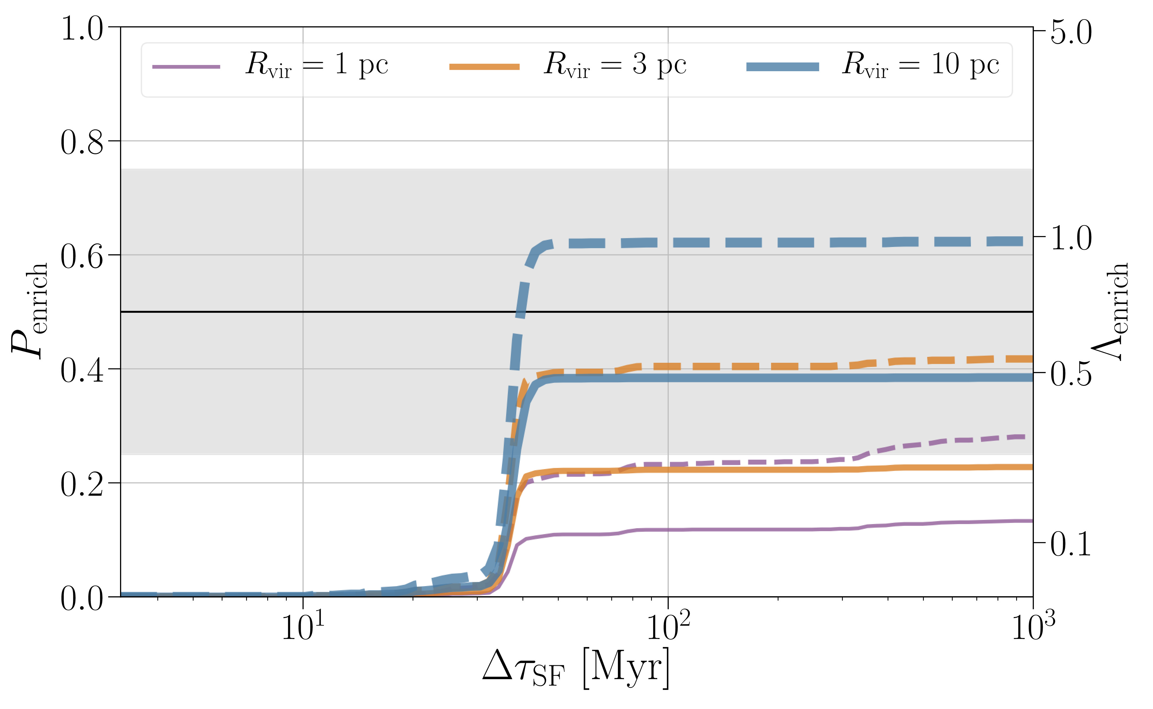
 and number of enriching binary neutron star mergers per cluster
  as a function of the timescale of star formation
  . Dashed lines are used of a cluster of a million solar masses and solid lines are used for a cluster of half this mass. Results are shown for Model D. The build up happens around the same time in different models. Figure 5 in


 solar masses (quoting the 90% range for parameters). This is larger than GW170817’s
  solar masses: we have a heavier binary.
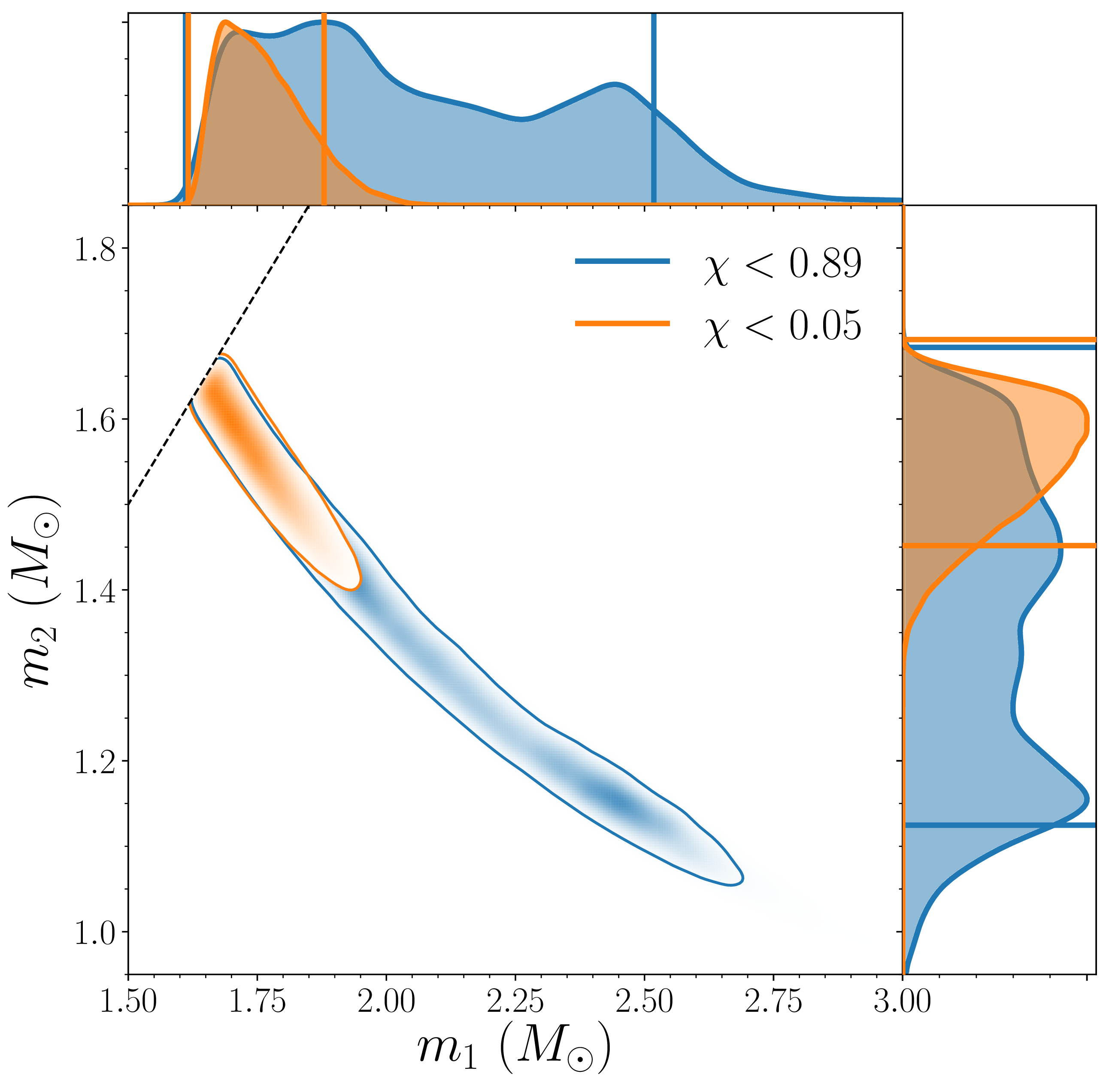
 –
– solar masses with the low-spin assumption, and
  –
– solar masses with the high-spin assumption; the lighter component has a mass
  –
– solar masses with the low-spin assumption, and
  –
– solar masses with the high-spin. These are the range of masses expected for neutron stars.
 . That means the signal was travelling across the Universe for about half a billion years. This is as many times bigger than diameter of Earth’s orbit about the Sun, as the diameter of the orbit is than the height of a LEGO brick. Space is big.
 –
– . Now, adding in the first 50 days of O3, we estimate the rate to be
  –
– , so roughly the same (which is nice) [
 , and the GW190425-like rate is lower at
  –
– . Combining the two (Assuming that binary neutron stars are all one class or the other), gives an overall rate of
  –
– , which is not too different than assuming the uniform distribution of masses.


