There has been some recent excitement about the claimed identification of a 400-solar-mass black hole. A team of scientists have recently published a letter in the journal Nature where they show how X-ray measurements of a source in the nearby galaxy M82 can be interpreted as originating from a black hole with mass of around 400 times the mass of the Sun—from now on I’ll use 


Mass of black holes
In principle, a black hole can have any mass. To form a black hole you just need to squeeze mass down into a small enough space. For the something the mass of the Earth, you need to squeeze down to a radius of about 9 mm and for something about the mass of the Sun, you need to squeeze to a radius of about 3 km. Black holes are pretty small! Most of the time, things don’t collapse to form black holes because they materials they are made of are more than strong enough to counterbalance their own gravity.

These innocent-looking marshmallows could collapse down to form black holes if they were squeezed down to a size of about 10−29 m. The only thing stopping this is the incredible strength of marshmallow when compared to gravity.
Stellar-mass black holes
Only very massive things, where gravitational forces are immense, collapse down to black holes. This happens when the most massive stars reach the end of their lifetimes. Stars are kept puffy because they are hot. They are made of plasma where all their constituent particles are happily whizzing around and bouncing into each other. This can continue to happen while the star is undergoing nuclear fusion which provides the energy to keep things hot. At some point this fuel runs out, and then the core of the star collapses. What happens next depends on the mass of the core. The least massive stars (like our own Sun) will collapse down to become white dwarfs. In white dwarfs, the force of gravity is balanced by electrons. Electrons are rather anti-social and dislike sharing the same space with each other (a concept known as the Pauli exclusion principle, which is a consequence of their exchange symmetry), hence they put up a bit of a fight when squeezed together. The electrons can balance the gravitational force for masses up to about 


Collapsing stars produce the imaginatively named stellar-mass black holes, as they are about the same mass as stars. Stars lose a lot of mass during their lifetime, so the mass of a newly born black hole is less than the original mass of the star that formed it. The maximum mass of stellar-mass black holes is determined by the maximum size of stars. We have good evidence for stellar-mass black holes, for example from looking at X-ray binaries, where we see a hot disc of material swirling around the black hole.
Massive black holes
We also have evidence for another class of black holes: massive black holes, MBHs to their friends, or, if trying to sound extra cool, supermassive black holes. These may be 

We think that there is an MBH at the centre of pretty much every galaxy, like there’s a hazelnut at the centre of a Ferrero Rocher (in this analogy, I guess the Nutella could be delicious dark matter). From the masses we’ve measured, the properties of these black holes is correlated with the properties of their surrounding galaxies: bigger galaxies have bigger MBHs. The most famous of these correlations is the M–sigma relation, between the mass of the black hole (

MBHs can grow by accreting matter (swallowing up clouds of gas or stars that stray too close) or by merging with other MBHs (we know galaxies merge). The rather embarrassing problem, however, is that we don’t know what the MBHs have grown from. There are really huge MBHs already present in the early Universe (they power quasars), so MBHs must be able to grow quickly. Did they grow from regular stellar-mass black holes or some form of super black hole that formed from a giant star that doesn’t exist today? Did lots of stellar-mass black holes collide to form a seed or did material just accrete quickly? Did the initial black holes come from somewhere else other than stars, perhaps they are leftovers from the Big Bang? We don’t have the data to tell where MBHs came from yet (gravitational waves could be useful for this).
Intermediate-mass black holes
However MBHs grew, it is generally agreed that we should be able to find some intermediate-mass black holes: black holes which haven’t grown enough to become IMBHs. These might be found in dwarf galaxies, or maybe in globular clusters (giant collections of stars that formed together), perhaps even in the centre of galaxies orbiting an MBH. Finding some IMBHs will hopefully tell us about how MBHs formed (and so, possibly about how galaxies formed too).
IMBHs have proved elusive. They are difficult to spot compared to their bigger brothers and sisters. Not finding any might mean we’d need to rethink our ideas of how MBHs formed, and try to find a way for them to either be born about a million times the mass of the Sun, or be guaranteed to grow that big. The finding of the first IMBH tells us that things are more like common sense would dictate: black holes can come in the expected range of masses (phew!). We now need to identify some more to learn about their properties as a population.
In conclusion, black holes can come in a range of masses. We know about the smaller stellar-mass ones and the bigger massive black holes. We suspect that the bigger ones grow from smaller ones, and we now have some evidence for the existence of the hypothesised intermediate-mass black holes. Whatever their size though, black holes are awesome, and they shouldn’t worry about their weight.
 ,
,  , etc., or as
  where the subscript
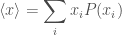
  is used as shorthand to indicate any of the possible outcomes. The probability of the numeric value being a particular
  . For rolling our dice, the outcomes are one to six (
 ,
,  , etc.) and the probabilities are
 .
. ,
, means
means  .
.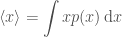 ,
, is the probability density function.
 and find out how high it needs to be to be worthwhile. We can use the expectation value to calculate how much we should expect to pay, if this is less than the bill as it stands, it’s worth giving it a go, if the expectation value is larger than the original bill, we should expect to pay more (and so probably shouldn’t play). The expectation value is
 ,
, is less than one, so if
  , it’s worth playing. If we were tossing a (fair) coin, we’d expect to come out even, if we had to roll a six, we’d expect to pay more.
 . Imagine each outcome
  times, then the mean is
 .
. so that
  .
. . This can be done by adding up probabilities until you get a half
 .
. ,
, is the lower limit of the distribution. (That’s all the calculus out of the way now, so if you’re not a fan you can relax). The
  .
. .
. and
and  to describe horizontal and vertical position respectively. Cartesian coordinates give you a nice grid with everything at right-angles. Undergrad students often like to stick with Cartesian coordinates as they are straight-forward and familiar. However, they can be a pain when describing a circle. If we want to plot a line five units from the origin of of coordinate system
  , we have to solve
  . However, if we used a
  . By using coordinates that match the symmetry of our system we greatly simplify the problem!

 . By understanding symmetries, we can formulate our analysis of the problem such that we ask the best questions.
 , or if rolling a die, the probability of getting a six is
  .
. is given by the
  .
. that was larger than zero, but smaller than the fatal dose
  , we would calculate
 .
. .
. ).
). .
. .
. is the probability of
  given that
  is true. For example, if I told you that I rolled an even number, the probability of me having rolled a six is
  . If I told you that I have rolled a six, then the probability of me having rolled an even number is
  —it’s a dead cert, so bet all your fudge on that! When combining probabilities from dependent events, we chain probabilities together in a logical chain. The probability of rolling a six and an even number is the probability of rolling an even number multiplied by the probability of rolling a six given that I rolled an even number
 ,
, .
. .
. .
. .
. .
. .
. . The probability of not surviving is much easier to work out as there’s only one way that can happen: rolling a six and then overdosing on fudge. The probability is
 ,
, , exactly as before, but in fewer steps.
 , or one in twenty. The probability of rolling two sixes is
  or about one in forty. Hence, you should be almost twice as surprised by rolling double six as for a 95% confidence-level result being incorrect.