What GW170729’s exceptional mass and spin tells us about its family tree

January 26, 2020March 21, 2020 / CPLB / Leave a comment

One of the great discoveries that came with our first observation of gravitational waves was that black holes can merge—two black holes in a binary can come together and form a bigger black hole. This had long been predicted, but never before witnessed. If black holes can merge once, can they go on to merge again? In this paper, we calculated how to identify a binary containing a second-generation black hole formed in a merger.

Merging black holes

Black holes have two important properties: their mass and their spin. When two black holes merge, the resulting black hole has:

A mass which is almost as big as the sum of the masses of its two parents. It is a little less (about 5%) as some of the energy is radiated away as gravitational waves.
A spin which is around 0.7. This is set by the angular momentum of the two black holes as they plunge in together. For equal-mass black holes, the orbit of the two black holes will give about enough angular momentum for the final black hole to be about 0.7. The spins of the two parent black holes will cause a bit a variation around this, depending upon the orientations of their spins. For more unequal mass binaries, the spin of the larger parent black hole becomes more important.

To look for second-generation (or higher) black holes formed in mergers, we need to look for more massive black holes with spins of about 0.7 [bonus note].

Simulation of a binary black hole merger

Combining black holes. The result of a merger is a larger black hole with significant spin. From Dawn Finney.

The difficult bit here is that we don’t know the distribution of masses and spins of the initial first-generation black holes. What is they naturally form with spins of 0.7? How can you tell if a black hole is unexpectedly large if you don’t know what sizes to expect? With the discovery of the 10 binary black holes found in our first and second observing runs, we are able to start making inferences about the properties of black holes—using these measurements of the population, we can estimate how probable it is that a binary contains a second generation black hole versus containing two first generation black hole.

GW170729

Amongst the black holes observed in O1 and O2, the source of GW170729 stands out. It is both the most massive, and one of only two systems (the other being GW151226) showing strong evidence for spin. This got me wondering if it could be a second-generation system? The high mass would be explained as we have a second-generation black hole, and the spin is larger than usual as a spin 0.7 sticks out.

Chase Kimball worked out the relative probability of getting a system with a given chirp mass and effective inspiral spin for a binary with a second-generation black hole verses a binary with only first-generation black holes. We worked in terms of chirp mass and effective inspiral spin, as these are the properties we measure well from a gravitational-wave signal.

Relative generational probability for different masses and spins

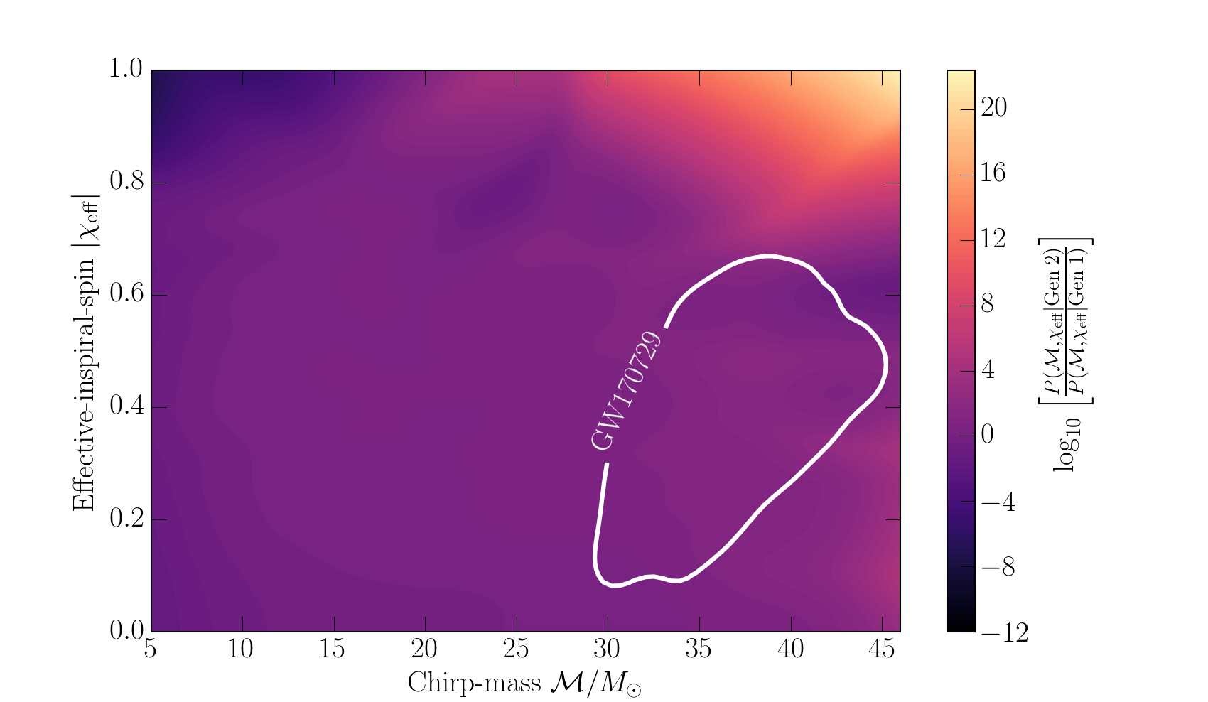
Relative likelihood of a binary black hole being second-generation versus first-generation for different values of the chirp mass and the magnitude of the effective inspiral spin. The white contour gives the 90% credible area for GW170729. Figure 1 of Kimball et al. (2019).

The plot above shows the relative probabilities. Yellow indicate chirp mass and effective inspiral spins which are more likely with second-generation systems, while dark purple indicates values more likely with first-generation systems.. The first thing I realised was my idea about the spin was off. We expect binaries with second-generation black holes to be formed dynamically. Following the first merger, the black hole wander around until it gets close enough to form a new binary with a new black hole. For dynamically formed binaries the spins should be randomly distributed. This means that there’s only a small probability of having a spin aligned with the orbital angular momentum as measured for GW170729. Most of the time, you’d measure an effective inspiral spin of around zero.

Since we don’t know exactly the chirp mass and effective inspiral spin for GW170729, we have to average over our uncertainty. That gives the ratio of the probability of observing GW170729 given a second-generation source, verses given a first-generation source. Using different inferred black hole populations (for example, ones inferred including and excluding GW170729), we find ratios of between 0.2 (meaning the first-generation origin is more likely) and 16 (meaning second generation is more likely). The results change significantly as the result is sensitive to the maximum mass of a black hole. If we include GW170729 in our population inference for first-generation systems, the maximum mass goes up, and it’s easier to explain the system as first-generation (as you’d expect).

Before you place your bets, there is one more piece to the calculation. We have calculated the relative probabilities of the observed properties assuming either first-generation black holes or a second-generation black hole, but we have not folded in the relative rates of mergers [bonus note]. We expect first-generation only binaries to be more common than ones containing second generation black holes. In simulations of globular clusters, at most about 20% of merging binaries are with second-generation black holes. For binaries not in an environment like a globular cluster (where there are lots of nearby black holes to grab), we expect the fraction of second-generation black holes in binaries to be basically zero. Therefore, on balance we have at best a weak preference for a second-generation black hole and most probably just two first-generation black holes in GW170729’s source, despite its large mass.

Verdict

What we have learnt from this calculation is that it seems that all of the first 10 binary black holes contain only first-generation black holes. It is safe to infer the properties of first-generation black holes from these observations. Detecting second-generation black holes requires knowledge of this distribution, and crucially if there is a maximum mass. As we get more detection, we’ll be able to pin this down. There is still a lot to learn about the full black hole family.

If you’d like to understand our calculation, the paper is extremely short. It is therefore an excellent paper to bring to journal club if you are a PhD student who forgot you were presenting this week…

arXiv: 1903.07813 [astro-ph.HE]
Journal: Research Notes of the AAS; 4(1):2; 2020 [bonus note]
Gizmodo story: The gravitational wave detectors are turning back on and we’re psyched
Theme music: Nice to see you!

Bonus notes

Useful papers

Back in 2017 two papers hit the arXiv [bonus bonus note] at pretty much the same time addressing the expected properties of second-generation black holes: Fishbach, Holz & Farr (2017), and Gerosa & Berti (2017). Both are nice reads.

I was asked how we could tell if the black holes we were seeing were themselves the results of mergers back in 2016 when I was giving a talk to the Carolian Astronomical Society. It was a good question. I explained about the masses and spins, but I didn’t think about how to actually do the analysis to infer if we had a merger. I now make a note to remember any questions I’m asked, as they can be good inspiration for projects!

Bayes factor and odds ratio

The quantity we work out in the paper is the Bayes factor for a second-generation system verses a first-generation one

$\displaystyle \frac{P(\mathrm{GW170729}|\mathrm{Gen\ 2})}{P(\mathrm{GW170729}|\mathrm{Gen\ 1})}$ .

What we want is the odds ratio

$\displaystyle \frac{P(\mathrm{Gen\ 2}|\mathrm{GW170729})}{P(\mathrm{Gen\ 1}|\mathrm{GW170729})}$ ,

which gives the betting odds for the two scenarios. The convert the Bayes factor into an odds ratio we need the prior odds

$\displaystyle \frac{P(\mathrm{Gen\ 2})}{P(\mathrm{Gen\ 1})}$ .

We’re currently working on a better way to fold these pieces together.

1000 words

As this was a quick calculation, we thought it would be a good paper to be a Research Note. Research Notes are limited to 1000 words, which is a tough limit. We carefully crafted the document, using as many word-saving measures (such as abbreviations), as we could. We made it to the limit by our counting, only to submit and find that we needed to share another 100 off! Fortunately, the arXiv [bonus bonus note] is more forgiving, so you can read our more relaxed (but still delightfully short) version there. It’s the one I’d recommend.

arXiv

For those reading who are not professional physicists, the arXiv (pronounced archive, as the X is really the Greek letter chi χ) is a preprint server. It where physicists can post version of their papers ahead of publication. This allows sharing of results earlier (both good as it can take a while to get a final published paper, and because you can get feedback before finalising a paper), and, vitally, for free. Most published papers require a subscription to read. Fine if you’re at a university, not so good otherwise. The arXiv allows anyone to read the latest research. Admittedly, you have to be careful, as not everything on the arXiv will make it through peer review, and not everyone will update their papers to reflect the published version. However, I think the arXiv is a very good thing™. There are few things I can think of which have benefited modern science as much. I would 100% support those behind the arXiv receiving a Nobel Prize, as I think it has had just as a significant impact on the development of the field as the discovery of dark matter, understanding nuclear fission, or deducing the composition of the Sun.

Dirichlet Process Gaussian-mixture model: An application to localizing coalescing binary neutron stars with gravitational-wave observations

August 10, 2018August 20, 2019 / CPLB / Leave a comment

Where do gravitational waves like GW170817 come from? Using our network of detectors, we cannot pinpoint a source, but we can make a good estimate—the amplitude of the signal tells us about the distance; the time delay between the signal arriving at different detectors, and relative amplitudes of the signal in different detectors tells us about the sky position (see the excellent video by Leo Singer below).

In this paper we look at full three-dimensional localization of gravitational-wave sources; we important a (rather cunning) technique from computer vision to construct a probability distribution for the source’s location, and then explore how well we could localise a set of simulated binary neutron stars. Knowing the source location enables lots of cool science. First, it aids direct follow-up observations with non-gravitational-wave observatories, searching for electromagnetic or neutrino counterparts. It’s especially helpful if you can cross-reference with galaxy catalogues, to find the most probable source locations (this technique was used to find the kilonova associated with GW170817). Even without finding a counterpart, knowing the most probable host galaxy helps us figure out how the source formed (have lots of stars been born recently, or are all the stars old?), and allows us measure the expansion of the Universe. Having a reliable technique to reconstruct source locations is useful!

This was a fun paper to write [bonus note]. I’m sure it will be valuable, both for showing how to perform this type of reconstruction of a multi-dimensional probability density, and for its implications for source localization and follow-up of gravitational-wave signals. I go into details of both below, first discussing our statistical model (this is a bit technical), then looking at our results for a set of binary neutron stars (which have implications for hunting for counterparts) .

Dirichlet process Gaussian mixture model

When we analyse gravitational-wave data to infer the source properties (location, masses, etc.), we map out parameter space with a set of samples: a list of points in the parameter space, with there being more around more probable locations and fewer in less probable locations. These samples encode everything about the probability distribution for the different parameters, we just need to extract it…

For our application, we want a nice smooth probability density. How do we convert a bunch of discrete samples to a smooth distribution? The simplest thing is to bin the samples. However, picking the right bin size is difficult, and becomes much harder in higher dimensions. Another popular option is to use kernel density estimation. This is better at ensuring smooth results, but you now have to worry about the size of your kernels.

Our approach is in essence to use a kernel density estimate, but to learn the size and position of the kernels (as well as the number) from the data as an extra layer of inference. The “Gaussian mixture model” part of the name refers to the kernels—we use several different Gaussians. The “Dirichlet process” part refers to how we assign their properties (their means and standard deviations). What I really like about this technique, as opposed to the usual rule-of-thumb approaches used for kernel density estimation, is that it is well justified from a theoretical point of view.

I hadn’t come across a Dirchlet process before. Section 2 of the paper is a walkthrough of how I built up an understanding of this mathematical object, and it contains lots of helpful references if you’d like to dig deeper.

In our application, you can think of the Dirichlet process as being a probability distribution for probability distributions. We want a probability distribution describing the source location. Given our samples, we infer what this looks like. We could put all the probability into one big Gaussian, or we could put it into lots of little Gaussians. The Gaussians could be wide or narrow or a mix. The Dirichlet distribution allows us to assign probabilities to each configuration of Gaussians; for example, if our samples are all in the northern hemisphere, we probably want Gaussians centred around there, rather than in the southern hemisphere.

With the resulting probability distribution for the source location, we can quickly evaluate it at a single point. This means we can rapidly produce a list of most probable source galaxies—extremely handy if you need to know where to point a telescope before a kilonova fades away (or someone else finds it).

Gravitational-wave localization

To verify our technique works, and develop an intuition for three-dimensional localizations, we used studied a set of simulated binary neutron star signals created for the First 2 Years trilogy of papers. This data set is well studied now, it illustrates performance it what we anticipated to be the first two observing runs of the advanced detectors, which turned out to be not too far from the truth. We have previously looked at three-dimensional localizations for these signals using a super rapid approximation.

The plots below show how well we could localise the sources of our binary neutron star sources. Specifically, the plots show the size of the volume which has a 90% probability of containing the source verses the signal-to-noise ratio (the loudness) of the signal. Typically, volumes are $10^4$ – $10^5~\mathrm{Mpc}^3$ , which is about $10^{68}$ – $10^{69}$ Olympic swimming pools. Such a volume would contain something like $100$ – $1000$ galaxies.

Localization volume as a function of signal-to-noise ratio. The top panel shows results for two-detector observations: the LIGO-Hanford and LIGO-Livingston (HL) network similar to in the first observing run, and the LIGO and Virgo (HLV) network similar to the second observing run. The bottom panel shows all observations for the HLV network including those with all three detectors which are colour coded by the fraction of the total signal-to-noise ratio from Virgo. In both panels, there are fiducial lines scaling inversely with the sixth power of the signal-to-noise ratio. Adapted from Fig. 4 of Del Pozzo et al. (2018).

Looking at the results in detail, we can learn a number of things

The localization volume is roughly inversely proportional to the sixth power of the signal-to-noise ratio [bonus note]. Loud signals are localized much better than quieter ones!
The localization dramatically improves when we have three-detector observations. The extra detector improves the sky localization, which reduces the localization volume.
To get the benefit of the extra detector, the source needs to be close enough that all the detectors could get a decent amount of the signal-to-noise ratio. In our case, Virgo is the least sensitive, and we see the the best localizations are when it has a fair share of the signal-to-noise ratio.
Considering the cases where we only have two detectors, localization volumes get bigger at a given signal-to-noise ration as the detectors get more sensitive. This is because we can detect sources at greater distances.

Putting all these bits together, I think in the future, when we have lots of detections, it would make most sense to prioritise following up the loudest signals. These are the best localised, and will also be the brightest since they are the closest, meaning there’s the greatest potential for actually finding a counterpart. As the sensitivity of the detectors improves, its only going to get more difficult to find a counterpart to a typical gravitational-wave signal, as sources will be further away and less well localized. However, having more sensitive detectors also means that we are more likely to have a really loud signal, which should be really well localized.

Left: Localization (yellow) with a network of two low-sensitivity detectors. The sky location is uncertain, but we know the source must be nearby. Right: Localization (green) with a network of three high-sensitivity detectors. We have good constraints on the source location, but it could now be at a much greater range of distances. Not to scale.

Using our localization volumes as a guide, you would only need to search one galaxy to find the true source in about 7% of cases with a three-detector network similar to at the end of our second observing run. Similarly, only ten would need to be searched in 23% of cases. It might be possible to get even better performance by considering which galaxies are most probable because they are the biggest or the most likely to produce merging binary neutron stars. This is definitely a good approach to follow.

Three-dimensional localization with galaxy catalgoue

Galaxies within the 90% credible volume of an example simulated source, colour coded by probability. The galaxies are from the GLADE Catalog; incompleteness in the plane of the Milky Way causes the missing wedge of galaxies. The true source location is marked by a cross [bonus note]. Part of Figure 5 of Del Pozzo et al. (2018).

arXiv: 1801.08009 [astro-ph.IM]
Journal: Monthly Notices of the Royal Astronomical Society; 479(1):601–614; 2018
Code: 3d_volume
Buzzword bingo: Interdisciplinary (we worked with computer scientist Tom Haines); machine learning (the inference involving our Dirichlet process Gaussian mixture model); multimessenger astronomy (as our results are useful for following up gravitational-wave signals in the search for counterparts)

Bonus notes

Writing

We started writing this paper back before the first observing run of Advanced LIGO. We had a pretty complete draft on Friday 11 September 2015. We just needed to gather together a few extra numbers and polish up the figures and we’d be done! At 10:50 am on Monday 14 September 2015, we made our first detection of gravitational waves. The paper was put on hold. The pace of discoveries over the coming years meant we never quite found enough time to get it together—I’ve rewritten the introduction a dozen times. It’s extremely satisfying to have it done. This is a shame, as it meant that this study came out much later than our other three-dimensional localization study. The delay has the advantage of justifying one of my favourite acknowledgement sections.

Sixth power

We find that the localization volume $\Delta V$ is inversely proportional to the sixth power of the signal-to-noise ration $\varrho$ . This is what you would expect. The localization volume depends upon the angular uncertainty on the sky $\Delta \Omega$ , the distance to the source $D$ , and the distance uncertainty $\Delta D$ ,

$\Delta V \sim D^2 \Delta \Omega \Delta D$ .

Typically, the uncertainty on a parameter (like the masses) scales inversely with the signal-to-noise ratio. This is the case for the logarithm of the distance, which means

$\displaystyle \frac{\Delta D}{D} \propto \varrho^{-1}$ .

The uncertainty in the sky location (being two dimensional) scales inversely with the square of the signal-to-noise ration,

$\Delta \Omega \propto \varrho^{-2}$ .

The signal-to-noise ratio itself is inversely proportional to the distance to the source (sources further way are quieter. Therefore, putting everything together gives

$\Delta V \propto \varrho^{-6}$ .

Treasure

We all know that treasure is marked by a cross. In the case of a binary neutron star merger, dense material ejected from the neutron stars will decay to heavy elements like gold and platinum, so there is definitely a lot of treasure at the source location.

Puzzle procrastination: perplexing probabilities part II

February 27, 2015 / CPLB / Leave a comment

A while ago I set some probability puzzles. If you’ve not yet pondered them, give them a whirl now. It’s OK, I’ll wait… All done? Final answer?

1 Girls, boys and doughnuts

We know that Laura has two children. There are four possibilities: two girls ( $\mathrm{GG}$ ), a boy and a girl ( $\mathrm{BG}$ ), a girl and a boy ( $\mathrm{GB}$ ) and two boys ( $\mathrm{BB}$ ). The probability of having a boy is almost identical to having a girl, so let’s keep things simple and assume that all four options have equal probability.

In this case, (i) the probability of having two girls is $P(\mathrm{GG}) = 1/4$ ; (ii) the probability of having a boy and a girl is $P(\mathrm{B,\,G}) = P(\mathrm{BG}) + P(\mathrm{GB}) = 1/2$ , and (iii) the probability of having two boys is $P(\mathrm{BB}) = 1/4$ .

After meeting Laura’s daughter Lucy, we know she doesn’t have two boys. What are the probabilities now? There are three options left ( $\mathrm{GG}$ , $\mathrm{GB}$ and $\mathrm{BG}$ ), but they are not all equally likely. We’ve discussed a similar problem before (it involved water balloons). You can work out the probabilities using Bayes’ Theorem, but let’s see if we can get away without using any maths more complicated than addition. Lucy could either be the elder or the younger child, each is equally likely. There must be four possible outcomes: Lucy and then another girl ( $\mathrm{LG}$ ), another girl and then Lucy ( $\mathrm{GL}$ ), Lucy and then a boy ( $\mathrm{LB}$ ) or a boy and then Lucy ( $\mathrm{BL}$ ). Since the sex of children are not linked (if we ignore the possibility of identical twins), each of these are equally probable. Therefore, (i) $P(\mathrm{GG}) = P(\mathrm{LG}) + P(\mathrm{GL}) = 1/2$ ; (ii) $P(\mathrm{B,\,G}) = P(\mathrm{LB}) + P(\mathrm{BL}) = 1/2$ , and (iii) $P(\mathrm{BB}) = 0$ . We have ruled out one possibility, and changed the probability having two girls.

If we learn that Lucy is the eldest, then we are left with two options, $\mathrm{LG}$ and $\mathrm{LB}$ . This means (i) $P(\mathrm{GG}) = P(\mathrm{LG}) = 1/2$ ; (ii) $P(\mathrm{B,\,G}) = P(\mathrm{LB}) = 1/2$ , and (iii) $P(\mathrm{BB}) = 0$ . The probabilities haven’t changed! This is because the order of birth doesn’t influence the probability of being a boy or a girl.

Hopefully that all makes sense so far. Now let’s move on to Laura’s secret society for people who have two children of which at least one is a girl. There are three possibilities for the children: $\mathrm{GG}$ , $\mathrm{BG}$ or $\mathrm{GB}$ . This time, all three are equally likely as we are just selecting them equally from the total population. Families with two children are equally likely to have each of the four combinations, but those with $\mathrm{BB}$ are turned away at the door, leaving an equal mix of the other three. Hence, (i) $P(\mathrm{GG}) = 1/3$ ; (ii) $P(\mathrm{B,\,G}) = P(\mathrm{BG}) + P(\mathrm{GB}) = 2/3$ , and (iii) $P(\mathrm{BB}) = 0$ .

The probabilities are different in this final case than for Laura’s family! This is because of the difference in the way we picked are sample. With Laura, we knew she had two children, the probability that she would have a daughter with her depends upon how many daughters she has. It’s more likely that she’d have a daughter with her if she has two, than one (or zero). If we’re picking families with at least one girl at random, things are different. This has confused enough people to be known as the boy or girl paradox. However, if you’re careful in writing things down, it’s not too tricky to work things out.

2 Do or do-nut

You’re eating doughnuts, and trying to avoid the one flavour you don’t like. After eating six of twenty-four you’ve not encountered it. The other guests have eaten twelve, but that doesn’t tell you if they’ve eaten it. All you know is that it’s not in the six you’ve eaten, hence it must be one of the other eighteen. The probability that one of the twelve that the others have eaten is the nemesis doughnut is $P(\mathrm{eaten}) = 12/18 = 2/3$ . Hence, the probability it is left is $P(\mathrm{left}) = 1 - P(\mathrm{eaten}) = 1/3$ . Since there are six doughnuts left, the probability you’ll pick the nemesis doughnut next is $P(\mathrm{next}) = P(\mathrm{left}) \times 1/6 = 1/18$ . Equally, you could have figured that out by realising that it’s equally probable that the nemesis doughnut is any of the eighteen that you’ve not eaten.

When twelve have been eaten, Lucy takes one doughnut to feed the birds. You all continue eating until there are four left. At this point, no-one has eaten that one doughnut. There are two possible options: either it’s still lurking or it’s been fed to the birds. Because we didn’t get to use it in the first part, I’ll use Bayes’ Theorem to work out the probabilities for both options.

The probability that Lucy luckily picked that one doughnut to feed to the birds is $P(\mathrm{lucky}) = 1/12$ , the probability that she unluckily picked a different flavour is $P(\mathrm{unlucky}) = 1 - P(\mathrm{lucky}) = 11/12$ . If we were lucky, the probability that we managed to get down to there being four left is $P(\mathrm{four}|\mathrm{lucky}) = 1$ , we were guaranteed not to eat it! If we were unlucky, that the bad one is amongst the remaining eleven, the probability of getting down to four is $P(\mathrm{four}|\mathrm{unlucky}) = 4/11$ . The total probability of getting down to four is

$P(\mathrm{four}) = P(\mathrm{four}|\mathrm{lucky})P(\mathrm{lucky}) + P(\mathrm{four}|\mathrm{unlucky})P(\mathrm{unlucky})$ .

Substituting in gives

$\displaystyle P(\mathrm{four}) = 1 \times \frac{1}{12} + \frac{4}{11} \times \frac{11}{12} = \frac{5}{12}$ .

The probability that the doughnut is not left is when there are four left is

$\displaystyle P(\mathrm{lucky}|\mathrm{four}) = \frac{P(\mathrm{four}|\mathrm{lucky})P(\mathrm{lucky})}{P(\mathrm{four})}$ ,

putting in the numbers gives

$\displaystyle P(\mathrm{lucky}|\mathrm{four}) = 1 \times \frac{1}{12} \times \frac{12}{5} = \frac{1}{5}$ .

The probability that it’s left must be

$\displaystyle P(\mathrm{unlucky}|\mathrm{four}) = \frac{4}{5}$ .

We could’ve worked this out more quickly by realised that there are five doughnuts that could potential be the one: the four left and the one fed to the birds. Each one is equally probable, so that gives $P(\mathrm{lucky}|\mathrm{four}) = 1/5$ and $P(\mathrm{unlucky}|\mathrm{four}) = 4/5$ .

If you take one doughnut each, one after another, does it matter when you pick? You have an equal probability of each being the one. The probability that it’s the first is

$\displaystyle P(\mathrm{first}) = \frac{1}{4} \times P(\mathrm{unlucky}|\mathrm{four}) = \frac{1}{5}$ ;

the probability that it’s the second is

$\displaystyle P(\mathrm{second}) = \frac{1}{3} \times \frac{3}{4} \times P(\mathrm{unlucky}|\mathrm{four}) = \frac{1}{5}$ ;

the probability that it’s the third is

$\displaystyle P(\mathrm{third}) = \frac{1}{2} \times \frac{2}{3} \times \frac{3}{4} \times P(\mathrm{unlucky}|\mathrm{four}) = \frac{1}{5}$ ,

and the probability that it’s the fourth (last) is

$\displaystyle P(\mathrm{third}) = 1 \times \frac{1}{2} \times \frac{2}{3} \times \frac{3}{4} \times P(\mathrm{unlucky}|\mathrm{four}) = \frac{1}{5}$ .

That doesn’t necessarily mean it doesn’t matter when you pick though! That really depends how you feel when taking an uncertain bite, how much you value the knowledge that you can safely eat your doughnut, and how you’d feel about skipping your doughnut rather than eating one you hate.

Puzzle procrastination: perplexing probabilities

November 2, 2014February 27, 2015 / CPLB / Leave a comment

I enjoy pondering over puzzles. Figuring out correct probabilities can be confusing, but it is a good exercise to practise logical reasoning. Previously, we have seen how to update probabilities when given new information; let’s see if we use this to solve some puzzles!

1 Girls, boys and doughnuts

As an example, we’ve previously calculated the probabilities for the boy–girl distribution of our office-mate Iris’ children. Let’s imagine that we’ve popped over to Iris’ for doughnuts (this time while her children are out), and there we meet her sister Laura. Laura tells us that she has two children. What are the probabilities that Laura has: (i) two girls, (ii) a girl and a boy, or (iii) two boys?

It turns out that Laura has one of her children with her. After you finish your second doughnut (a chocolatey, custardy one), Laura introduces you to her daughter Lucy. Lucy loves LEGO, but that is unimportant for the current discussion. How does Lucy being a girl change the probabilities?

While you are finishing up your third doughnut (with plum and apple jam), you discover that Lucy is the eldest child. What are the probabilities now—have they changed?

Laura is a member of an extremely selective club for mothers with two children of which at least one is a girl. They might fight crime at the weekends, Laura gets a little evasive about what they actually do. What are the probabilities that a random member of this club has (i) two girls, (ii) a girl and a boy, or (iii) two boys?

The answers to similar questions have been the subject to lots of argument, even though they aren’t about anything too complicated. If you figure out the answers, you might see how the way you phrase the question is important.

2 Do or do-nut

You are continuing to munch through the doughnuts at Iris’. You are working your way through a box of 24. There is one of each flavour and you know there is one you do not like (which we won’t mention for liable reasons). There’s no way of telling what flavour a doughnut is before biting into it. You have now eaten six, not one of which was the bad one. The others have eaten twelve between them. What is the probability that your nemesis doughnut is left? What is the probability that you will pick it up next?

You continue munching, as do the others. You discover that Iris, Laura and Lucy all hate the same flavour that you do, but that none of them have eaten it. There are now just four doughnuts left. Lucy admits that she did take one of the doughnuts to feed the birds in the garden (although they didn’t actually eat it as they are trying to stick to a balanced diet). She took the doughnut while there were still 12 left. What is the probability that the accursed flavour is still lurking amongst the final four?

You are agree to take one each, one after another. Does it matter when you pick yours?

Happy pondering! I shall post the solutions later.

An introduction to probability: Inference and learning from data

October 18, 2014February 7, 2015 / CPLB / Leave a comment

Probabilities are a way of quantifying your degree of belief. The more confident you are that something is true, the larger the probability assigned to it, with 1 used for absolute certainty and 0 used for complete impossibility. When you get new information that updates your knowledge, you should revise your probabilities. This is what we do all the time in science: we perform an experiment and use our results to update what we believe is true. In this post, I’ll explain how to update your probabilities, just as Sherlock Holmes updates his suspicions after uncovering new evidence.

Taking an umbrella

Imagine that you are a hard-working PhD student and you have been working late in your windowless office. Having finally finished analysing your data, you decide it’s about time to go home. You’ve been trapped inside so long that you no idea what the weather is like outside: should you take your umbrella with you? What is the probability that it is raining? This will depend upon where you are, what time of year it is, and so on. I did my PhD in Cambridge, which is one of the driest places in England, so I’d be confident that I wouldn’t need one. We’ll assume that you’re somewhere it doesn’t rain most of the time too, so at any random time you probably wouldn’t need an umbrella. Just as you are about to leave, your office-mate Iris comes in dripping wet. Do you reconsider taking that umbrella? We’re still not certain that it’s raining outside (it could have stopped, or Iris could’ve just been in a massive water-balloon fight), but it’s now more probable that it is raining. I’d take the umbrella. When we get outside, we can finally check the weather, and be pretty certain if it’s raining or not (maybe not entirely certain as, after plotting that many graphs, we could be hallucinating).

In this story we get two new pieces of information: that newly-arrived Iris is soaked, and what we experience when we get outside. Both of these cause us to update our probability that it is raining. What we learn doesn’t influence whether it is raining or not, just what we believe regarding if it is raining. Some people worry that probabilities should be some statement of absolute truth, and so because we changed our probability of it raining after seeing that our office-mate is wet, there should be some causal link between office-mates and the weather. We’re not saying that (you can’t control the weather by tipping a bucket of water over your office-mate), our probabilities just reflect what we believe. Hopefully you can imagine how your own belief that it is raining would change throughout the story, we’ll now discuss how to put this on a mathematical footing.

Bayes’ theorem

We’re going to venture into using some maths now, but it’s not too serious. You might like to skip to the example below if you prefer to see demonstrations first. I’ll use $P(A)$ to mean the probability of $A$ . A joint probability describes the probability of two (or more things), so we have $P(A, B)$ as the probability that both $A$ and $B$ happen. The probability that $A$ happens given that $B$ happens is the conditional probability $P(A|B)$ . Consider the the joint probability of $A$ and $B$ : we want both to happen. We could construct this in a couple of ways. First we could imagine that $A$ happens, and then $B$ . In this case we build up the joint probability of both by working out the probability that $A$ happens and then the probability $B$ happens given $A$ . Putting that in equation form

$P(A,B) = P(A)P(B|A)$ .

Alternatively, we could have $B$ first and then $A$ . This gives us a similar result of

$P(A,B) = P(B)P(A|B)$ .

Both of our equations give the same result. (We’ve checked this before). If we put the two together then

$P(B|A)P(A) = P(A|B)P(B)$ .

Now we divide both sides by $P(A)$ and bam:

$\displaystyle P(B|A) = \frac{P(A|B)P(B)}{P(A)}$ ,

this is Bayes’ theorem. I think the Reverend Bayes did rather well to get a theorem named after him for noting something that is true and then rearranging! We use Bayes’ theorem to update our probabilities.

Usually, when doing inference (when trying to learn from some evidence), we have some data (that our office-mate is damp) and we want to work out the probability of our hypothesis (that it’s raining). We want to calculate $P(\mathrm{hypothesis}|\mathrm{data})$ . We normally have a model that can predict how likely it would be to observe that data if our hypothesis is true, so we know $P(\mathrm{data}|\mathrm{hypothesis})$ , so we just need to convert between the two. This is known as the inverse problem.

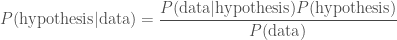
We can do this using Bayes’ theorem

$\displaystyle P(\mathrm{hypothesis}|\mathrm{data}) = \frac{P(\mathrm{data}|\mathrm{hypothesis})P(\mathrm{hypothesis})}{P(\mathrm{data})}$ .

In this context, we give names to each of the probabilities (to make things sound extra fancy): $P(\mathrm{hypothesis}|\mathrm{data})$ is the posterior, because it’s what we get at the end; $P(\mathrm{data}|\mathrm{hypothesis})$ is the likelihood, it’s what you may remember calculating in statistics classes; $P(\mathrm{hypothesis})$ is the prior, because it’s what we believed about our hypothesis before we got the data, and $P(\mathrm{data})$ is the evidence. If ever you hear of someone doing something in a Bayesian way, it just means they are using the formula above. I think it’s rather silly to point this out, as it’s really the only logical way to do science, but people like to put “Bayesian” in the title of their papers as it sounds cool.

Whenever you get some new information, some new data, you should update your belief in your hypothesis using the above. The prior is what you believed about hypothesis before, and the posterior is what you believe after (you’ll use this posterior as your prior next time you learn something new). There are a couple of examples below, but before we get there I will take a moment to discuss priors.

About priors: what we already know

There have been many philosophical arguments about the use of priors in science. People worry that what you believe affects the results of science. Surely science should be above such things: it should be about truth, and should not be subjective! Sadly, this is not the case. Using Bayes’ theorem is the only logical thing to do. You can’t calculate a probability of what you believe after you get some data unless you know what you believed beforehand. If this makes you unhappy, just remember that when we changed our probability for it being raining outside, it didn’t change whether it was raining or not. If two different people use two different priors they can get two different results, but that’s OK, because they know different things, and so they should expect different things to happen.

To try to convince yourself that priors are necessary, consider the case that you are Sherlock Holmes (one of the modern versions), and you are trying to solve a bank robbery. There is a witness who saw the getaway, and they can remember what they saw with 99% accuracy (this gives the likelihood). If they say the getaway vehicle was a white transit van, do you believe them? What if they say it was a blue unicorn? In both cases the witness is the same, the likelihood is the same, but one is much more believable than the other. My prior that the getaway vehicle is a transit van is much greater than my prior for a blue unicorn: the latter can’t carry nearly as many bags of loot, and so is a silly choice.

If you find that changing your prior (to something else sensible) significantly changes your results, this just means that your data don’t tell you much. Imagine that you checked the weather forecast before leaving the office and it said “cloudy with 0–100% chance of precipitation”. You basically believe the same thing before and after. This really means that you need more (or better) data. I’ll talk about some good ways of calculating priors in the future.

Solving the inverse problem

Example 1: Doughnut allergy

We shall now attempt to use Bayes’ theorem to calculate some posterior probabilities. First, let’s consider a worrying situation. Imagine there is a rare genetic disease that makes you allergic to doughnuts. One in a million people have this disease, that only manifests later in life. You have tested positive. The test is 99% successful at detecting the disease if it is present, and returns a false positive (when you don’t have the disease) 1% of the time. How worried should you be? Let’s work out the probability of having the disease given that you tested positive

$\displaystyle P(\mathrm{allergy}|\mathrm{positive}) = \frac{P(\mathrm{positive}|\mathrm{allergy})P(\mathrm{allergy})}{P(\mathrm{positive})}$ .

Our prior for having the disease is given by how common it is, $P(\mathrm{allergy}) = 10^{-6}$ . The prior probability of not having the disease is $P(\mathrm{no\: allergy}) = 1 - P(\mathrm{allergy})$ . The likelihood of our positive result is $P(\mathrm{positive}|\mathrm{allergy}) = 0.99$ , which seems worrying. The evidence, the total probability of testing positive $P(\mathrm{positive})$ is found by adding the probability of a true positive and a false positive

$P(\mathrm{positive}) = P(\mathrm{positive}|\mathrm{allergy})P(\mathrm{allergy}) + P(\mathrm{positive}|\mathrm{no\: allergy})P(\mathrm{no\: allergy})$ .

The probability of a false positive is $P(\mathrm{positive}|\mathrm{no\: allergy}) = 0.01$ . We thus have everything we need. Substituting everything in, gives

$\displaystyle P(\mathrm{allergy}|\mathrm{positive}) = \frac{0.99 \times 10^{-6}}{0.99 \times 10^{-6} + 0.01 \times (1 - 10^{-6})} = 9.899 \times 10^{-5}$ .

Even after testing positive, you still only have about a one in ten thousand chance of having the allergy. While it is more likely that you have the allergy than a random member of the public, it’s still overwhelmingly probable that you’ll be fine continuing to eat doughnuts. Hurray!

Doughnut love: probably fine.

Example 2: Boys, girls and water balloons

Second, imagine that Iris has three children. You know she has a boy and a girl, but you don’t know if she has two boys or two girls. You pop around for doughnuts one afternoon, and a girl opens the door. She is holding a large water balloon. What’s the probability that Iris has two girls? We want to calculate the posterior

$\displaystyle P(\mathrm{two\: girls}|\mathrm{girl\:at\:door}) = \frac{P(\mathrm{girl\:at\:door}|\mathrm{two\: girls})P(\mathrm{two\: girls})}{P(\mathrm{girl\:at\:door})}$ .

As a prior, we’d expect boys and girls to be equally common, so $P(\mathrm{two\: girls}) = P(\mathrm{two\: boys}) = 1/2$ . If we assume that it is equally likely that any one of the children opened the door, then the likelihood that one of the girls did so when their are two of them is $P(\mathrm{girl\:at\:door}|\mathrm{two\: girls}) = 2/3$ . Similarly, if there were two boys, the probability of a girl answering the door is $P(\mathrm{girl\:at\:door}|\mathrm{two\: boys}) = 1/3$ . The evidence, the total probability of a girl being at the door is

$P(\mathrm{girl\:at\:door}) =P(\mathrm{girl\:at\:door}|\mathrm{two\: girls})P(\mathrm{two\: girls}) +P(\mathrm{girl\:at\:door}|\mathrm{two\: boys}) P(\mathrm{two\: boys})$ .

Using all of these,

$\displaystyle P(\mathrm{two\: girls}|\mathrm{girl\:at\:door}) = \frac{(2/3)(1/2)}{(2/3)(1/2) + (1/3)(1/2)} = \frac{2}{3}$ .

Even though we already knew there was at least one girl, seeing a girl first makes it much more likely that the Iris has two daughters. Whether or not you end up soaked is a different question.

Example 3: Fudge!

Finally, we shall return to the case of Ted and his overconsumption of fudge. Ted claims to have eaten a lethal dose of fudge. Given that he is alive to tell the anecdote, what is the probability that he actually ate the fudge? Here, our data is that Ted is alive, and our hypothesis is that he did eat the fudge. We have

$\displaystyle P(\mathrm{fudge}|\mathrm{survive}) = \frac{P(\mathrm{survive}|\mathrm{fudge})P(\mathrm{fudge})}{P(\mathrm{survive})}$ .

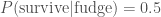
This is a case where our prior, the probability that he would eat a lethal dose of fudge $P(\mathrm{fudge})$ , makes a difference. We know the probability of surviving the fatal dose is $P(\mathrm{survive}|\mathrm{fudge}) = 0.5$ . The evidence, the total probability of surviving $P(\mathrm{survive})$ , is calculated by considering the two possible sequence of events: either Ted ate the fudge and survived or he didn’t eat the fudge and survived

$P(\mathrm{survive}) = P(\mathrm{survive}|\mathrm{fudge})P(\mathrm{fudge}) + P(\mathrm{survive}|\mathrm{no\: fudge})P(\mathrm{no\: fudge})$ .

We’ll assume if he didn’t eat the fudge he is guaranteed to be alive, $P(\mathrm{survive}| \mathrm{no\: fudge}) = 1$ . Since Ted either ate the fudge or he didn’t $P(\mathrm{fudge}) + P(\mathrm{no\: fudge}) = 1$ . Therefore,

$P(\mathrm{survive}) = 0.5 P(\mathrm{fudge}) + [1 - P(\mathrm{fudge})] = 1 - 0.5 P(\mathrm{fudge})$ .

This gives us a posterior

$\displaystyle P(\mathrm{fudge}|\mathrm{survive}) = \frac{0.5 P(\mathrm{fudge})}{1 - 0.5 P(\mathrm{fudge})}$ .

We just need to decide on a suitable prior.

If we believe Ted could never possibly lie, then he must have eaten that fudge and $P(\mathrm{fudge}) = 1$ . In this case,

$\displaystyle P(\mathrm{fudge}|\mathrm{survive}) = \frac{0.5}{1 - 0.5} = 1$ .

Since we started being absolutely sure, we end up being absolutely sure: nothing could have changed our mind! This is a poor prior: it is too strong, we are being closed-minded. If you are closed-minded you can never learn anything new.

If we don’t know who Ted is, what fudge is, or the ease of consuming a lethal dose, then we might assume an equal prior on eating the fudge and not eating the fudge, $P(\mathrm{fudge}) = 0.5$ . In this case we are in a state of ignorance. Our posterior is

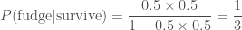
$\displaystyle P(\mathrm{fudge}|\mathrm{survive}) = \frac{0.5 \times 0.5}{1 - 0.5 \times 0.5} = \frac{1}{3}$ .

Even though we know nothing, we conclude that it’s more probable that the Ted did not eat the fudge. In fact, it’s twice as probable that he didn’t eat the fudge than he did as $P(\mathrm{no\: fudge}|\mathrm{survive}) = 1 -P(\mathrm{fudge}|\mathrm{survive}) = 2/3$ .

In reality, I think that it’s extremely improbable anyone could consume a lethal dose of fudge. I’m fairly certain that your body tries to protect you from such stupidity by expelling the fudge from your system before such a point. However, I will concede that it is not impossible. I want to assign a small probability to $P(\mathrm{fudge})$ . I don’t know if this should be one in a thousand, one in a million or one in a billion, but let’s just say it is some small value $p$ . Then

$\displaystyle P(\mathrm{fudge}|\mathrm{survive}) = \frac{0.5 p}{1 - 0.5 p} \approx 0.5 p$ .

as the denominator is approximately one. Whatever small probability I pick, it is half as probable that Ted ate the fudge.

I would assign a much higher probability to Mr. Impossible being able to eat that much fudge than Ted.

While it might not be too satisfying that we can’t come up with incontrovertible proof that Ted didn’t eat the fudge, we might be able to shut him up by telling him that even someone who knows nothing would think his story is unlikely, and that we will need much stronger evidence before we can overcome our prior.

Homework example: Monty Hall

You now have all the tools necessary to tackle the Monty Hall problem, one of the most famous probability puzzles:

You are on a game show and are given the choice of three doors. Behind one is a car (a Lincoln Continental), but behind the others are goats (which you don’t want). You pick a door. The host, who knows what is behind the doors, opens another door to reveal goat. They then offer you the chance to switch doors. Should you stick with your current door or not? — Monty Hall problem

You should be able to work out the probability of winning the prize by switching and sticking. You can’t guarantee you win, but you can maximise your chances.

Summary

Whenever you encounter new evidence, you should revise how probable you think things are. This is true in science, where we perform experiments to test hypotheses; it is true when trying to solve a mystery using evidence, or trying to avoid getting a goat on a game show. Bayes’ theorem is used to update probabilities. Although Bayes’ theorem itself is quite simple, calculating likelihoods, priors and evidences for use in it can be difficult. I hope to return to all these topics in the future.

An introduction to probability: Great expectations

August 16, 2014October 25, 2014 / CPLB / Leave a comment

We use probabilities a lot in science. Previously, I introduced the concept of probabilities, here I’ll explain the concept of expectation and averages. Expectation and average values are one of the most useful statistics that we can construct from a probability distribution. This post contains a traces of calculus, but is peanut free.

Expectations

Imagine that we have a discrete set of numeric outcomes, such as the number from rolling a die. We’ll label these as $x_1$ , $x_2$ , etc., or as $x_i$ where the subscript $i$ is used as shorthand to indicate any of the possible outcomes. The probability of the numeric value being a particular $x_i$ is given by $P(x_i)$ . For rolling our dice, the outcomes are one to six ( $x_1 =1$ , $x_2 = 2$ , etc.) and the probabilities are

$\displaystyle P(1) = P(2) = P(3) = P(4) = P(5) = P(6) = \frac{1}{6}$ .

The expectation value is the sum of all the possible outcomes multiplied by their respective probabilities,

$\displaystyle \langle x \rangle = \sum_i x_i P(x_i)$ ,

where $\sum_i$ means sum over all values of $i$ (over all outcomes). The expectation value for rolling a die is

$\displaystyle \langle x \rangle = 1 \times P(1) + 2 \times P(2) + 3 \times P(3) + 4 \times P(4) + 5 \times P(5) + 6 \times P(6) = \frac{7}{2}$ .

The expectation value of a distribution is its average, the value you’d expect after many (infinite) repetitions. (Of course this is possible in reality—you’d certainly get RSI—but it is useful for keeping statisticians out of mischief).

For a continuous distribution, the expectation value is given by

$\displaystyle \langle x \rangle = \int x p(x) \, \mathrm{d} x$ ,

where $p(x)$ is the probability density function.

You can use the expectation value to guide predictions for the outcome. You can never predict with complete accuracy (unless there is only one possible outcome), but you can use knowledge of the probabilities of the various outcomes the inform your predictions.

Imagine that after buying a large quantity of fudge, for entirely innocent reasons, the owner offers you the chance to play double-or-nothing—you’ll either pay double the bill or nothing, based on some random event—should you play? Obviously, this depends upon the probability of winning. Let’s say that the probability of winning is $p$ and find out how high it needs to be to be worthwhile. We can use the expectation value to calculate how much we should expect to pay, if this is less than the bill as it stands, it’s worth giving it a go, if the expectation value is larger than the original bill, we should expect to pay more (and so probably shouldn’t play). The expectation value is

$\displaystyle \langle x \rangle = 0 \times (1 - p) + 2 \times p = 2 p$ ,

where I’m working in terms of unified fudge currency, which, shockingly, is accepted in very few shops, but has the nice property that your fudge bill is always 1. Anyhow, if $\langle x \rangle$ is less than one, so if $p < 0.5$ , it’s worth playing. If we were tossing a (fair) coin, we’d expect to come out even, if we had to roll a six, we’d expect to pay more.

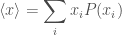
The expectation value is the equivalent of the mean. This is the average that people usually think of first. If you have a set of numeric results, you calculate the mean by adding up all or your results and dividing by the total number of results $N$ . Imagine each outcome $x_i$ occurs $n_i$ times, then the mean is

$\displaystyle \bar{x} = \sum_i x_i \frac{n_i}{N}$ .

We can estimate the probability of each outcome as $P(x_i) = n_i/N$ so that $\bar{x} = \langle x \rangle$ .

Median and mode

Aside from the mean there are two other commonly used averages, the median and the mode. These aren’t quite as commonly used, despite sounding friendlier. With a set of numeric results, the median is the middle result and the mode is the most common result. We can define equivalents for both when dealing with probability distributions.

To calculate the median we find the value where the total probability of being smaller (or bigger) than it is a half: $P(x < x_\mathrm{med}) = 0.5$ . This can be done by adding up probabilities until you get a half

$\displaystyle \sum_{x_i \, \leq \, x_\mathrm{med} } P(x_i) = 0.5$ .

For a continuous distribution this becomes

$\displaystyle \int_{x_\mathrm{low}}^{x_\mathrm{med}} p(x) \, \mathrm{d}x = 0.5$ ,

where $x_\mathrm{low}$ is the lower limit of the distribution. (That’s all the calculus out of the way now, so if you’re not a fan you can relax). The LD₅₀ lethal dose is a median. The median is effectively the middle of the distribution, the point at which you’re equally likely to be higher or lower.

The median is often used as it is not as sensitive as the mean to a few outlying results which are far from the typical values.

The mode is the value with the largest probability, the most probable outcome

$\displaystyle P(x_\mathrm{mode}) = \max P(x_i)$ .

For a continuous distribution, it is the point which maximises the probability density function

$\displaystyle p(x_\mathrm{mode}) = \max p(x)$ .

The modal value is the most probable outcome, the most likely result, the one to bet on if you only have one chance.

Education matters

Every so often, some official, usually an education minister, says something about wanting more than half of students to be above average. This results in much mocking, although seemingly little rise in the standards for education ministers. Having discussed averages ourselves, we can now see if it’s entirely fair to pick on these poor MPs.

The first line of defence, is that we should probably specify the distribution we’ve averaging. It may well be that they actually meant the average bear. It’s a sad truth that bears perform badly in formal education. Many blame the unfortunate stereotyping resulting from Winnie the Pooh. It might make sense to compare with performance in the past to see if standards are improving. We could imagine that taking the average from the 1400s would indeed show some improvement. For argument’s sake, let’s say that we are indeed talking about the average over this year’s students.

If the average we were talking about was the median, then it would be impossible for more (or fewer) than half of students to do better than average. In the case, it is entirely fair to mock the minister, and possibly to introduce them to the average bear. In this case, a mean bear.

If we were referring to the mode, then it is quite simple for more than half of the students to do better than this. To achieve this we just need a bottom-heavy distribution, a set of results where the most likely outcome is low, but most students do better than this. We might want to question an education system where the aim is to have a large number of students doing poorly though!

Finally, there is the mean; to use the mean, we first have to decide if we have a sensible if we are averaging a sensible quantity. For education performance this normally means exam results. Let’s sidestep the issue of if we want to reduce the output of the education system down to a single number, and consider the properties we want in order to take a sensible average. We want the results to be numeric (check); to be ordered, such that high is good and low is bad (or vice versa) so 42 is better than 41 but not as good as 43 and so on (check), and to be on a linear scale. The last criterion means that performance is directly proportional to the mark: a mark twice as big is twice as good. Most exams I’ve encountered are not like this, but I can imagine that it is possible to define a mark scheme this way. Let’s keep imagining, and assume things are sensible (and perhaps think about kittens and rainbows too… ).

We can construct a distribution where over half of students perform better than the mean. In this case we’d really need a long tail: a few students doing really very poorly. In this case, these few outliers are enough to skew the mean and make everyone else look better by comparison. This might be better than the modal case where we had a glut of students doing badly, as now we can have lots doing nicely. However, it also means that there are a few students who are totally failed by the system (perhaps growing up to become a minister for education), which is sad.

In summary, it is possible to have more than 50% of students performing above average, assuming that we are not using the median. It’s therefore unfair to heckle officials with claims of innumeracy. However, for these targets to be met requires lots of students to do badly. This seems like a poor goal. It’s probably better to try to aim for a more sensible distribution with about half of students performing above average, just like you’d expect.

An introduction to probability: Leaving nothing to chance

August 9, 2014October 25, 2014 / CPLB / Leave a comment

Probabilities and science

Understanding probabilities is important in science. Once you’ve done an experiment, you need to be able to extract from your data information about your theory. Only rarely do you get a simple yes or no: most of the time you have to work with probabilities to quantify your degree of certainty. I’ll (probably) be writing about probabilities in connection with my research, so I thought it would be useful to introduce some of the concepts.

I’ll be writing a series of posts, hopefully going through from the basics to the limits of my understanding. We’ll begin with introducing the concept of probability. There’s a little bit of calculus, but you can skip that without effecting the rest, just remember you can’t grow up to be big and strong if you don’t finish your calculus.

What is a probability?

A probability describes the degree of belief that you have in a proposition. We talk about probabilities quite intuitively: there are some angry-looking, dark clouds overhead and I’ve just lit the barbecue, so it’s probably going to rain; it’s more likely that United will win this year’s sportsball league than Rovers, or it’s more credible that Ted is exaggerating in his anecdote than he actually ate that much fudge…

We formalise the concept of a probability, so that it can be used in calculations, by assigning them numerical values (not by making them wear a bow-tie, although that is obviously cool). Conventionally, we use 0 for impossible, 1 for certain and the range in between for intermediate probabilities. For example, if we were tossing a coin, we might expect it to be heads half the time, hence the probability of heads is $P(\mathrm{head}) = 1/2$ , or if rolling a die, the probability of getting a six is $P(6) = 1/6$ .

For both the coin and the die we have a number of equally probable outcomes: two for the coin (heads and tails) and six for the die (1, 2, 3, 4, 5 and 6). This does not have to be the case: imagine picking a letter at random from a sample of English text. Some letters are more common than others—this is why different letters have different values in Scrabble and why hangman can be tricky. The most frequent letter is “e”, the probability of picking it is about 0.12, and the least frequent is “z”, the probability of picking that is just 0.0007.

Often we consider a parameter that has a continuous range, rather than discrete values (as in the previous examples). For example, I might be interested in the mass of a black hole, which can have any positive value. We then use a probability density function $p(x)$ such that the probability for the parameter lies in the range $a \leq x \leq b$ is given by the integral

$\displaystyle P(a \leq x \leq b) = \int_a^b p(x)\, \mathrm{d}x$ .

Performing an integral is just calculating the area under a curve, it can be thought of a the equivalent of adding up an infinite number of infinitely closely spaced slices. Returning to how much fudge Ted actually ate, we might to find the probability that he a mass of fudge $m$ that was larger than zero, but smaller than the fatal dose $M$ . If we a had probability density function $p(m)$ , we would calculate

$\displaystyle P(0 < m \leq M) = \int_0^{M} p(m)\, \mathrm{d}m$ .

The probability density is largest where the probability is greatest and smallest where the probability is smallest, as you’d expect. Calculating probabilities and probability distributions is, in general, a difficult problem, it’s actually what I spend a lot of my time doing. We’ll return to calculating probabilities later.

Combining probabilities

There are several recipes for combining probabilities to construct other probabilities, just like there are recipes to combine sugar and dairy to make fudge. Admittedly, probabilities are less delicious than fudge, but they are also less likely to give you cavities. If we have a set of of disjoint outcomes, we can work out the probability of that set by adding up the probabilities of the individual outcomes. For example, when rolling our die, the probability of getting an even number is

$\displaystyle P(\mathrm{even}) = P(2) + P(4) + P(6) = \frac{1}{6} +\frac{1}{6} +\frac{1}{6} = \frac{1}{2}$ .

(This is similar to what we’re doing when integrating up the probability density function for continuous distributions: there we’re adding up the probability that the variable $x$ is in each infinitesimal range $\mathrm{d}x$ ).

If we have two independent events, then the probability of both of them occurring is calculated by multiplying the two individual probabilities together. For example, we could consider the probability of rolling a six and the probability of Ted surviving eating the lethal dose of fudge, then

$\displaystyle P(\mathrm{6\: and\: survive}) = P(6) \times P(\mathrm{survive})$ .

The most commonly quoted quantity for a lethal dose is the median lethal dose or LD₅₀, which is the dose that kills half the population, so we can take the probability of surviving to be 0.5. Thus,

$\displaystyle P(\mathrm{6\: and\: survive}) = P(6) \times P(\mathrm{survive}) = \frac{1}{12}$ .

Events are independent if they don’t influence each other. Rolling a six shouldn’t influence Ted’s medical condition, and Ted’s survival shouldn’t influence the roll of a die, so these events are independent.

Things are more interesting when events are not independent. We then have to deal with conditional probabilities: the conditional probability $P(\mathrm{A}|\mathrm{B})$ is the probability of $\mathrm{A}$ given that $B$ is true. For example, if I told you that I rolled an even number, the probability of me having rolled a six is $P(6|\mathrm{even}) = 1/3$ . If I told you that I have rolled a six, then the probability of me having rolled an even number is $P(\mathrm{even}|6) = 1$ —it’s a dead cert, so bet all your fudge on that! When combining probabilities from dependent events, we chain probabilities together in a logical chain. The probability of rolling a six and an even number is the probability of rolling an even number multiplied by the probability of rolling a six given that I rolled an even number

$\displaystyle P(\mathrm{6\: and\: even}) = P(6|\mathrm{even}) \times P(\mathrm{even})= \frac{1}{3} \times \frac{1}{2} = \frac{1}{6}$ ,

or equivalently the probability of rolling six multplied by the probability of rolling an even number given that I rolled a six

$\displaystyle P(\mathrm{6\: and\: even}) = P(\mathrm{even} | 6) \times P(6) = 1 \times \frac{1}{6} = \frac{1}{6}$ .

Reassuringly, we do get the same answer. This is a bit of a silly example, as we know that if we’ve rolled a six we have rolled an even number, so all we are doing if calculating the probability of rolling a six.

We can use conditional probabilities for independent events: this is really easy as the conditional probability is just the straight probability. The probability of Ted surviving his surfeit of fudge given that I rolled a six is just the probability of him surviving, $P(\mathrm{survive}|6) = P(\mathrm{survive})$ .

Let’s try a more complicated example, let’s imagine that Ted is playing fudge roulette. This is like Russian roulette, except you roll a die and if it comes up six, then you have to eat the lethal dose of fudge. His survival probability now depends on the roll of the die. We want to calculate the probability that Ted will live to tomorrow. If Ted doesn’t roll a six, we’ll assume that he has a 100% survive rate (based on that one anecdote where he claims to have created a philosopher’s stone by soaking duct tape in holy water), this isn’t quite right, but is good enough. The probability of Ted surviving given he didn’t roll a six is

$\displaystyle P(\mathrm{not\: 6\: and\: survive}) = P(\mathrm{survive} | \mathrm{not\: 6}) \times P(\mathrm{not\: 6}) = 1 \times \frac{5}{6} = \frac{5}{6}$ .

The probability of Ted rolling a six (and eating the fudge) and then surviving is

$\displaystyle P(\mathrm{6\: and\: survive}) = P(\mathrm{survive} | \mathrm{6}) \times P(\mathrm{6}) = \frac{1}{2} \times \frac{1}{6} = \frac{1}{12}$ .

We have two disjoint outcomes (rolling a six and survivng, and not rolling a six and surving), so the total probability of surviving is given by the sum

$\displaystyle P(\mathrm{survive}) =P(\mathrm{not\: 6\: and\: survive}) +P(\mathrm{6\: and\: survive}) = \frac{5}{6} +\frac{1}{12} =\frac{11}{12}$ .

It seems likely that he’ll make it, although fudge roulette is still a dangerous game!

There’s actually an easier way of calculating the probability that Ted survives. There are only two possible outcomes: Ted survives or he doesn’t. Since one of these must happen, their probabilities must add to one: the survive probability is

$P(\mathrm{survive}) = 1 - P(\mathrm{not\: survive})$ .

We’ve already seen this, as we’ve used the probability of not rolling a six is $P(\mathrm{not\: 6}) = 1 - P(6) = 5/6$ . The probability of not surviving is much easier to work out as there’s only one way that can happen: rolling a six and then overdosing on fudge. The probability is

$\displaystyle P(\mathrm{not\: surviving}) = P(\mathrm{fudge\: overdose}|6) \times P(6) = \frac{1}{2} \times \frac{1}{6} = \frac{1}{12}$ ,

and so the survival probability is $P(\mathrm{survive}) = 1 - 1/12 = 11/12$ , exactly as before, but in fewer steps.

In a future post we’ll try working out the probability that Ted did eat a lethal dose of fudge given that he is alive to tell the anecdote. This is known as an inverse problem, and is similar to what scientists do all the time. We do experiments and get data, then we need to work out the probability of our theory (that Ted ate the fudge) being correct given the data (that he’s still alive).

Interpreting probabilities

We have now discussed what a probability is and how we can combine them. We should now think about how to interpret them. It’s easy enough to understand that a probability of 0.05 means that we expect something should happen on average once in 20 times, and that it is more probable than something with a probability of 0.01, but less likely than something with a probability of 0.10. However, we are not good at having an intuitive understanding of probabilities.

Consider the case that a scientist announces a result with 95% confidence. That sounds pretty good. Think how surprised you would be (assuming that their statistics are all correct) that the result was wrong. I feel like I would be pretty surprised. Now consider rolling tow dice, how surprised would you be if you rolled two sixes? The probability of the result being wrong is $1 - 0.95 = 0.05$ , or one in twenty. The probability of rolling two sixes is $1/6 \times 1/6 = 1/36$ or about one in forty. Hence, you should be almost twice as surprised by rolling double six as for a 95% confidence-level result being incorrect.

When dealing with probabilities, I find it useful to make a comparison to something familiar. While Ted is more likely than not to survive fudge roulette, there is a one is twelve chance of dying. That’s three times as likely as rolling a double six, or equally probable as rolling a six and getting heads. That’s riskier than I’d like, so I’m going to stick to consuming fudge in moderation.

Merging black holes

GW170729

Verdict

Bonus notes

Useful papers

Bayes factor and odds ratio

1000 words

arXiv

Share this:

Like this:

Dirichlet process Gaussian mixture model

Gravitational-wave localization

Bonus notes

Writing

Sixth power

Treasure

Share this:

Like this:

1 Girls, boys and doughnuts

2 Do or do-nut

Share this:

Like this:

1 Girls, boys and doughnuts

2 Do or do-nut

Share this:

Like this:

Taking an umbrella

Bayes’ theorem

About priors: what we already know

Solving the inverse problem

Example 1: Doughnut allergy

Example 2: Boys, girls and water balloons

Example 3: Fudge!

Homework example: Monty Hall

Summary

Share this:

Like this:

Expectations

Median and mode

Education matters

Share this:

Like this:

Probabilities and science

What is a probability?

Combining probabilities

Interpreting probabilities

Share this:

Like this: