GW190521—The big one

September 2, 2020June 28, 2021 / CPLB / 3 Comments

GW190521 is a huge discovery—it a gravitational wave signal from the coalescence of two black holes to form one about $140 M_\odot$ (where our Sun has a mass of $1 M_\odot$ ). That is the largest black hole we have yet discovered with gravitational waves. It is the first definitive discovery of an intermediate-mass black hole. It is also a puzzle, as it is a mystery how its source could form…

How big can a black hole be?

Anything can become a black hole if it is squeezed enough [bonus note]: you just need to pack enough stuff into a small enough space (just like when taking a Ryanair flight). In practice, most stuff is stiff enough to push back against squeezing to avoid becoming a black hole. It’s only when you get the core of a star about somewhere between $2.1 M_\odot$ and $3 M_\odot$ that gravity becomes strong enough to collapse things down to a black hole [bonus note]. Above this threshold, can we have a black hole of any size?

The biggest black holes are found in the centres of galaxies. These can be hundreds of thousands to tens of billions the mass of our Sun. Our own Milky Way has a rather moderate $4 \times 10^6 M_\odot$ black hole. These massive (or supermassive) black holes are far bigger than any star. Even Elvis. They therefore couldn’t have formed from a collapsing star. So how did they form? The truth is that we’re not sure. It’s possible that we started with smaller black holes and fed them up, or merged them together, or a mixture of both. These initial seed black holes could have formed from stars, or possibly giant clouds of collapsing gas (which may form $10,000 M_\odot$ black holes). In any case, whatever mechanism created these black holes needs to work quickly, as we know from observations of quasars, that there are massive black holes by the time the Universe is a mere billion years old. To figure out how massive black holes form, we need to discovery their seeds.

The Event Horizon Telescope's image of M87*

The shadow of a black hole reconstructed from the radio observations of the Event Horizon Telescope. The black hole lies at the centre of M87, and is about $6.5 \times 10^9 M_\odot$ . Credit: Event Horizon Team

Between stellar-mass black holes and massive black holes should lie intermediate-mass black holes. These are typically defined as having masses between $100 M_\odot$ and $100,000 M_\odot$ . Massive black holes should grow from these smaller black holes. However, we have never found one, they are the missing link in the black hole spectrum. There are candidates: ultrabright X-ray sources, or globular clusters with suspiciously moving stars, but none of these is rock solid, and couldn’t be explained another way. GW190521 changes this, at $142^{+28}_{-16} M_\odot$ the merger remnant is without doubt an intermediate-mass black hole.

This discovery shows that intermediate-mass black holes can form from mergers of smaller black holes. However, this doesn’t yet solve the mystery of how massive black holes are grown; we need observations of larger intermediate-mass black holes for that. We’ll keep searching.

What I find more exciting about GW190521 are the masses of the two black holes that merged. Our analysis gives these as $85^{+21}_{-14} M_\odot$ and $66^{+17}_{-18} M_\odot$ . The large black hole masses extremely difficult to explain.

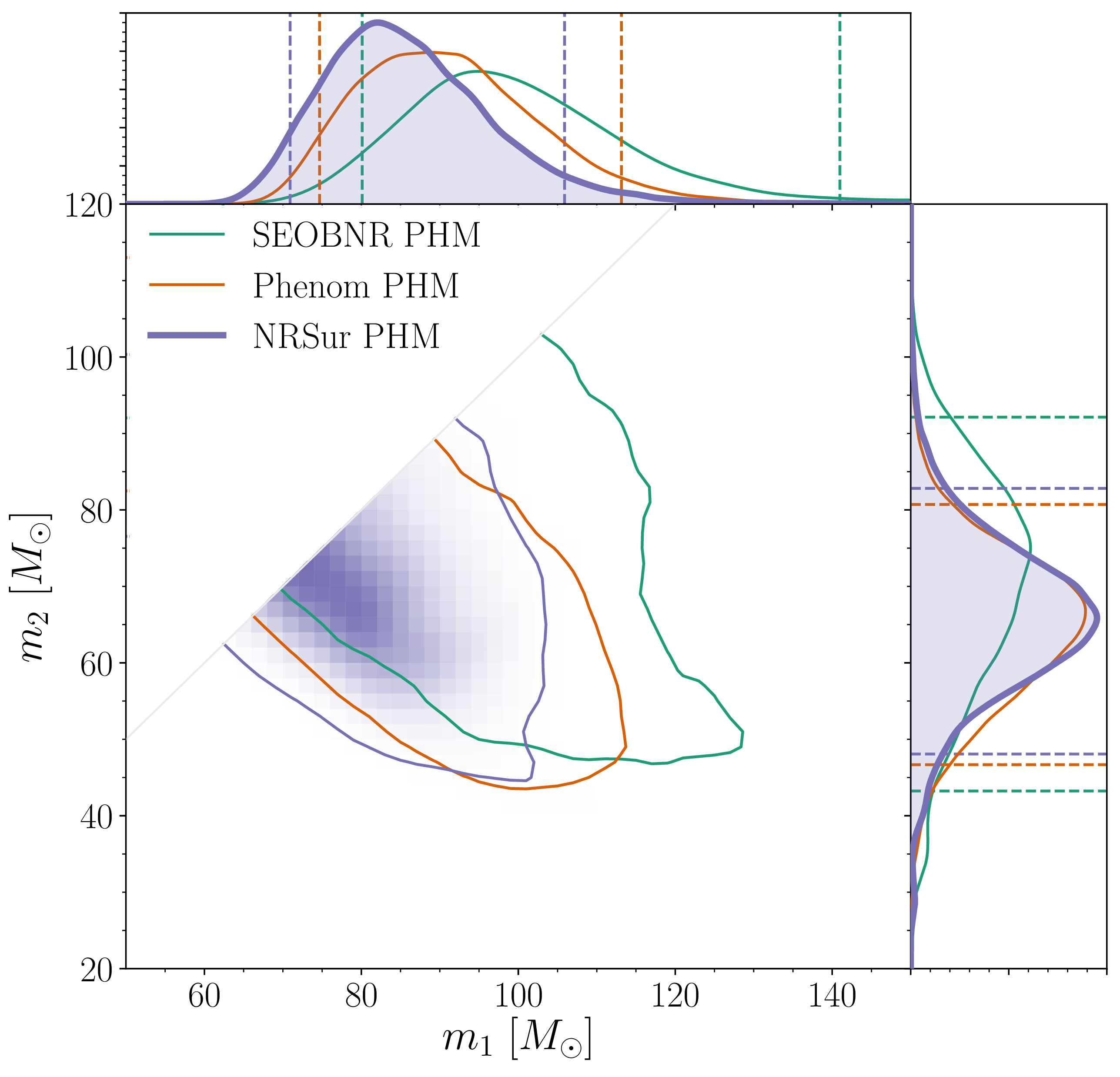
Estimated masses for the two components in the binary $m_1 \geq m_2$ . We show results several different waveform models and use the numerical relativity surrogate (NRSur PHM) as our best results. The two-dimensional shows the 90% probability contour. The dotted lines in one-dimensional plots the symmetric 90% credible interval. Part of Figure 1 of the GW190521 Implications Paper.

When you form a black hole from a star, its mass depends upon the mass of of its parent star. More massive stars generally form bigger black holes, but because of all the physics that goes on inside stars, it’s not a simple relationship. One important phenomena in determining the fate of massive stars is pair instability. When the cores of stars become very hot ( $\sim 3 \times 10^9~\mathrm{K}$ , just slightly less than the temperature of the mozerlla on that first bite of pizza, even though you should know better by now), the photons of light (gamma-rays) bouncing around inside the core become energetic enough to produce pairs of electrons and positrons [bonus note]. For the star, this causes some trouble. Its core is mostly supported by radiation pressure. If photons start disappearing as they are converted to electrons and positrons, then there isn’t as much radiation around, and the star will start to collapse. As it collapses, explosive nuclear reactions are triggered. Pair instability kicks in for stars with helium cores about $30 M_\odot$ . If the core is between $30 M_\odot$ and about $65 M_\odot$ , the star will blast off its outer layers, possibly repeating the cycle of pair-instability collapse and explosion many times. This results in smaller black holes than you might otherwise expect. For helium cores between $65 M_\odot$ and about $135 M_\odot$ , the explosion completely destroys the star, leaving nothing behind. These stars never collapse down to a black hole, and this leaves a gap, predicted to start somewhere between $45 M_\odot$ and $55 M_\odot$ .

Remnant masses for stars of different masses

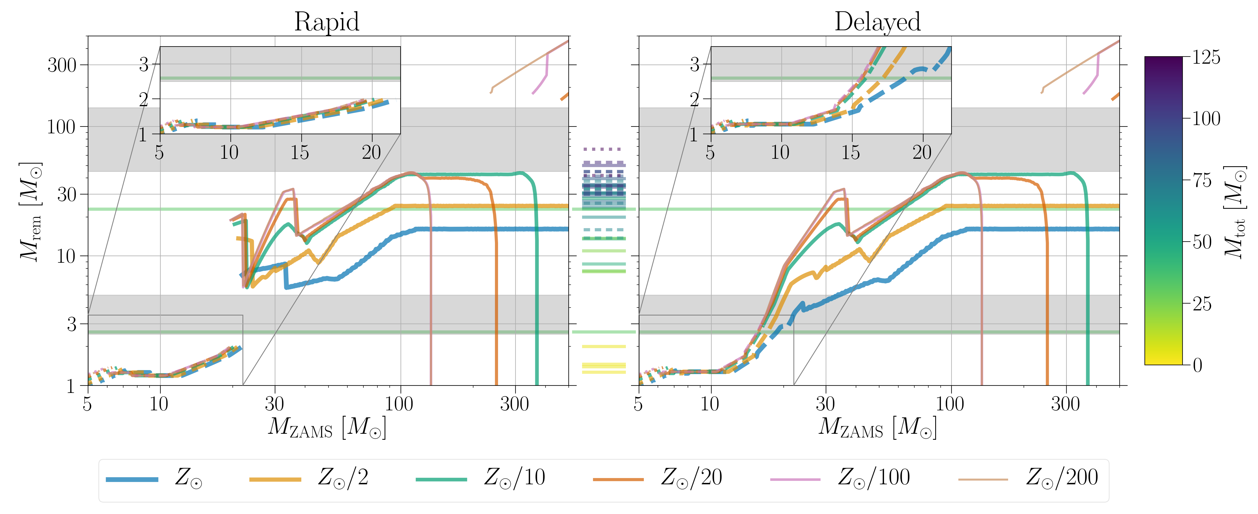
Remnant (white dwarf, neutron star or black hole) mass $M_\mathrm{rem}$ for different initial (zero age main sequence) stellar masses $M_\mathrm{ZAMS}$ . This is just for single stars, and ignores all the complicated things that can happen in binaries. The different coloured lines indicate different metallicities $Z$ (higher metallicity stars lose more mass through stellar winds). The two panels are for two different supernova models. The grey bars indicate potential mass gaps: the lower core collapse mass gap (only predicted by the Rapid model) and the upper pair-instability mass gap. The tick marks in the middle are various claimed gravitational-wave source, colour-coded by the total mass of the binary $M_\mathrm{tot}$ . Figure 1 of Zevin et al. (2020).

The more massive of GW190521’s black holes sits squarely in the expected pair-instability mass gap. How can we form such a system?

To delve into all the details, we have put together two papers on GW190521. The high mass of the system poses challenges not just for our understanding of astrophysics, but also for our data analysis. Below, I’ll go through what we have discovered.

The signal

GW190521 was first identified in our online searches about 20 seconds after we took the data. All three of our detectors were online and observing at the time. It was a short bleep of a signal indicating a high mass system. Short signals always make me suspicious as they can easily confused with some types of glitch. The signal was picked up by multiple search algorithms, which generally is a good sign, as they all estimate the background of noise in a slightly different way. However, the estimated false alarm rates were only one per few years. That’s not terribly impressive—it’s the range where things can change as we collect more data. Immediately, checks of the signal began. We have many ways of monitoring our detectors, and experts started running through these. Microphones at Hanford picked up a helicopter overhead a few minutes later, but that’s too far away in time to be related to the signal. The initial checks all looked OK, so we were confident that it was safe to share the candidate detection S190521g.

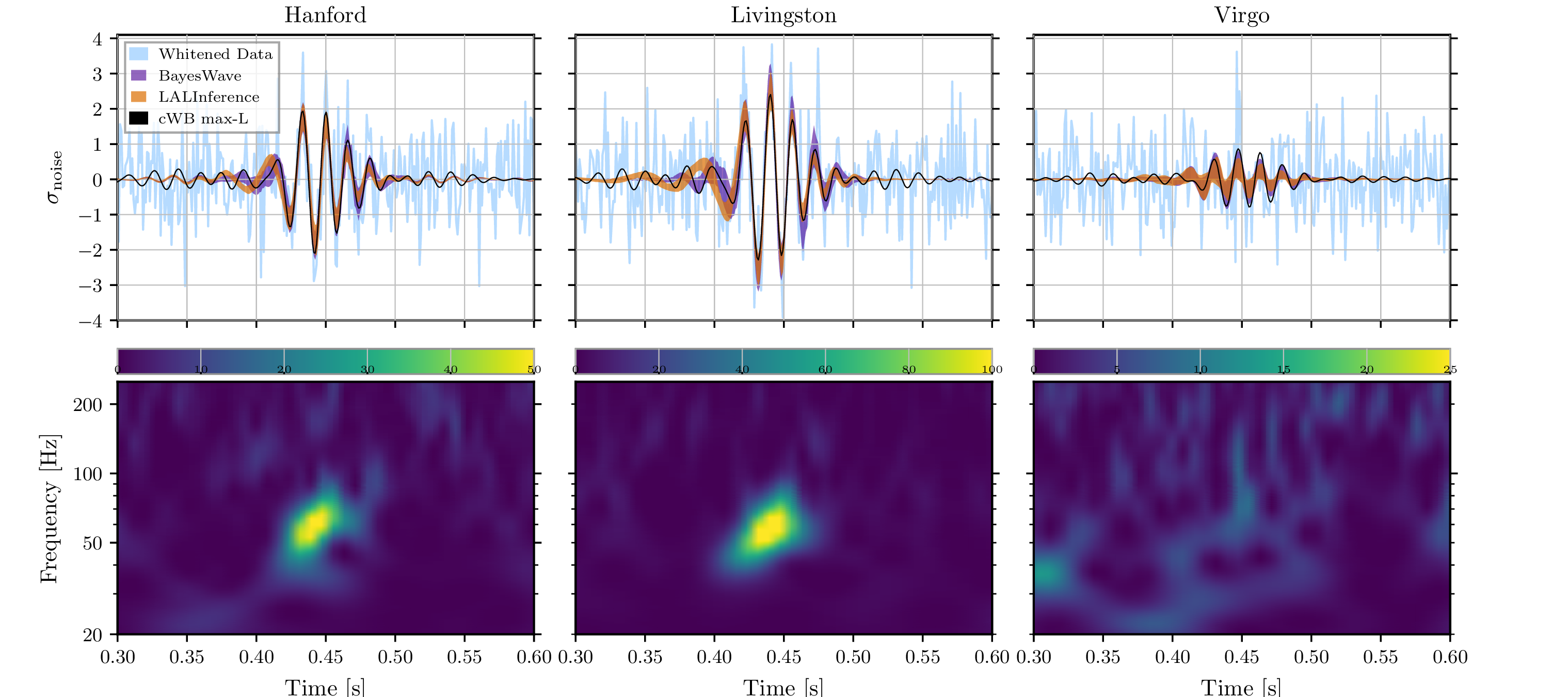
Visualisations of GW190521. The top panels show whitened data and reconstructed waveforms from the template-free detection algorithm cWB, BayesWave (which reconstructs the signal from sine–Gaussian wavelets), and our parameter estimation code LALInference (which uses binary black hole waveforms). The bottom panels show time–frequency plots: each plot has a different scale as the signal is loudest in LIGO Livingston and hardly noticeable in Virgo. As the signal is so short, we don’t see the usual chirp of a binary coalescence clearly. Figure 1 of the GW190521 Discovery Paper.

After hearing that the initial checks were complete, I went to bed, little knowing the significance of what we had found. The initial estimates for the masses of a binary come from our search pipelines—specifically the pipelines that match signal templates to the data. At high masses, the search template bank doesn’t have many templates, so the best fitting template can be quite a way from the true value. It was only after completing a proper parameter estimation analysis that we get a good idea of the masses and their uncertainties. When these results came in we found that we potentially had something lying smack in the middle of the pair-instability mass gap. That was, if the signal were real.

While initial checks of the signal showed nothing suspicious, we always do more offline checks. For GW190521 there were a few questions that took some digging to understand.

First, the peak of the signal is around 60 Hz. This is also the mains frequency in the US, so there was concern that the signal was contaminated by noise caused by this (which would obviously be shocking). A variety of careful investigations were done subtracting out noise from the mains. In the end, it turns out that this makes negligible difference to the results, which is nice.

Second, there was concern over the shape of the signal. Our template-based search algorithms always look at how well the signal matches the template: if you get a really good match in one frequency range, but not another, then that’s an indicator that you have some random noise rather than a true signal. This consistency test is summarised in a statistic, which should be around 1 if all is OK, and larger if things don’t fit. For the PyCBC algorithm, the value for the Livingston data was about 3. Since the signal was loudest in Livingston, was this cause for alarm? One explanation could be that the template wasn’t a good fit because the templates used by the search don’t include the effects of spin precession. Hence, if you have a signal where spin precession is important, you would expect a bad fit. Checking the consistency with templates which included precession did give better consistency. However, the GstLAL algorithm also used templates without precession, and its consistency test looked fine. Therefore, it couldn’t just be precession. It seems that the key is that there are so few templates in the relevant area for PyCBC’s template bank (GstLAL had things better covered). Hence, it is hard to find a good fitting template. Adding the best fitting template from the GstLAL bank to the PyCBC search leads to it being picked out as the best template too, with a consistency check statistic of 1.7 (not perfect, but not suspicious). I think this highlights the importance of not limiting yourself to only finding what you expect: we need to include the potential for our searches to discover things outside of what we have discovered in the past.

Finally, there was the difference in significance reported by the different search algorithms. In addition to the template-based searches, we also have searches which look for more generic signals without templates [bonus note], instead using the consistency in the data from different detectors to spot signals. Famously, our non-template algorithm coherent WaveBurst (cWB) made the first detection of GW150914 (other algorithms weren’t up-and-running at the time). Usually, the template searches should do better as they know what they are looking for. This has mostly been the case so far. The exception was GW170729, our previously most massive and lowest significance detection. Generally, you expect searches to disagree more on quiet signals (not too much of an issue for GW190521), as then how they characterise the noise background is more important. We also expect the template searches to lose their advantage for very short signals, when there’s not much for a template to match, and when the coherence check used by cWB comes in especially handy. GW190521 is again found with greatest significance by cWB. In our final searches (using all the data from the first six months of the third observing run), cWB gives a false alarm rate of 1 per 4900 years (pretty darn good—at least a Jammie Wagon Wheel in biscuit terms), GstLAL gives 1 per 829 years (nice—a couple of Fruit Creme biscuits), and PyCBC gives 1 per 0.94 years (not at all exciting—an Iced Gem at best). Should we be suspicious of the difference? Perhaps cWB can pick up on something extra in the signal because actually the source isn’t a quasicircular binary [bonus note] as assumed by our templates? We know that the search templates are missing some features, like the effects of spin precession, and also higher order multipole moments. Seeing how our search algorithms cope finding simulated signals that include these extra bits of physics, we find that similar discrepancies between cWB and GstLAL happen around 8% of the time, while for cWB and PyCBC they happen about 3% of the time. That’s enough to make me go Hmm, but not enough to convince me that we’ve detected a completely new type of signal, one which doesn’t come from a quasicircular binary.

The conclusion from our analysis is that GW190521 is a good-looking gravitational wave signal. We are confident that it is a real detection, even though it is really short. However, we can’t be positive that the source is quasicircular binary. That’s the most likely explanation, and consistent with what we’ve seen, but potentially not the only explanation.

There are other sources for gravitational waves beyond quasicircular binaries. One of the best known would be a supernova explosion. GW190521 is certainly not one of these. For one thing, the signals are much longer and more complicated, and for another, we could really only detect a supernova within our own galaxy, and we probably would have noticed that happen. Another hypothesised search which could produce a nice, short bleep of a signal would be a cosmic string. Vibrations or ripples along a cosmic string can source gravitational waves, and while we don’t know if cosmic strings exist, we do have templates for what these signals should look like. Using these, we can compare how well the data are described by cosmic string signals compared to our quasiciruclar binary templates. We find Bayes factors of about $10^{30}$ in favour of the binary signals, so it’s probably not cosmic strings. Finally, you’ve perhaps noticed that I’ve been writing quasicircular [bonus note] a lot. Part of that is because it’s a cool word (25 points in Scrabble), but also because it’s possible that we have an eccentric binary. These are difficult to model, so we don’t have lots of good templates for them, but when you have a short signal, it is possible that eccentricity could be confused with spin precession. This would lead us to overestimating the distance and underestimating the masses. Initial studies do seem to show that an eccentric signal fits the data well (Romero-Shaw et al. 2020; Gayathri et al. 2020). An eccentric binary is the most probable alternative to a quasicircular binary, but it is pretty improbable. Since eccentricity is lost during inspiral, we would need something to have pumped the eccentricity, which is difficult for a binary so close to merger. I would bet my Oreos on the source being a quasicircular binary.

The source properties

If we stick with the assumption of a quasicircular binary, what can we tell about the source? We have already covered the component masses of $m_1 = 85^{+21}_{-14} M_\odot$ and $m_2 = 66^{+17}_{-18} M_\odot$ , and that the merger remnant is $M_\mathrm{f} = 142^{+28}_{-16} M_\odot$ . The plot below shows the final mass as well as the spin, which is $\chi_\mathrm{f} = 0.72^{+0.09}_{-0.12}$ . For the black holes formed from the mergers of near equal mass binaries, you’d expect the final spin to be around $0.7$ .

Estimated mass $M_\mathrm{f}$ and spin $\chi_\mathrm{f}$ for the final black hole. We show results several different waveform models and use the numerical relativity surrogate (NRSur PHM) as our best results. The two-dimensional shows the 90% probability contour. The dotted lines in one-dimensional plots the symmetric 90% credible interval. The mass is safely above the conventional lower limit to be considered an intermediate-mass black hole. Figure 3 of the GW190521 Implications Paper.

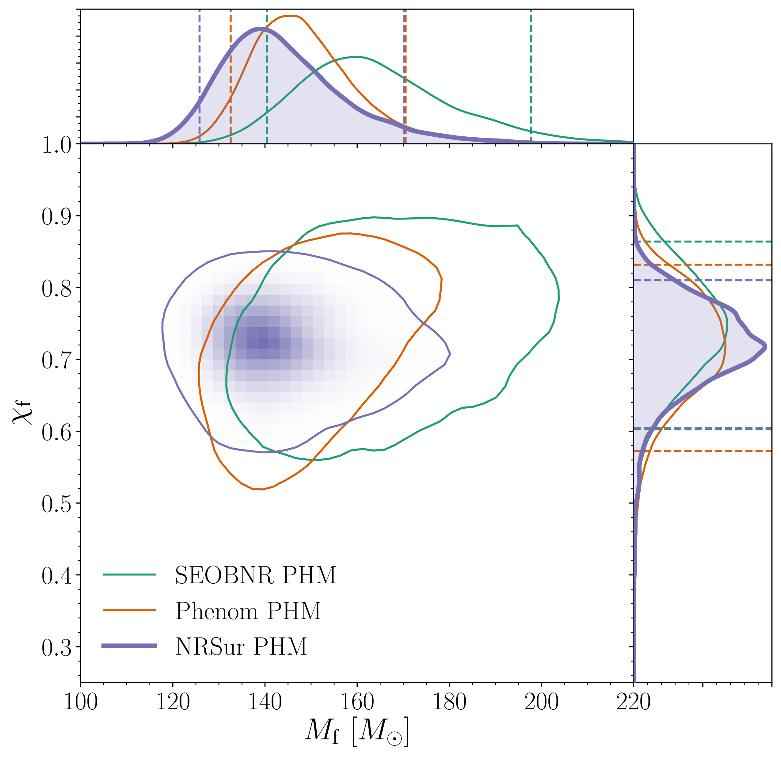
We can also get an estimate of the final spin from the final part of the signal, the ringdown. This is where the black hole settles down to its final state, like me after 6 pm. What is neat about using the ringdown is that we don’t need to assume that the binary was quasicircular, as we only care about the black hole formed at the end. The downside is that we don’t get an estimate of the distance, so we only measure the redshifted final mass $(1+z)M_\mathrm{f}$ . Looking at the ringdown, we get lovely consistent results trying ringdown models at different start times and including different higher order multipole moments, and all agree with the analysis of the entire signal using the quasicircular templates.

Final black hole mass and spin measured from GW190521's ringdown

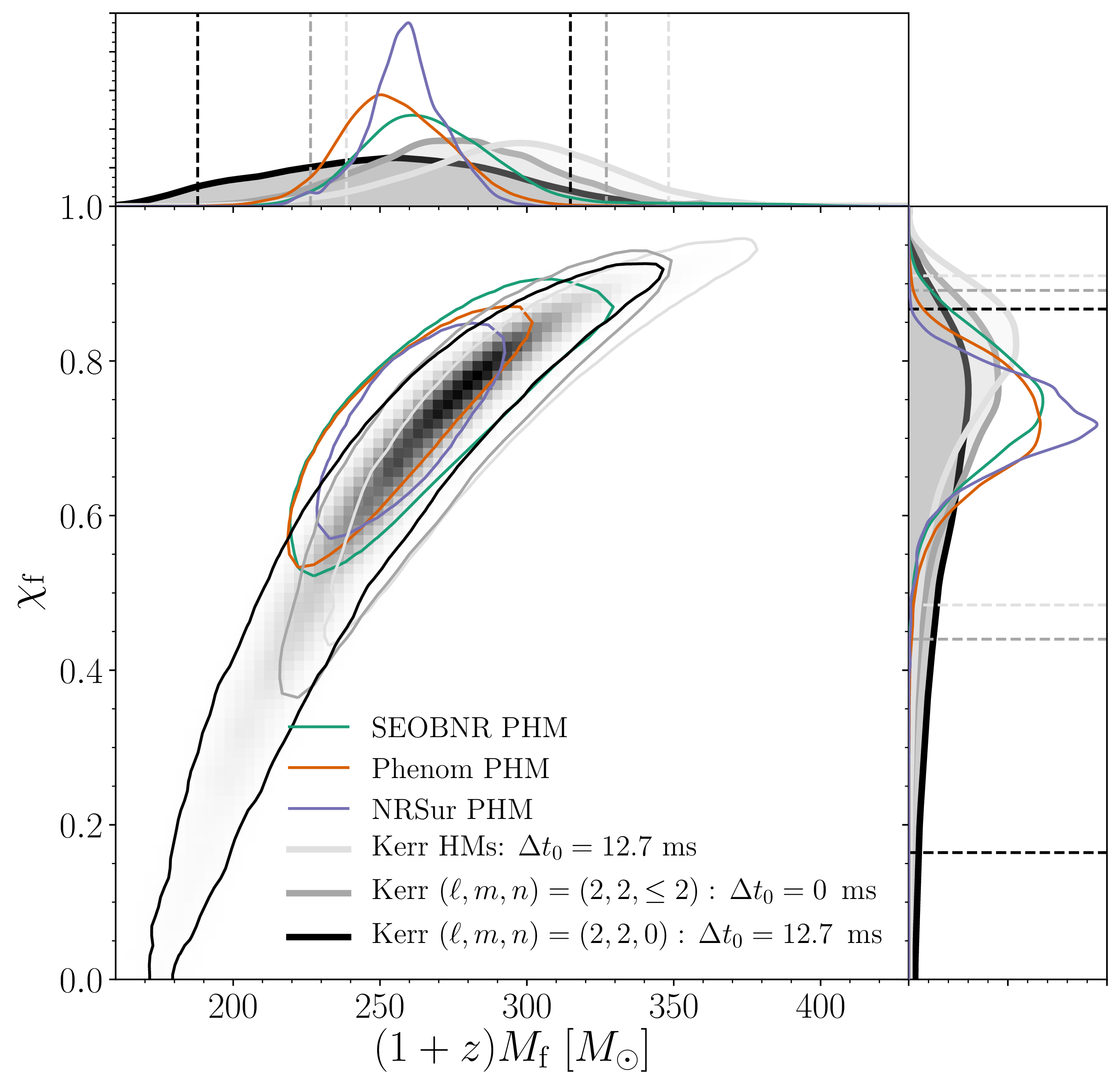
Estimated redshifted mass $(1+z)M_\mathrm{f}$ and spin $\chi_\mathrm{f}$ for the final black hole. We show results several different insprial–merger–ringdown waveform models, which we use for our standard analysis, as well as ringdown-only waveforms. They agree nicely. The two-dimensional shows the 90% probability contour. The dotted lines in one-dimensional plots the symmetric 90% credible interval. The mass is safely above the conventional lower limit to be considered an intermediate-mass black hole. Part of Figure 9 of the GW190521 Implications Paper.

Being able to measure the ringdown at all is an achievement. It’s only possible for loud signals from high mass systems. The consistency of the mass and spin estimates is not only a check of the quasicircular analysis. It is much more powerful than that. The ringdown measurements are a test of the black hole nature of the final object. All looks as expected so far. I really want to do this for louder signals in the future.

Returning to the initial binary, what can we say about the spins of the initial black holes? Not much, as it is difficult to extract information from such a short waveform.

The spin components aligned with the orbital angular momentum affect the transition from inspiral, and have a small influence on the final spin. We often quantify the aligned components of the spin in the mass-weighted effective inspiral spin parameter $\chi_\mathrm{eff}$ , which goes from $-1$ for both the spins being maximal and antialigned with the orbital angular momentum to $1$ for both spins being maximal and aligned with the orbital angular momentum. We find that $\chi_\mathrm{eff} = 0.08^{+0.27}_{-0.36}$ , consistent with no spin, spins antialigned with each other or in the orbital plane. The result is strongly influenced by the assumed prior, we’ve not learnt much from the signal.

The component of the spin in the orbital plane (perpendicular to the orbital angular momentum) control the amount of spin precession. We often quantify this using the effective precession spin parameter $\chi_\mathrm{p}$ , which goes from $0$ for no in-plane spin, to $1$ for maximal precession. Precession normally shows up in the modulation of the inspiral signal, so you wouldn’t expect to measure it well from a short signal. However, it can also influence to amplitude of the signal around merger, and we seem to get a bit of information here, which seems to prefer larger $\chi_\mathrm{p}$ . We find $\chi_\mathrm{p} = 0.68^{+0.28}_{-0.34}$ , but there’s support across the entire range.

Effective inspiral spin and effective precession spin for GW190521

Estimated effective inspiral spin $\chi_\mathrm{eff}$ and effective precession spin $\chi_\mathrm{p}$ . We show results several different waveform models and use the numerical relativity surrogate (NRSur PHM) as our best results. The two-dimensional shows the 90% probability contour. The dotted lines in one-dimensional plots the symmetric 90% credible interval. We also show the prior distributions in the one-dimensional plots. Part of Figure 1 of the GW190521 Implications Paper.

Looking at the spins overall, the lack of aligned spin plus the support for in-plane spins means that we prefer misaligned spins. You wouldn’t expect this for two stars which have lived their lives together as a binary, but it wouldn’t be implausible for a dynamically formed binary. A dynamical formation seems plausible to me, but since the spin measurements aren’t too concrete, we can’t really rule too much out [bonus note].

Finally, let’s take a look at the distance to the source. Our analysis gives a luminosity distance of $D_\mathrm{L} 5.3^{+2.4}_{-2.6}~\mathrm{Gpc}$ . This makes the source a good contender for the most distant gravitational wave source ever found [bonus note]. It’s actually far enough, that we might want to reconsider our standard approximation that sources are uniformly distributed like $D_\mathrm{L}^2$ . This would be OK if sources were uniformly distributed in a non-evolving Universe, but sadly we don’t live in such a thing, and we have to take into account the expansion of the Universe, and the evolution of the galaxies and stars within it. We’ll come back to look at this when we present our catalogue of detections from the first part of the third observing run.

The astrophysics

Exploring the upper mass gap

The location of the upper mass gap is pretty well determined. There are a variety of uncertainties in the input physics, such as the nuclear reaction rate for burning carbon into oxygen, the treatment of convection inside stars or if stars rapidly rotate which can alter the cut-off. No-one has tried varying all these together, but individually you can’t get above about $55 M_\odot$ for your black hole. Allowing for new types of particles (like axions, one of the candidates for dark matter, and possibly the explanation for why teenage boys can smell terrible) can potentially increase the limit to above $70 M_\odot$ , but that is extremely speculative (I’d love it if it were true). Sticking to known physics, at face value, it is hard to explain the mass of the primary black hole from our understanding of how stars evolve.

There are potentially ways around the mass gap with help from a star’s environment:

Super efficient accretion from a companion star can grow black holes into the mass gap. Then you wouldn’t expect the total mass of the binary to over about $100 M_\odot$ , so we’d need to swap out partners in this case.
The pair instability originates in the helium core of a star. If we can find a way to grow the envelope of the star, while keeping the core below the threshold for the instability to set in, then the whole thing could collapse down to a mass gap black hole. This could potentially happen if two stars collide after one has already formed its helium core. The other gets disrupted and swells the envelope. This might be expected in stellar clusters. Similarly, a couple of recent papers (Farrell et al. 2020; Kinugawa, Nakamura & Nakano 2020) have also suggested that the first generation of stars, which have few elements other than hydrogen or helium, could also collapse down to black holes in this mass range. The idea here is that these stars lose much less of their envelopes due to stellar winds, so you can end up with what we would otherwise consider an oversized envelope around a core below the pair instability threshold
We could have two black holes merge to form a bigger one, and then have the remnant go on to form a new binary. You would need a dense environment for this, somewhere like a globular cluster where it’s easy to find new partners. Ideally, somewhere with a large escape velocity, perhaps a nuclear star cluster, which has a high escape velocity so that it is more difficult for the remnant black hole to get kicked out at any point: gravitational waves give a recoil kick, and close encounters with other objects can also lead to the initial binary getting a kick.
Especially good for growing black holes may be if they are embedded in the accretion disc around a supermassive black hole. Then these disc black holes can merge with each other whilst being unlikely to escape the environment. Additionally, they can swallow lots of gas from the surrounding disc to help them grow big and strong.

There is also the potential that we don’t have a black hole formed from stellar collapse, but instead a primordial black hole formed from dense regions in the early Universe. These primordial black holes are a another candidate for dark matter. I like that there are two options for potential dark matter-related formation channels. It’s good to have options.

The difficulty with all of these alternative formation channels is matching the observed rate for GW190521-like systems. It’s not enough for a proposed channel to be able to explain the system’s properties, it also needs to make enough of them for us to have come across one. From our data, we infer that GW190521-like systems have a merger rate density of $0.13^{+0.30}_{-0.11}~\mathrm{Gpc^{-3}\,yr^{-1}}$ . Predicted rates for the various formation mechanisms discussed above can be rather uncertain (kind of like how the exact value of a small bag full of Bitcoin is uncertain), so I would like to see more work on this, before picking a most plausible option.

Hierarchical mergers

We did do some quantitative analysis for the case of hierarchical mergers of black holes, following the framework outlined in Kimball et al. (2020). This simultaneously fits the mass and spin distribution for the first generation (1g) of black holes formed from stars, and a fraction of hierarchical mergers involving second generation (2g) merger remnants. To calibrate the number of hierarchical mergers, we use globular cluster simulations.

Using our base model, where the 1g+1g population is basically the Model C we used to describe our detections from the first two observing runs, we find that the odds are in favour of GW190521 being a 1g+1g merger. Hierarchical mergers are so rare, that it’s actually more probable that we squish down the inferred masses and have something from the tail of the 1g population.

The rate of hierarchical mergers, however, is very sensitive to the distribution of spins of 1g black holes. Larger spins give bigger kicks (even a spin of 0.1 is enough to mean remnants are hardly ever retained in typical globular clusters). If we add into the mix a fraction of 1g+1g binaries which have 0 spin (motivated by recent simulations), we improve the odds to be roughly even 1g+1g vs 1g+2g, and less common for 2g+2g. Given that we are not taken into account that only a fraction of binaries would be in clusters, which would reduce the odds of a hierarchical merger considerably, this isn’t quite enough to convince me.

However, what if we were to turn up the mass of the cluster? For our globular cluster model, we used $5\times 10^5 M_\odot$ , what if we tried $10^8 M_\odot$ , more like you would expect for a nuclear star cluster? We shouldn’t really be doing this, as our model is calibrated against globular cluster simulations, and nuclear star clusters have different dynamics, but we can use our results as illustrative. In this case, we find odds of about 1000:1 in favour of hierarchical mergers. This suggests that this option may be a promising one to follow, but we must moderate our results remembering that only a fraction of binaries would form in these dense environments.

The analysis is done using only our first 10 detected binary black hole from our first two observing runs plus GW190521. GW190521 is not the most representative of the third observing run detections (hence why it gets special papers™), so it is not exactly fair to stick it in to the mix to infer the population parameters. We’ll need to redo this analysis when we have the full results of the run to update the results. Having more binaries in the analysis should allow us to more precisely measure the population parameters, so we will be more confident in our results.

The surprise

After all our investigations, we thought we had examined every aspect of GW190521. However, there’s always one more thing. As we were finishing up the paper, a potential electromagnetic counterpart was announced.

Electromagnetic counterparts are not expected when two black holes merge—black holes are indeed black—however, material around the binary could produce light.

The counterpart was found by the Zwicky Transient Factory. They targeted active galactic nuclei to look for counterparts. These are the bright cores of galaxies where the supermassive black hole is feeding off a surrounding disc. In this case, they hypothesis that the binary had some gas orbiting around it, and when the binary merged, the gravitational wave recoil kick sent the remnant black hole and its orbiting material into the disc of the supermassive black hole. As the orbiting material crashes into the disc it will emit light. Then, once it is blasted away, material from the disc accreting onto the remnant black hole will also emit light. This seems to fit with what was observed, with the later powering the observed emission.

What I think is exciting about this proposal is that active galactic nuclei are one of the channels predicted to produce binaries as massive as GW190521! Therefore, things seem to line up nicely.

Three dimensional localisation and active galactic nucleus location

The three dimensional localisation for GW190521. The lines indicate the position of the claimed electromagnetic counterpart from around an active galactic nucleus. This location lies at the 70% credible level. Credit: Will Farr

What I think is less certain is if the counterpart is really associated with our gravitational wave source. The observing team estimate that the probability of a chance association is small. However, there is a lot of uncertainty in how active galactic nuclei can flare. The good news is that the remnant black hole may continue to orbit and hit the disc again, leading to another flare. The bad news is that the uncertainty on when this happens is many years, so we don’t know when to look.

Follow-up analyses by Ashton et al. (2020) and Palmese et al. (2021) cast the association as more uncertain. It is difficult to be confident of an association when the localization volume is so large. If we knew that this type of flare had to look exactly like the observed emission, that would help, but we can’t be that certain yet.

Overall, I think we need to observe another similar association before we can be certain what’s going on. I really hope this candidate counterpart encourages people to follow up more binary black holes to look for emission. The unexpected discoveries are often the most rewarding.

The papers

The GW190521 Discovery Paper

Title: GW190521: A binary black hole merger with a total mass of 150 solar masses
Journal: Physical Review Letters; 125(10):101102(17)
arXiv: 2009.01075 [gr-qc]
Read this if: You want to understand the detection of GW190521

This is the paper announcing the gravitational wave detection. It follows our now standard pattern for a detection paper of discussing our instruments and data quality; our detection algorithms and the statistical significance of the search; the inferred properties of the source, and a bit of testing gravity; a check of the reconstruction of the waveform, and then a nice summary looking forward to more discoveries to come.

What is a little different for this paper is that because the signal is so short, we have had to be extra careful in our checks of the detectors’ statuses, the reliability of our detection algorithms, and the assumptions that go into estimating the source properties. If you are sceptical of being able to detect such short signals, I recommend checking out the Supplemental Material for a summary of some of the tests we did.

The GW190521 Implications Paper

Title: Properties and astrophysical implications of the 150 solar mass binary black hole merger GW190521
Journal: Astrophysical Journal Letters; 900(1):L13(27)
arXiv: 2009.01190 [astro-ph.HE]
Read this if: You want to understand the implications for fundamental physics and astrophysics of the discovery

In this paper we explore the properties of GW190521. We check the robustness of the inferred source properties. For such a short signal, our usual assumption that we have a quasicircular binary is probably the most sensible thing to do, but we can’t be certain, and if this assumption is wrong, then we will have got the properties wrong. Astronomy is hard sometimes. Assuming that our estimates of the properties are correct, we look at potential formation mechanisms. We don’t come to any firm conclusions, but sketch out some of the possibilities. We also look at tests of the black hole nature of the final object in a bit more detail. A few wibbles can sure cause a lot of excitement.

Science summary: GW190521: The most massive black hole collision observed to date
Data release: Gravitational Wave Open Science Center; Parameter estimation results
Rating: 🍰🐋📏🏆

Bonus notes

Squeezing

Please hug responsibly.

Minimum black hole mass

The uncertainty in when gravity will take over and squish things down to a black hole is set by the stiffness of neutron star matter. Neutron stars are the densest matter can be, this is the stiffest form of matter, the one most resistant to being crushed down into a black hole. The amount of weight neutron star matter can support is uncertain, so we don’t quite know their maximum mass yet. This made the discovery of GW190814 particularly intriguing. This gravitational wave came from a binary where the less massive component was about $2.6 M_\odot$ , exactly in the range where we’d expect the transition between neutron stars and black holes. We can’t tell for certain which it is, but I’ve bet my M&Ms on a black hole.

It’s potentially possible that there are black holes smaller than the maximum neutron star mass which didn’t form from collapsing stars. These are primordial black holes, which formed from overdense regions in the early universe. We don’t know for certain if they do exist, but we are looking.

Positrons

Positrons are antielectrons, the antimatter equivalent of electrons. This means that they share identical properties to electrons except that they have opposite charge. Electrons things that the glass is half-empty, positrons think it is half-full. Neutrinos think that the glass is twice as big as it needs to be, but so long as we have a well-mixed cocktail, who cares?

Burst searches

In the jargon of LIGO and Virgo, we refer to the non-template detection algorithms as Burst searches, as they are good at spotting bursts of gravitational waves. Burst is not a terribly useful description if you’ve not met it before, so we generally try to avoid this in our papers. A common description is an unmodelled search, to distinguish from the template-based searches which use model waveforms as input. However, it’s not really true that the Burst searches don’t make modelling assumptions about the signal. For example, the cWB algorithm used to look for binaries assumes that the frequency will increase with time (as you would expect for an inspiralling binary). To avoid this, we’ve sometimes describes the search algorithm as weakly modelled, but that’s perhaps no clearer than Burst. For this post, I’ll stick to non-template as a description.

Quasicircular

When talking about the orbits of binaries, we might be interested in their eccentricity. Eccentricity is a key tracer of how the binary formed. As binaries emit gravitational waves, they quickly lose their eccentricity, so in general we don’t expect there to be significant eccentricity for the binaries detected by LIGO and Virgo.

An orbit with zero eccentricity should be circular. However, since we have a binary emitting gravitational waves the orbit will be shrinking. As we have an inspiral, if you were to trace out the orbit, it would not be a circle, even though we would describe it as having zero eccentricity. This is particularly noticeable at the end of the inspiral, when we get close to the two objects plunging together. Hence, we describe orbits as quasicircular, which I think sounds rather cute.

The simulation above shows the orbit of an inspiral. Here the spins of the black holes also lead to the precession of the orbit, making it a bit more complicated than you might expect for a something described as circular, but, of course, not at all unexpected for something with a cool name like quasicircular. I also really like how this visualisation shows the event horizons of the two black holes merging.

Spin Bayes factors

To try to quantify the support for spin, we quote two Bayes factors. The first is for spin verses no spin. There we find a Bayes factor of about 8.3 in favour of there being spin. That’s not something you’d want to bet against, but for comparison, for GW190412 we found that is it over 400, and for GW151226 it is over a million. I’d expect any statement on spins for GW190521 will depend upon your prior assumptions. The second Bayes factor is in favour of measurable precession. This is not the same as comparing the Bayes factor between perfectly aligned spins (when there would be no precession) and generic, isotropically distributed spins. Instead we are comparing the scenario where we can measure in-plane spins verses the case where there are isotropically distributed but the in-plane spins don’t have any discernible consequences. Here we find a Bayes factor of 11.5 in favour of measurable precession. This makes sense as we do have some information on $\chi_\mathrm{p}$ , and would expect an even Bayes factor of 1 if we only got the prior back. It seems we have gained some information about the spins from the signal.

For more on Bayes factors, I would suggest reading Zevin et al. (2020). In particular, this explains why it can make sense here that the Bayes factor for measurable precession is larger than the Bayes factor for there being spin. At first, it might appear odd that we can be more definite that there is precession than any spin at all. However, this is because in comparing spin verses no spin we are hit by the Occam factor—we are adding extra parameters to our model, and we are penalised for this. If the effects of spins are small, so that they are not worth including, we would expect no-spin to win. When looking at the measurability of precession, we have set up the comparison so that there is no Occam factor. We can only win, if waveforms with precession clearly fit the data better, or break even if they make no difference.

Economically large

To put a luminosity distance of $5.3~\mathrm{Gpc}$ in context, if you put $1 in a jar ever two weeks over the duration the gravitational wave signal was travelling from its source to us (7.1 billion years, about 1.5 times the age of the Sun), you would end up with about a net worth only 7% less than Jeff Bezos (currently $199.3 billion).

Observing run 1—The papers

September 24, 2017October 13, 2017 / CPLB / Leave a comment

The second observing run (O2) of the advanced gravitational wave detectors is now over, which has reminded me how dreadfully behind I am in writing about papers. In this post I’ll summarise results from our first observing run (O1), which ran from September 2015 to January 2016.

I’ll add to this post as I get time, and as papers are published. I’ve started off with papers searching for compact binary coalescences (as these are closest to my own research). There are separate posts on our detections GW150914 (and its follow-up papers: set I, set II) and GW151226 (this post includes our end-of-run summary of the search for binary black holes, including details of LVT151012).

Transient searches

The O1 Binary Neutron Star/Neutron Star–Black Hole Paper

Title: Upper limits on the rates of binary neutron star and neutron-star–black-hole mergers from Advanced LIGO’s first observing run
arXiv: 1607.07456 [astro-ph.HE]
Journal: Astrophysical Journal Letters; 832(2):L21(15); 2016

Our main search for compact binary coalescences targets binary black holes (binaries of two black holes), binary neutron stars (two neutron stars) and neutron-star–black-hole binaries (one of each). Having announced the results of our search for binary black holes, this paper gives the detail of the rest. Since we didn’t make any detections, we set some new, stricter upper limits on their merger rates. For binary neutron stars, this is $12,600~\mathrm{Gpc}^{-3}\,\mathrm{yr}^{-1}$ .

More details: O1 Binary Neutron Star/Neutron Star–Black Hole Paper Paper summary

The O1 Gamma-Ray Burst Paper

Title: Search for gravitational waves associated with gamma-ray bursts during the first Advanced LIGO observing run and implications for the origin of GRB 150906B
arXiv: 1611.07947 [astro-ph.HE]
Journal: Astrophysical Journal; 841(2):89(18); 2016
LIGO science summary: What’s behind the mysterious gamma-ray bursts? LIGO’s search for clues to their origins

Some binary neutron star or neutron-star–black-hole mergers may be accompanied by a gamma-ray burst. This paper describes our search for signals coinciding with observations of gamma-ray bursts (including GRB 150906B, which was potentially especially close by). Knowing when to look makes it easy to distinguish a signal from noise. We don’t find anything, so we we can exclude any close binary mergers as sources of these gamma-ray bursts.

More details: O1 Gamma-Ray Burst Paper summary

The O1 Intermediate Mass Black Hole Binary Paper

Title: Search for intermediate mass black hole binaries in the first observing run of Advanced LIGO
arXiv: 1704.04628 [gr-qc]
Journal: Physical Review D; 96(2):022001(14); 2017
LIGO science summary: Search for mergers of intermediate-mass black holes

Our main search for binary black holes in O1 targeted systems with masses less than about 100 solar masses. There could be more massive black holes out there. Our detectors are sensitive to signals from binaries up to a few hundred solar masses, but these are difficult to detect because they are so short. This paper describes our specially designed such systems. This combines techniques which use waveform templates and those which look for unmodelled transients (bursts). Since we don’t find anything, we set some new upper limits on merger rates.

More details: O1 Intermediate Mass Black Hole Binary Paper summary

The O1 Burst Paper

Title: All-sky search for short gravitational-wave bursts in the first Advanced LIGO run
arXiv: 1611.02972 [gr-qc]
Journal: Physical Review D; 95(4):042003(14); 2017

If we only search for signals for which we have models, we’ll never discover something new. Unmodelled (burst) searches are more flexible and don’t assume a particular form for the signal. This paper describes our search for short bursts. We successfully find GW150914, as it is short and loud, and burst searches are good for these type of signals, but don’t find anything else. (It’s not too surprising GW151226 and LVT151012 are below the threshold for detection because they are longer and quieter than GW150914).

More details: O1 Burst Paper summary

The O1 Binary Neutron Star/Neutron Star–Black Hole Paper

Synopsis: O1 Binary Neutron Star/Neutron Star–Black Hole Paper
Read this if: You want a change from black holes
Favourite part: We’re getting closer to detection (and it’ll still be interesting if we don’t find anything)

The Compact Binary Coalescence (CBC) group target gravitational waves from three different flavours of binary in our main search: binary neutron stars, neutron star–black hole binaries and binary black holes. Before O1, I would have put my money on us detecting a binary neutron star first, around-about O3. Reality had other ideas, and we discovered binary black holes. Those results were reported in the O1 Binary Black Hole Paper; this paper goes into our results for the others (which we didn’t detect).

To search for signals from compact binaries, we use a bank of gravitational wave signals to match against the data. This bank goes up to total masses of 100 solar masses. We split the bank up, so that objects below 2 solar masses are considered neutron stars. This doesn’t make too much difference to the waveforms we use to search (neutrons stars, being made of stuff, can be tidally deformed by their companion, which adds some extra features to the waveform, but we don’t include these in the search). However, we do limit the spins for neutron stars to less the 0.05, as this encloses the range of spins estimated for neutron star binaries from binary pulsars. This choice shouldn’t impact our ability to detect neutron stars with moderate spins too much.

We didn’t find any interesting events: the results were consistent with there just being background noise. If you read really carefully, you might have deduced this already from the O1 Binary Black Hole Paper, as the results from the different types of binaries are completely decoupled. Since we didn’t find anything, we can set some upper limits on the merger rates for binary neutron stars and neutron star–black hole binaries.

The expected number of events found in the search is given by

$\Lambda = R \langle VT \rangle$

where $R$ is the merger rate, and $\langle VT \rangle$ is the surveyed time–volume (you expect more detections if your detectors are more sensitive, so that they can find signals from further away, or if you leave them on for longer). We can estimate $\langle VT \rangle$ by performing a set of injections and seeing how many are found/missed at a given threshold. Here, we use a false alarm rate of one per century. Given our estimate for $\langle VT \rangle$ and our observation of zero detections we can, calculate a probability distribution for $R$ using Bayes’ theorem. This requires a choice for a prior distribution of $\Lambda$ . We use a uniform prior, for consistency with what we’ve done in the past.

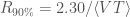
With a uniform prior, the $c$ confidence level limit on the rate is

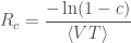
$\displaystyle R_c = \frac{-\ln(1-c)}{\langle VT \rangle}$ ,

so the 90% confidence upper limit is $R_{90\%} = 2.30/\langle VT \rangle$ . This is quite commonly used, for example we make use of it in the O1 Intermediate Mass Black Hole Binary Search. For comparison, if we had used a Jeffrey’s prior of $1/\sqrt{\Lambda}$ , the equivalent results is

$\displaystyle R_c = \frac{\left[\mathrm{erf}^{-1}(c)\right]^2}{\langle VT \rangle}$ ,

and hence $R_{90\%} = 1.35/\langle VT \rangle$ , so results would be the same to within a factor of 2, but the results with the uniform prior are more conservative.

The plot below shows upper limits for different neutron star masses, assuming that neutron spins are (uniformly distributed) between 0 and 0.05 and isotropically orientated. From our observations of binary pulsars, we have seen that most of these neutron stars have masses of ~1.35 solar masses, so we can also put a limit of the binary neutron star merger rate assuming that their masses are normally distributed with mean of 1.35 solar masses and standard deviation of 0.13 solar masses. 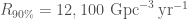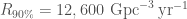This gives an upper limit of $R_{90\%} = 12,100~\mathrm{Gpc}^{-3}\,\mathrm{yr}^{-1}$ for isotropic spins up to 0.05, and $R_{90\%} = 12,600~\mathrm{Gpc}^{-3}\,\mathrm{yr}^{-1}$ if you allow the spins up to 0.4.

Upper merger rate limits for binary neutron stars

90% confidence upper limits on the binary neutron star merger rate. These rates assume randomly orientated spins up to 0.05. Results are calculated using PyCBC, one of our search algorithms; GstLAL gives similar results. Figure 4 of the O1 Binary Neutron Star/Neutron Star–Black Hole Paper.

For neutron star–black hole binaries there’s a greater variation in possible merger rates because the black holes can have a greater of masses and spins. The upper limits range from about $R_{90\%} = 1,200~\mathrm{Gpc}^{-3}\,\mathrm{yr}^{-1}$ to $3,600~\mathrm{Gpc}^{-3}\,\mathrm{yr}^{-1}$ for a 1.4 solar mass neutron star and a black hole between 30 and 5 solar masses and a range of different spins (Table II of the paper).

It’s not surprising that we didn’t see anything in O1, but what about in future runs. The plots below compare projections for our future sensitivity with various predictions for the merger rates of binary neutron stars and neutron star–black hole binaries. A few things have changed since we made these projections, for example O2 ended up being 9 months instead of 6 months, but I think we’re still somewhere in the O2 band. We’ll have to see for O3. From these, it’s clear that a detection on O1 was overly optimistic. In O2 and O3 it becomes more plausible. This means even if we don’t see anything, we’ll be still be doing some interesting astrophysics as we can start ruling out some models.

Comparison of upper limits for binary neutron star (BNS; top) and neutron star–black hole binaries (NSBH; bottom) merger rates with theoretical and observational limits. The blue bars show O1 limits, the green and orange bars show projections for future observing runs. Figures 6 and 7 from the O1 Binary Neutron Star/Neutron Star–Black Hole Paper.

Binary neutron star or neutron star–black hole mergers may be the sources of gamma-ray bursts. These are some of the most energetic explosions in the Universe, but we’re not sure where they come from (I actually find that kind of worrying). We look at this connection a bit more in the O1 Gamma-Ray Burst Paper. The theory is that during the merger, neutron star matter gets ripped apart, squeezed and heated, and as part of this we get jets blasted outwards from the swirling material. There are always jets in these type of things. We see the gamma-ray burst if we are looking down the jet: the wider the jet, the larger the fraction of gamma-ray bursts we see. By comparing our estimated merger rates, with the estimated rate of gamma-ray bursts, we can place some lower limits on the opening angle of the jet. If all gamma-ray bursts come from binary neutron stars, the opening angle needs to be bigger than $2.3_{-1.7}^{+1.7}~\mathrm{deg}$ and if they all come from neutron star–black hole mergers the angle needs to be bigger than $4.3_{-1.9}^{+3.1}~\mathrm{deg}$ .

The O1 Gamma-Ray Burst Paper

Synopsis: O1 Gamma-Ray Burst Paper
Read this if: You like explosions. But from a safe distance
Favourite part: We exclude GRB 150906B from being associated with galaxy NGC 3313

Gamma-ray bursts are extremely violent explosions. They come in two (overlapping) classes: short and long. Short gamma-ray bursts are typically shorter than ~2 seconds and have a harder spectrum (more high energy emission). We think that these may come from the coalescence of neutron star binaries. Long gamma-ray bursts are (shockingly) typically longer than ~2 seconds, and have a softer spectrum (less high energy emission). We think that these could originate from the collapse of massive stars (like a supernova explosion). The introduction of the paper contains a neat review of the physics of both these types of sources. Both types of progenitors would emit gravitational waves that could be detected if the source was close enough.

The binary mergers could be picked up by our templated search (as reported in the O1 Binary Neutron Star/Neutron Star–Black Hole Paper): we have a good models for what these signals look like, which allows us to efficiently search for them. We don’t have good models for the collapse of stars, but our unmodelled searches could pick these up. These look for the same signal in multiple detectors, but since they don’t know what they are looking for, it is harder to distinguish a signal from noise than for the templated search. Cross-referencing our usual searches with the times of gamma-ray bursts could help us boost the significance of a trigger: it might not be noteworthy as just a weak gravitational-wave (or gamma-ray) candidate, but considering them together makes it much more unlikely that a coincidence would happen by chance. The on-line RAVEN pipeline monitors for alerts to minimise the chance that miss a coincidence. As well as relying on our standard searches, we also do targeted searches following up on gamma-ray bursts, using the information from these external triggers.

We used two search algorithms:

X-Pipeline is an unmodelled search (similar to cWB) which looks for a coherent signal, consistent with the sky position of the gamma-ray burst. This was run for all the gamma-ray bursts (long and short) for which we have good data from both LIGO detectors and a good sky location.
PyGRB is a modelled search which looks for binary signals using templates. Our main binary search algorithms check for coincident signals: a signal matching the same template in both detectors with compatible times. This search looks for coherent signals, factoring the source direction. This gives extra sensitivity (~20%–25% in terms of distance). Since we know what the signal looks like, we can also use this algorithm to look for signals when only one detector is taking data. We used this algorithm on all short (or ambiguously classified) gamma-ray bursts for which we data from at least one detector.

In total we analysed times corresponding to 42 gamma-ray bursts: 41 which occurred during O1 plus GRB 150906B. This happening in the engineering run before the start of O1, and luckily Handord was in a stable observing state at the time. GRB 150906B was localised to come from part of the sky close to the galaxy NGC 3313, which is only 54 megaparsec away. This is within the regime where we could have detected a binary merger. This caused much excitement at the time—people thought that this could be the most interesting result of O1—but this dampened down a week later with the detection of GW150914.

Interplanetary Network (IPN) localization for GRB 150906B and nearby galaxies. Figure 1 from the O1 Gamma-Ray Burst Paper.

We didn’t find any gravitational-wave counterparts. These means that we could place some lower limits on how far away their sources could be. We performed injections of signals—using waveforms from binaries, collapsing stars (approximated with circular sine–Gaussian waveforms), and unstable discs (using an accretion disc instability model)—to see how far away we could have detected a signal, and set 90% probability limits on the distances (see Table 3 of the paper). The best of these are ~100–200 megaparsec (the worst is just 4 megaparsec, which is basically next door). These results aren’t too interesting yet, they will become more so in the future, and around the time we hit design sensitivity we will start overlapping with electromagnetic measurements of distances for short gamma-ray bursts. However, we can rule out GRB 150906B coming from NGC 3133 at high probability!

The O1 Intermediate Mass Black Hole Binary Paper

Synopsis: O1 Intermediate Mass Black Hole Binary Paper
Read this if: You like intermediate mass black holes (black holes of ~100 solar masses)
Favourite part: The teamwork between different searches

Black holes could come in many sizes. We know of stellar-mass black holes, the collapsed remains of dead stars, which are a few to a few tens of times the mas of our Sun, and we know of (super)massive black holes, lurking in the centres of galaxies, which are tens of thousands to billions of times the mass of our Sun. Between the two, lie the elusive intermediate mass black holes. There have been repeated claims of observational evidence for their existence, but these are notoriously difficult to confirm. Gravitational waves provide a means of confirming the reality of intermediate mass black holes, if they do exist.

The gravitational wave signal emitted by a binary depends upon the mass of its components. More massive objects produce louder signals, but these signals also end at lower frequencies. The merger frequency of a binary is inversely proportional to the total mass. Ground-based detectors can’t detect massive black hole binaries as they are too low frequency, but they can detect binaries of a few hundred solar masses. We look for these in this search.

Our flagship search for binary black holes looks for signals using matched filtering: we compare the data to a bank of template waveforms. The bank extends up to a total mass of 100 solar masses. This search continues above this (there’s actually some overlap as we didn’t want to miss anything, but we shouldn’t have worried). Higher mass binaries are hard to detect as they as shorter, and so more difficult to distinguish from a little blip of noise, which is why this search was treated differently.

As well as using templates, we can do an unmodelled (burst) search for signals by looking for coherent signals in both detectors. This type of search isn’t as sensitive, as you don’t know what you are looking for, but can pick up short signals (like GW150914).

Our search for intermediate mass black holes uses both a modelled search (with templates spanning total masses of 50 to 600 solar masses) and a specially tuned burst search. Both make sure to include low frequency data in their analysis. This work is one of the few cross-working group (CBC for the templated search, and Burst for the unmodelled) projects, and I was pleased with the results.

This is probably where you expect me to say that we didn’t detect anything so we set upper limits. That is actually not the case here: we did detect something! Unfortunately, it wasn’t what we were looking for. We detected GW150914, which was a relief as it did lie within the range we where searching, as well as LVT151012 and GW151226. These were more of a surprise. GW151226 has a total mass of just ~24 solar masses (as measured with cosmological redshift), and so is well outside our bank. It was actually picked up just on the edge, but still, it’s impressive that the searches can find things beyond what they are aiming to pick up. Having found no intermediate mass black holes, we went and set some upper limits. (Yay!)

To set our upper limits, we injected some signals from binaries with specific masses and spins, and then saw how many would have be found with greater significance than our most significant trigger (after excluding GW150914, LVT151012 and GW151226). This is effectively asking the question of when would we see something as significant as this trigger which we think is just noise. This gives us a sensitive time–volume $\langle VT \rangle$ which we have surveyed and found no mergers. We use this number of events to set 90% upper limits on the merge rates $R_{90\%} = 2.3/\langle VT \rangle$ , and define an effective distance $D_{\langle VT \rangle}$ defined so that $\langle VT \rangle = T_a (4\pi D_{\langle VT \rangle}^3/3)$ where $T_a$ is the analysed amount of time. The plot below show our limits on rate and effective distance for our different injections.

Intermediate mass black hole binary search results

Results from the O1 search for intermediate mass black hole binaries. The left panel shows the 90% confidence upper limit on the merger rate. The right panel shows the effective search distance. Each circle is a different injection. All have zero spin, except two 100+100 solar mass sets, where $\chi$ indicates the spin aligned with the orbital angular momentum. Figure 2 of the O1 Intermediate Mass Black Hole Binary Paper.

There are a couple of caveats associated with our limits. The waveforms we use don’t include all the relevant physics (like orbital eccentricity and spin precession). Including everything is hard: we may use some numerical relativity waveforms in the future. However, they should give a good impression on our sensitivity. There’s quite a big improvement compared to previous searches (S6 Burst Search; S6 Templated Search). This comes form the improvement of Advanced LIGO’s sensitivity at low frequencies compared to initial LIGO. Future improvements to the low frequency sensitivity should increase our probability of making a detection.

I spent a lot of time working on this search as I was the review chair. As a reviewer, I had to make sure everything was done properly, and then reported accurately. I think our review team did a thorough job. I was glad when we were done, as I dislike being the bad cop.

The O1 Burst Paper

Synopsis: O1 Burst Paper
Read this if: You like to keep an open mind about what sources could be out there
Favourite part: GW150914 (of course)

The best way to find a signal is to know what you are looking for. This makes it much easier to distinguish a signal from random noise. However, what about the sources for which we don’t have good models? Burst searches aim to find signals regardless of their shape. To do this, they look for coherent signals in multiple detectors. Their flexibility means that they are less sensitive than searches targeting a specific signal—the signal needs to be louder before we can be confident in distinguishing it from noise—but they could potentially detect a wider number of sources, and crucially catch signals missed by other searches.

This paper presents our main results looking for short burst signals (up to a few seconds in length). Complementary burst searches were done as part of the search for intermediate mass black hole binaries (whose signals can be so short that it doesn’t matter too much if you have a model or not) and for counterparts to gamma-ray bursts.

There are two-and-a-half burst search pipelines. There is coherent WaveBurst (cWB), Omicron–LALInferenceBurst (oLIB), and BayesWave follow-up to cWB. More details of each are found in the GW150914 Burst Companion Paper.

cWB looks for coherent power in the detectors—it looks for clusters of excess power in time and frequency. The search in O1 was split into a low-frequency component (signals below 1024 Hz) and a high-frequency component (1024 Hz). The low-frequency search was further divided into three classes:

C1 for signals which have a small range of frequencies (80% of the power in just a 5 Hz range). This is designed to catch blip glitches, short bursts of transient noise in our detectors. We’re not sure what causes blip glitches yet, but we know they are not real signals as they are seen independently in both detectors.
C3 looks for signals which increase in frequency with time—chirps. I suspect that this was (cheekily) designed to find binary black hole coalescences.
C2 (no, I don’t understand the ordering either) is everything else.

The false alarm rate is calculated independently for each division using time-slides. We analyse data from the two detectors which has been shifted in time, so that there can be no real coincident signals between the two, and compare this background of noise-only triggers to the no-slid data.

oLIB works in two stages. First (the Omicron bit), data from the individual detectors are searches for excess power. If there is anything interesting, the data from both detectors are analysed coherently. We use a sine–Gaussian template, and compare the probability that the same signal is in both detectors, to there being independent noise (potentially a glitch) in the two. This analysis is split too: there is a high-quality factor vs low quality-factor split, which is similar to cWB’s splitting off C1 to catch narrow band features (the low quality-factor group catches the blip glitches). The false alarm rate is computed with time slides.

BayesWave is run as follow-up to triggers produced by cWB: it is too computationally expensive to run on all the data. BayesWave’s approach is similar to oLIB’s. It compares three hypotheses: just Gaussian noise, Gaussian noise and a glitch, and Gaussian noise and a signal. It constructs its signal using a variable number of sine–Gaussian wavelets. There are no cuts on its data. Again, time slides are used to estimate the false alarm rate.

The search does find a signal: GW150914. It is clearly found by all three algorithms. It is cWB’s C3, with a false alarm rate of less than 1 per 350 years; it is is oLIB’s high quality-factor bin with a false alarm rate of less than 1 per 230 years, and is found by BayesWave with a false alarm rate of less than 1 per 1000 years. You might notice that these results are less stringent than in the initial search results presented at the time of the detection. This is because only a limited number of time slides were done: we could get higher significance if we did more, but it was decided that it wasn’t worth the extra computing time, as we’re already convinced that GW150914 is a real signal. I’m a little sad they took GW150914 out of their plots (I guess it distorted the scale since it’s such an outlier from the background). Aside from GW150914, there are no detections.

Given the lack of detections, we can set some upper limits. I’ll skip over the limits for binary black holes, since our templated search is more sensitive here. The plot below shows limits on the amount of gravitational-wave energy emitted by a burst source at 10 kpc, which could be detected with a false alarm rate of 1 per century 50% of the time. We use some simple waveforms for this calculation. The energy scales with the inverse distance squared, so at a distance of 20 kpc, you need to increase the energy by a factor of 4.

Upper limits on energy at different frequencies

Gravitational-wave energy at 50% detection efficiency for standard sources at a distance of 10 kpc. Results are shown for the three different algorithms. Figure 2 of the O1 Burst Paper.

Maybe next time we’ll find something unexpected, but it will either need to be really energetic (like a binary black hole merger) or really close by (like a supernova in our own Galaxy)

Inference on gravitational waves from coalescences of stellar-mass compact objects and intermediate-mass black holes

June 4, 2016August 27, 2016 / CPLB / Leave a comment

I love collecting things, there’s something extremely satisfying about completing a set. I suspect that this is one of the alluring features of Pokémon—you’ve gotta catch ’em all. The same is true of black hole hunting. Currently, we know of stellar-mass black holes which are a few times the mass of our Sun, up to a few tens of the mass of our Sun (the black holes of GW150914 are the biggest yet to be observed), and we know of supermassive black holes, which are ten thousand to ten billion times the mass our Sun. However, we are missing intermediate-mass black holes which lie in the middle. We have Charmander and Charizard, but where is Charmeleon? The elusive ones are always the most satisfying to capture.

Adorable black hole (available for adoption). I’m sure this could be a Pokémon. It would be a Dark type. Not that I’ve given it that much thought…

Intermediate-mass black holes have evaded us so far. We’re not even sure that they exist, although that would raise questions about how you end up with the supermassive ones (you can’t just feed the stellar-mass ones lots of rare candy). Astronomers have suggested that you could spot intermediate-mass black holes in globular clusters by the impact of their gravity on the motion of other stars. However, this effect would be small, and near impossible to conclusively spot. Another way (which I’ve discussed before), would to be to look at ultra luminous X-ray sources, which could be from a disc of material spiralling into the black hole. However, it’s difficult to be certain that we understand the source properly and that we’re not misclassifying it. There could be one sure-fire way of identifying intermediate-mass black holes: gravitational waves.

The frequency of gravitational waves depend upon the mass of the binary. More massive systems produce lower frequencies. LIGO is sensitive to the right range of frequencies for stellar-mass black holes. GW150914 chirped up to the pitch of a guitar’s open B string (just below middle C). Supermassive black holes produce gravitational waves at too low frequency for LIGO (a space-based detector would be perfect for these). We might just be able to detect signals from intermediate-mass black holes with LIGO.

In a recent paper, a group of us from Birmingham looked at what we could learn from gravitational waves from the coalescence of an intermediate-mass black hole and a stellar-mass black hole [bonus note]. We considered how well you would be able to measure the masses of the black holes. After all, to confirm that you’ve found an intermediate-mass black hole, you need to be sure of its mass.

The signals are extremely short: we only can detect the last bit of the two black holes merging together and settling down as a final black hole. Therefore, you might think there’s not much information in the signal, and we won’t be able to measure the properties of the source. We found that this isn’t the case!

We considered a set of simulated signals, and analysed these with our parameter-estimation code [bonus note]. Below are a couple of plots showing the accuracy to which we can infer a couple of different mass parameters for binaries of different masses. We show the accuracy of measuring the chirp mass $\mathcal{M}$ (a much beloved combination of the two component masses which we are usually able to pin down precisely) and the total mass $M_\mathrm{total}$ .

Measured chirp mass for systems of different total masses. The shaded regions show the 90% credible interval and the dashed lines show the true values. The mass ratio $q$ is the mass of the stellar-mass black hole divided by the mass of the intermediate-mass black hole. Figure 1 of Haster et al. (2016).

Measured total mass for systems of different total masses. The shaded regions show the 90% credible interval and the dashed lines show the true values. Figure 2 of Haster et al. (2016).

For the lower mass systems, we can measure the chirp mass quite well. This is because we get a little information from the part of the gravitational wave from when the two components are inspiralling together. However, we see less and less of this as the mass increases, and we become more and more uncertain of the chirp mass.

The total mass isn’t as accurately measured as the chirp mass at low masses, but we see that the accuracy doesn’t degrade at higher masses. This is because we get some constraints on its value from the post-inspiral part of the waveform.

We found that the transition from having better fractional accuracy on the chirp mass to having better fractional accuracy on the total mass happened when the total mass was around 200–250 solar masses. This was assuming final design sensitivity for Advanced LIGO. We currently don’t have as good sensitivity at low frequencies, so the transition will happen at lower masses: GW150914 is actually in this transition regime (the chirp mass is measured a little better).

Given our uncertainty on the masses, when can we conclude that there is an intermediate-mass black hole? If we classify black holes with masses more than 100 solar masses as intermediate mass, then we’ll be able to say to claim a discovery with 95% probability if the source has a black hole of at least 130 solar masses. The plot below shows our inferred probability of there being an intermediate-mass black hole as we increase the black hole’s mass (there’s little chance of falsely identifying a lower mass black hole).

Intermediate-mass black hole probability

Probability that the larger black hole is over 100 solar masses (our cut-off mass for intermediate-mass black holes $M_\mathrm{IMBH}$ ). Figure 7 of Haster et al. (2016).

Gravitational-wave observations could lead to a concrete detection of intermediate mass black holes if they exist and merge with another black hole. However, LIGO’s low frequency sensitivity is important for detecting these signals. If detector commissioning goes to plan and we are lucky enough to detect such a signal, we’ll finally be able to complete our set of black holes.

arXiv: 1511.01431 [astro-ph.HE]
Journal: Monthly Notices of the Royal Astronomical Society; 457(4):4499–4506; 2016
Birmingham science summary: Inference on gravitational waves from coalescences of stellar-mass compact objects and intermediate-mass black holes (by Carl)
Other collectables: Breakthrough, Gruber, Shaw, Kavli, …

Bonus notes

Jargon

The coalescence of an intermediate-mass black hole and a stellar-mass object (black hole or neutron star) has typically been known as an intermediate mass-ratio inspiral (an IMRI). This is similar to the name for the coalescence of a a supermassive black hole and a stellar-mass object: an extreme mass-ratio inspiral (an EMRI). However, my colleague Ilya has pointed out that with LIGO we don’t really see much of the intermediate-mass black hole and the stellar-mass black hole inspiralling together, instead we see the merger and ringdown of the final black hole. Therefore, he prefers the name intermediate mass-ratio coalescence (or IMRAC). It’s a better description of the signal we measure, but the acronym isn’t as good.

Parameter-estimation runs

The main parameter-estimation analysis for this paper was done by Zhilu, a summer student. This is notable for two reasons. First, it shows that useful research can come out of a summer project. Second, our parameter-estimation code installed and ran so smoothly that even an undergrad with no previous experience could get some useful results. This made us optimistic that everything would work perfectly in the upcoming observing run (O1). Unfortunately, a few improvements were made to the code before then, and we were back to the usual level of fun in time for The Event.

The missing link for black holes

August 19, 2014September 2, 2020 / CPLB / Leave a comment

There has been some recent excitement about the claimed identification of a 400-solar-mass black hole. A team of scientists have recently published a letter in the journal Nature where they show how X-ray measurements of a source in the nearby galaxy M82 can be interpreted as originating from a black hole with mass of around 400 times the mass of the Sun—from now on I’ll use $M_\odot$ as shorthand for the mass of the Sun (one solar mass). This particular X-ray source is peculiarly bright and has long been suspected to potentially be a black hole with a mass around $100 M_\odot$ to $1000 M_\odot$ . If the result is confirmed, then it is the first definite detection of an intermediate-mass black hole, or IMBH for short, but why is this exciting?

Mass of black holes

In principle, a black hole can have any mass. To form a black hole you just need to squeeze mass down into a small enough space. For the something the mass of the Earth, you need to squeeze down to a radius of about 9 mm and for something about the mass of the Sun, you need to squeeze to a radius of about 3 km. Black holes are pretty small! Most of the time, things don’t collapse to form black holes because they materials they are made of are more than strong enough to counterbalance their own gravity.

These innocent-looking marshmallows could collapse down to form black holes if they were squeezed down to a size of about 10⁻²⁹ m. The only thing stopping this is the incredible strength of marshmallow when compared to gravity.

Stellar-mass black holes

Only very massive things, where gravitational forces are immense, collapse down to black holes. This happens when the most massive stars reach the end of their lifetimes. Stars are kept puffy because they are hot. They are made of plasma where all their constituent particles are happily whizzing around and bouncing into each other. This can continue to happen while the star is undergoing nuclear fusion which provides the energy to keep things hot. At some point this fuel runs out, and then the core of the star collapses. What happens next depends on the mass of the core. The least massive stars (like our own Sun) will collapse down to become white dwarfs. In white dwarfs, the force of gravity is balanced by electrons. Electrons are rather anti-social and dislike sharing the same space with each other (a concept known as the Pauli exclusion principle, which is a consequence of their exchange symmetry), hence they put up a bit of a fight when squeezed together. The electrons can balance the gravitational force for masses up to about $1.4 M_\odot$ , known as the Chandrasekhar mass. After that they get squeezed together with protons and we are left with a neutron star. Neutron stars are much like giant atomic nuclei. The force of gravity is now balanced by the neutrons who, like electrons, don’t like to share space, but are less easy to bully than the electrons. The maximum mass of a neutron star is not exactly known, but we think it’s somewhere between $2 M_\odot$ and $3 M_\odot$ . After this, nothing can resist gravity and you end up with a black hole of a few times the mass of the Sun.

Collapsing stars produce the imaginatively named stellar-mass black holes, as they are about the same mass as stars. Stars lose a lot of mass during their lifetime, so the mass of a newly born black hole is less than the original mass of the star that formed it. The maximum mass of stellar-mass black holes is determined by the maximum size of stars. We have good evidence for stellar-mass black holes, for example from looking at X-ray binaries, where we see a hot disc of material swirling around the black hole.

Massive black holes

We also have evidence for another class of black holes: massive black holes, MBHs to their friends, or, if trying to sound extra cool, supermassive black holes. These may be $10^5 M_\odot$ to $10^9 M_\odot$ . The strongest evidence comes from our own galaxy, where we can see stars in the centre of the galaxy orbiting something so small and heavy it can only be a black hole.

We think that there is an MBH at the centre of pretty much every galaxy, like there’s a hazelnut at the centre of a Ferrero Rocher (in this analogy, I guess the Nutella could be delicious dark matter). From the masses we’ve measured, the properties of these black holes is correlated with the properties of their surrounding galaxies: bigger galaxies have bigger MBHs. The most famous of these correlations is the M–sigma relation, between the mass of the black hole ( $M$ ) and the velocity dispersion, the range of orbital speeds, of stars surrounding it (the Greek letter sigma, $\sigma$ ). These correlations tell us that the evolution of the galaxy and it’s central black hole are linked somehow, this could be just because of their shared history or through some extra feedback too.

MBHs can grow by accreting matter (swallowing up clouds of gas or stars that stray too close) or by merging with other MBHs (we know galaxies merge). The rather embarrassing problem, however, is that we don’t know what the MBHs have grown from. There are really huge MBHs already present in the early Universe (they power quasars), so MBHs must be able to grow quickly. Did they grow from regular stellar-mass black holes or some form of super black hole that formed from a giant star that doesn’t exist today? Did lots of stellar-mass black holes collide to form a seed or did material just accrete quickly? Did the initial black holes come from somewhere else other than stars, perhaps they are leftovers from the Big Bang? We don’t have the data to tell where MBHs came from yet (gravitational waves could be useful for this).

Intermediate-mass black holes

However MBHs grew, it is generally agreed that we should be able to find some intermediate-mass black holes: black holes which haven’t grown enough to become IMBHs. These might be found in dwarf galaxies, or maybe in globular clusters (giant collections of stars that formed together), perhaps even in the centre of galaxies orbiting an MBH. Finding some IMBHs will hopefully tell us about how MBHs formed (and so, possibly about how galaxies formed too).

IMBHs have proved elusive. They are difficult to spot compared to their bigger brothers and sisters. Not finding any might mean we’d need to rethink our ideas of how MBHs formed, and try to find a way for them to either be born about a million times the mass of the Sun, or be guaranteed to grow that big. The finding of the first IMBH tells us that things are more like common sense would dictate: black holes can come in the expected range of masses (phew!). We now need to identify some more to learn about their properties as a population.

In conclusion, black holes can come in a range of masses. We know about the smaller stellar-mass ones and the bigger massive black holes. We suspect that the bigger ones grow from smaller ones, and we now have some evidence for the existence of the hypothesised intermediate-mass black holes. Whatever their size though, black holes are awesome, and they shouldn’t worry about their weight.

How big can a black hole be?

The signal

The source properties

The astrophysics

Exploring the upper mass gap

Hierarchical mergers

The surprise

The papers

The GW190521 Discovery Paper

The GW190521 Implications Paper

Bonus notes

Squeezing

Minimum black hole mass

Positrons

Burst searches

Quasicircular

Spin Bayes factors

Economically large

Share this:

Transient searches

The O1 Binary Neutron Star/Neutron Star–Black Hole Paper

The O1 Gamma-Ray Burst Paper

The O1 Intermediate Mass Black Hole Binary Paper

The O1 Burst Paper

The O1 Binary Neutron Star/Neutron Star–Black Hole Paper

The O1 Gamma-Ray Burst Paper

The O1 Intermediate Mass Black Hole Binary Paper

The O1 Burst Paper

Share this:

Bonus notes

Jargon

Parameter-estimation runs

Share this:

Mass of black holes

Stellar-mass black holes

Massive black holes

Intermediate-mass black holes

Share this: