Eclipses of continuous gravitational waves as a probe of stellar structure

March 21, 2020March 21, 2020 / CPLB / Leave a comment

Understanding how stars work is a fundamental problem in astrophysics. We can’t open up a star to investigate its inner workings, which makes it difficult to test our models. Over the years, we have developed several ways to sneak a peek into what must be happening inside stars, such as by measuring solar neutrinos, or using asteroseismology to measure how sounds travels through a star. In this paper, we propose a new way to examine the hearts of stars using gravitational waves.

Gravitational waves interact very weakly with stuff. Whereas light gets blocked by material (meaning that we can’t see deeper than a star’s photosphere), gravitational waves will happily travel through pretty much anything. This property means that gravitational waves are hard to detect, but it also means that there’ll happily pass through an entire star. While the material that makes up a star will not affect the passing of a gravitational wave, its gravity will. The mass of a star can lead to gravitational lensing and a slight deflecting, magnification and delaying of a passing gravitational wave. If we can measure this lensing, we can reconstruct the mass of star, and potentially map out its internal structure.

Two types of eclipse: the eclipse of a distant gravitational wave (GW) source by the Sun, and gravitational waves from an accreting millisecond pulsar (MSP) eclipsed by its companion. Either scenario could enable us to see gravitational waves passing through a star. Figure 2 of Marchant et al. (2020).

We proposed looking at gravitational waves for eclipsing sources—where a gravitational wave source is behind a star. As the alignment of the Earth (and our detectors), the star and the source changes, the gravitational wave will travel through different parts of the star, and we will see a different amount of lensing, allowing us to measure the mass of the star at different radii. This sounds neat, but how often will we be lucky enough to see an eclipsing source?

To date, we have only seen gravitational waves from compact binary coalescences (the inspiral and merger of two black holes or neutron stars). These are not a good source for eclipses. The chances that they travel through a star is small (as space is pretty empty) [bonus note]. Furthermore, we might not even be able to work out that this happened. The signal is relatively short, so we can’t compare the signal before and during an eclipse. Another type of gravitational wave signal would be much better: a continuous gravitational wave signal.

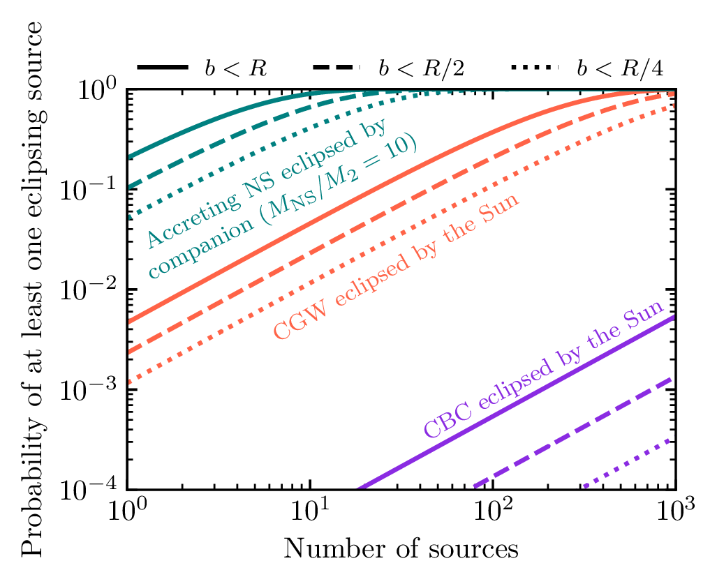
How common are eclipsing gravitational wave sources?

Probability of observing at least one eclipsing source amongst a number of observed sources. Compact binary coalescences (CBCs, shown in purple) are the most rare, continuous gravitational waves (CGWs) eclipsed by the Sun (red) or by a companion (red) are more common. Here we assume companions are stars about a tenth the mass of the neutron star. The number of neutron stars with binary companions is estimated using the COSMIC population synthesis code. Results are shown for eclipses where the gravitational waves get within distance $b$ of the centre of the star. Figure 1 of Marchant et al. (2020).

Continuous gravitational waves are produced by rotating neutron stars. They are pretty much perfect for searching for eclipses. As you might guess from their name, continuous gravitational waves are always there. They happily hum away, sticking to pretty much the same note (they’d get pretty annoying to listen to). Therefore, we can measure them before, during and after an eclipse, and identify any changes due to the gravitational lensing. Furthermore, we’d expect that many neutron stars would be in close binaries, and therefore would be eclipsed by their partner. This would happen each time they orbit, potentially giving us lots of juicy information on these stars. All we need to do is measure the continuous gravitational wave…

The effect of the gravitational lensing by a star is small. We performed detailed calculations for our Sun (using MESA), and found that for the effects to be measurable you would need an extremely loud signal. A signal-to-noise ratio would need to be hundreds during the eclipse for measurement precision to be good enough to notice the imprint of lensing. To map out how things changed as the eclipse progressed, you’d need signal-to-noise ratios many times higher than this. As an eclipse by the Sun is only a small fraction of the time, we’re going to need some really loud signals (at least signal-to-noise ratios of 2500) to see these effects. We will need the next generation of gravitational wave detectors.

We are currently thinking about the next generation of gravitational wave detectors [bonus note]. The leading ideas are successors to LIGO and Virgo: detectors which cover a large range of frequencies to detect many different types of source. These will be expensive (billions of dollars, euros or pounds), and need international collaboration to finance. However, I also like the idea of smaller detectors designed to do one thing really well. Potentially these could be financed by a single national lab. I think eclipsing continuous waves are the perfect source for this—instead of needing a detector sensitive over a wide frequency range, we just need to be sensitive over a really narrow range. We will be able to detect continuous waves before we are able to see the impact of eclipses. Therefore, we’ll know exactly what frequency to tune for. We’ll also know exactly when we need to observe. I think it would be really awesome to have a tunable narrowband detector, which could measure the eclipse of one source, and then be tuned for the next one, and the next. By combining many observations, we could really build up a detailed picture of the Sun. I think this would be an exciting experiment—instrumentalists, put your thinking hats on!

Let’s reach for(the centres of) the stars.

arXiv: 1912.04268 [astro-ph.SR]
Journal: Physical Review D; 101(2):024039(15); 2020
Data release: Eclipses of continuous gravitational waves as a probe of stellar structure
CIERA story: Using gravitational waves to see inside stars
Why does the sun really shine? The Sun is a miasma of incandescent plasma

Bonus notes

Silver lining

Since signals from compact binary coalescences are so unlikely to be eclipsed by a star, we don’t have to worry that our measurements of the source property are being messed up by this type of gravitational lensing distorting the signal. Which is nice.

Prospects with LISA

If you were wondering if we could see these types of eclipses with the space-based gravitational wave observatory LISA, the answer is sadly no. LISA observes lower frequency gravitational waves. Lower frequency means longer wavelength, so long in fact that the wavelength is larger than the size of the Sun! Since the size of the Sun is so small compared to the gravitational wave, it doesn’t leave a same imprint: the wave effectively skips over the gravitational potential.

Second star to the right and straight on ’til morning—Astrophysics white papers

April 20, 2019August 1, 2020 / CPLB / Leave a comment

What will be the next big thing in astronomy? One of the hard things about research is that you often don’t know what you will discover before you embark on an investigation. An idea might work out, or it might not, or along the way you might discover something unexpected which is far more interesting. As you might imagine, this can make laying definite plans difficult…

However, it is important to have plans for research. While you might not be sure of the outcome, it is necessary to weigh the risks and rewards associated with the probable results before you invest your time and taxpayers’ money!

To help with planning and prioritising, researchers in astrophysics often pull together white papers [bonus note]. These are sketches of ideas for future research, arguing why you think they might be interesting. These can then be discussed within the community to help shape the direction of the field. If other scientists find the paper convincing, you can build support which helps push for funding. If there are gaps in the logic, others can point these out to ave you heading the wrong way. This type of consensus building is especially important for large experiments or missions—you don’t want to spend a billion dollars on something unless you’re really sure it is a good idea and lots of people agree.

I have been involved with a few white papers recently. Here are some key ideas for where research should go.

Ground-based gravitational-wave detectors: The next generation

We’ve done some awesome things with Advanced LIGO and Advanced Virgo. In just a couple of years we have revolutionized our understanding of binary black holes. That’s not bad. However, our current gravitational-wave observatories are limited in what they can detect. What amazing things could we achieve with a new generation of detectors?

It can take decades to develop new instruments, therefore it’s important to start thinking about them early. Obviously, what we would most like is an observatory which can detect everything, but that’s not feasible. In this white paper, we pick the questions we most want answered, and see what the requirements for a new detector would be. A design which satisfies these specifications would therefore be a solid choice for future investment.

Binary black holes are the perfect source for ground-based detectors. What do we most want to know about them?

How many mergers are there, and how does the merger rate change over the history of the Universe? We want to know how binary black holes are made. The merger rate encodes lots of information about how to make binaries, and comparing how this evolves compared with the rate at which the Universe forms stars, will give us a deeper understanding of how black holes are made.
What are the properties (masses and spins) of black holes? The merger rate tells us some things about how black holes form, but other properties like the masses, spins and orbital eccentricity complete the picture. We want to make precise measurements for individual systems, and also understand the population.
Where do supermassive black holes come from? We know that stars can collapse to produce stellar-mass black holes. We also know that the centres of galaxies contain massive black holes. Where do these massive black holes come from? Do they grow from our smaller black holes, or do they form in a different way? Looking for intermediate-mass black holes in the gap in-between will tells us whether there is a missing link in the evolution of black holes.

Detection horizon as a function of binary mass for Advanced LIGO, A+, Cosmic Explorer and the Einstein Telescope

The detection horizon (the distance to which sources can be detected) for Advanced LIGO (aLIGO), its upgrade A+, and the proposed Cosmic Explorer (CE) and Einstein Telescope (ET). The horizon is plotted for binaries with equal-mass, nonspinning components. Adapted from Hall & Evans (2019).

What can we do to answer these questions?

Increase sensitivity! Advanced LIGO and Advanced Virgo can detect a $30 M_\odot + 30 M_\odot$ binary out to a redshift of about $z \approx 1$ . The planned detector upgrade A+ will see them out to redshift $z \approx 2$ . That’s pretty impressive, it means we’re covering 10 billion years of history. However, the peak in the Universe’s star formation happens at around $z \approx 2$ , so we’d really like to see beyond this in order to measure how the merger rate evolves. Ideally we would see all the way back to cosmic dawn at $z \approx 20$ when the Universe was only 200 million years old and the first stars light up.
Increase our frequency range! Our current detectors are limited in the range of frequencies they can detect. Pushing to lower frequencies helps us to detect heavier systems. If we want to detect intermediate-mass black holes of $100 M_\odot$ we need this low frequency sensitivity. At the moment, Advanced LIGO could get down to about $10~\mathrm{Hz}$ . The plot below shows the signal from a $100 M_\odot + 100 M_\odot$ binary at $z = 10$ . The signal is completely undetectable at $10~\mathrm{Hz}$ .
The gravitational wave signal from the final stages of inspiral, merger and ringdown of a two 100 solar mass black holes at a redshift of 10. The signal chirps up in frequency. The colour coding shows parts of the signal above different frequencies. Part of Figure 2 of the Binary Black Holes White Paper.
Increase sensitivity and frequency range! Increasing sensitivity means that we will have higher signal-to-noise ratio detections. For these loudest sources, we will be able to make more precise measurements of the source properties. We will also have more detections overall, as we can survey a larger volume of the Universe. Increasing the frequency range means we can observe a longer stretch of the signal (for the systems we currently see). This means it is easier to measure spin precession and orbital eccentricity. We also get to measure a wider range of masses. Putting the improved sensitivity and frequency range together means that we’ll get better measurements of individual systems and a more complete picture of the population.

How much do we need to improve our observatories to achieve our goals? To quantify this, lets consider the boost in sensitivity relative to A+, which I’ll call $\beta_\mathrm{A+}$ . If the questions can be answered with $\beta_\mathrm{A+} = 1$ , then we don’t need anything beyond the currently planned A+. If we need a slightly larger $\beta_\mathrm{A+}$ , we should start investigating extra ways to improve the A+ design. If we need much larger $\beta_\mathrm{A+}$ , we need to think about new facilities.

The plot below shows the boost necessary to detect a binary (with equal-mass nonspinning components) out to a given redshift. With a boost of $\beta_\mathrm{A+} = 10$ (blue line) we can survey black holes around $10 M_\odot$ – $30 M_\odot$ across cosmic time.

Boost to detect a binary of a given mass at a given redshift

The boost factor (relative to A+) $\beta_\mathrm{A+}$ needed to detect a binary with a total mass $M$ out to redshift $z$ . The binaries are assumed to have equal-mass, nonspinning components. The colour scale saturates at $\log_{10} \beta_\mathrm{A+} = 4.5$ . The blue curve highlights the reach at a boost factor of $\beta_\mathrm{A+} = 10$ . The solid and dashed white lines indicate the maximum reach of Cosmic Explorer and the Einstein Telescope, respectively. Part of Figure 1 of the Binary Black Holes White Paper.

The plot above shows that to see intermediate-mass black holes, we do need to completely overhaul the low-frequency sensitivity. What do we need to detect a $100 M_\odot + 100 M_\odot$ binary at $z = 10$ ? If we parameterize the noise spectrum (power spectral density) of our detector as $S_n(f) = S_{10}(f/10~\mathrm{Hz})^\alpha$ with a lower cut-off frequency of $f_\mathrm{min}$ , we can investigate the various possibilities. The plot below shows the possible combinations of parameters which meet of requirements.

Noise curve requirements for intermediate-mass black hole detection

Requirements on the low-frequency noise power spectrum necessary to detect an optimally oriented intermediate-mass binary black hole system with two 100 solar mass components at a redshift of 10. Part of Figure 2 of the Binary Black Holes White Paper.

To build up information about the population of black holes, we need lots of detections. Uncertainties scale inversely with the square root of the number of detections, so you would expect few percent uncertainty after 1000 detections. If we want to see how the population evolves, we need these many per redshift bin! The plot below shows the number of detections per year of observing time for different boost factors. The rate starts to saturate once we detect all the binaries in the redshift range. This is as good as you’ll ever going to get.

Detections per redshift bin as a function of boost factor

Expected rate of binary black hole detections $R_\mathrm{det}$ per redshift bin as a function of A+ boost factor $\beta_\mathrm{A+}$ for three redshift bins. The merging binaries are assumed to be uniformly distributed with a constant merger rate roughly consistent with current observations: the solid line is about the current median, while the dashed and dotted lines are roughly the 90% bounds. Figure 3 of the Binary Black Holes White Paper.

Looking at the plots above, it is clear that A+ is not going to satisfy our requirements. We need something with a boost factor of $\beta_\mathrm{A+} = 10$ : a next-generation observatory. Both the Cosmic Explorer and Einstein Telescope designs do satisfy our goals.

Data is pleased. Credit: Paramount

Title: Deeper, wider, sharper: Next-generation ground-based gravitational-wave observations of binary black holes
arXiv: 1903.09220 [astro-ph.HE]
Contribution level: ☆☆☆☆☆ Leading author
Theme music: Daft Punk

Extreme mass ratio inspirals are awesome

We have seen gravitational waves from a stellar-mass black hole merging with another stellar-mass black hole, can we observe a stellar-mass black hole merging with a massive black hole? Yes, these are a perfect source for a space-based gravitational wave observatory. We call these systems extreme mass-ratio inspirals (or EMRIs, pronounced em-rees, for short) [bonus note].

Having such an extreme mass ratio, with one black hole much bigger than the other, gives EMRIs interesting properties. The number of orbits over the course of an inspiral scales with the mass ratio: the more extreme the mass ratio, the more orbits there are. Each of these gives us something to measure in the gravitational wave signal.

The intricate structure of an EMRI orbit

A short section of an orbit around a spinning black hole. While inspirals last for years, this would represent only a few hours around a black hole of mass $M = 10^6 M_\odot$ . The position is measured in terms of the gravitational radius $r_\mathrm{g} = GM/c^2$ . The innermost stable orbit for this black hole would be about $r_\mathrm{g} = 2.3$ . Part of Figure 1 of the EMRI White Paper.

As EMRIs are so intricate, we can make exquisit measurements of the source properties. These will enable us to:

Measure the masses of both black holes to better than 10% precision
Reconstruct the mass distribution of massive black holes out to redshift $z \gtrsim 4$
Measure massive black hole spins to a precision of better than 0.001, giving us an insight into how they formed
Perform precision tests of the no-hair theorem describing black holes in general relativity, and test alternative theories of gravity in the strong-field regime
Cross-correlate locations with galaxy catalogues to measure the expansion of the Universe

Event rates for EMRIs are currently uncertain: there could be just one per year or thousands. From the rate we can figure out the details of what is going in in the nuclei of galaxies, and what types of objects you find there.

With EMRIs you can unravel mysteries in astrophysics, fundamental physics and cosmology.

Have we sold you that EMRIs are awesome? Well then, what do we need to do to observe them? There is only one currently planned mission which can enable us to study EMRIs: LISA. To maximise the science from EMRIs, we have to support LISA.

As an aspiring scientist, Lisa Simpson is a strong supporter of the LISA mission. Credit: Fox

Title: The unique potential of extreme mass-ratio inspirals for gravitational-wave astronomy
arXiv: 1903.03686 [astro-ph.HE]
Contribution level: ☆☆☆☆☆ Leading author
Theme music: Muse

Bonus notes

White paper vs journal article

Since white papers are proposals for future research, they aren’t as rigorous as usual academic papers. They are really attempts to figure out a good question to ask, rather than being answers. White papers are not usually peer reviewed before publication—the point is that you want everybody to comment on them, rather than just one or two anonymous referees.

Whilst white papers aren’t quite the same class as journal articles, they do still contain some interesting ideas, so I thought they still merit a blog post.

Recycling

I have blogged about EMRIs before, so I won’t go into too much detail here. It was one of my former blog posts which inspired the LISA Science Team to get in touch to ask me to write the white paper.

The O2 Catalogue—It goes up to 11

December 7, 2018January 26, 2020 / CPLB / Leave a comment

The full results of our second advanced-detector observing run (O2) have now been released—we’re pleased to announce four new gravitational wave signals: GW170729, GW170809, GW170818 and GW170823 [bonus note]. These latest observations are all of binary black hole systems. Together, they bring our total to 10 observations of binary black holes, and 1 of a binary neutron star. With more frequent detections on the horizon with our third observing run due to start early 2019, the era of gravitational wave astronomy is truly here.

The population of black holes and neutron stars observed with gravitational waves and with electromagnetic astronomy. You can play with an interactive version of this plot online.

The new detections are largely consistent with our previous findings. GW170809, GW170818 and GW170823 are all similar to our first detection GW150914. Their black holes have masses around 20 to 40 times the mass of our Sun. I would lump GW170104 and GW170814 into this class too. Although there were models that predicted black holes of these masses, we weren’t sure they existed until our gravitational wave observations. The family of black holes continues out of this range. GW151012, GW151226 and GW170608 fall on the lower mass side. These overlap with the population of black holes previously observed in X-ray binaries. Lower mass systems can’t be detected as far away, so we find fewer of these. On the higher end we have GW170729 [bonus note]. Its source is made up of black holes with masses $50.2^{+16.2}_{-10.2} M_\odot$ and $34.0^{+9.1}_{-10.1} M_\odot$ (where $M_\odot$ is the mass of our Sun). The larger black hole is a contender for the most massive black hole we’ve found in a binary (the other probable contender is GW170823’s source, which has a $39.5^{+11.2}_{-6.7} M_\odot$ black hole). We have a big happy family of black holes!

Of the new detections, GW170729, GW170809 and GW170818 were both observed by the Virgo detector as well as the two LIGO detectors. Virgo joined O2 for an exciting August [bonus note], and we decided that the data at the time of GW170729 were good enough to use too. Unfortunately, Virgo wasn’t observing at the time of GW170823. GW170729 and GW170809 are very quiet in Virgo, you can’t confidently say there is a signal there [bonus note]. However, GW170818 is a clear detection like GW170814. Well done Virgo!

Using the collection of results, we can start understand the physics of these binary systems. We will be summarising our findings in a series of papers. A huge amount of work went into these.

The papers

The O2 Catalogue Paper

Title: GWTC-1: A gravitational-wave transient catalog of compact binary mergers observed by LIGO and Virgo during the first and second observing runs
arXiv: 1811.12907 [astro-ph.HE]
Data: Catalogue; Parameter estimation results
Journal: Physical Review X; 9(3):031040(49); 2019
LIGO science summary: GWTC-1: A new catalog of gravitational-wave detections

The paper summarises all our observations of binaries to date. It covers our first and second observing runs (O1 and O2). This is the paper to start with if you want any information. It contains estimates of parameters for all our sources, including updates for previous events. It also contains merger rate estimates for binary neutron stars and binary black holes, and an upper limit for neutron star–black hole binaries. We’re still missing a neutron star–black hole detection to complete the set.

More details: The O2 Catalogue Paper

The O2 Populations Paper

Title: Binary black hole population properties inferred from the first and second observing runs of Advanced LIGO and Advanced Virgo
arXiv: 1811.12940 [astro-ph.HE]
Journal: Astrophysical Journal Letters; 882(2):L24(30); 2019
Data: Population inference results
LIGO science summary: Binary black hole properties inferred from O1 and O2

Using our set of ten binary black holes, we can start to make some statistical statements about the population: the distribution of masses, the distribution of spins, the distribution of mergers over cosmic time. With only ten observations, we still have a lot of uncertainty, and can’t make too many definite statements. However, if you were wondering why we don’t see any more black holes more massive than GW170729, even though we can see these out to significant distances, so are we. We infer that almost all stellar-mass black holes have masses less than $45 M_\odot$ .

More details: The O2 Populations Paper

The O2 Catalogue Paper

Synopsis: O2 Catalogue Paper
Read this if: You want the most up-to-date gravitational results
Favourite part: It’s out! We can tell everyone about our FOUR new detections

This is a BIG paper. It covers our first two observing runs and our main searches for coalescing stellar mass binaries. There will be separate papers going into more detail on searches for other gravitational wave signals.

The instruments

Gravitational wave detectors are complicated machines. You don’t just take them out of the box and press go. We’ll be slowly improving the sensitivity of our detectors as we commission them over the next few years. O2 marks the best sensitivity achieved to date. The paper gives a brief overview of the detector configurations in O2 for both LIGO detectors, which did differ, and Virgo.

During O2, we realised that one source of noise was beam jitter, disturbances in the shape of the laser beam. This was particularly notable in Hanford, where there was a spot on the one of the optics. Fortunately, we are able to measure the effects of this, and hence subtract out this noise. This has now been done for the whole of O2. It makes a big difference! Derek Davis and TJ Massinger won the first LIGO Laboratory Award for Excellence in Detector Characterization and Calibration™ for implementing this noise subtraction scheme (the award citation almost spilled the beans on our new detections). I’m happy that GW170104 now has an increased signal-to-noise ratio, which means smaller uncertainties on its parameters.

The searches

We use three search algorithms in this paper. We have two matched-filter searches (GstLAL and PyCBC). These compare a bank of templates to the data to look for matches. We also use coherent WaveBurst (cWB), which is a search for generic short signals, but here has been tuned to find the characteristic chirp of a binary. Since cWB is more flexible in the signals it can find, it’s slightly less sensitive than the matched-filter searches, but it gives us confidence that we’re not missing things.

The two matched-filter searches both identify all 11 signals with the exception of GW170818, which is only found by GstLAL. This is because PyCBC only flags signals above a threshold in each detector. We’re confident it’s real though, as it is seen in all three detectors, albeit below PyCBC’s threshold in Hanford and Virgo. (PyCBC only looked at signals found in coincident Livingston and Hanford in O2, I suspect they would have found it if they were looking at all three detectors, as that would have let them lower their threshold).

The search pipelines try to distinguish between signal-like features in the data and noise fluctuations. Having multiple detectors is a big help here, although we still need to be careful in checking for correlated noise sources. The background of noise falls off quickly, so there’s a rapid transition between almost-certainly noise to almost-certainly signal. Most of the signals are off the charts in terms of significance, with GW170818, GW151012 and GW170729 being the least significant. GW170729 is found with best significance by cWB, that gives reports a false alarm rate of $1/(50~\mathrm{yr})$ .

Cumulative histogram of results from GstLAL (top left), PyCBC (top right) and cWB (bottom). The expected background is shown as the dashed line and the shaded regions give Poisson uncertainties. The search results are shown as the solid red line and named gravitational-wave detections are shown as blue dots. More significant results are further to the right of the plot. Fig. 2 and Fig. 3 of the O2 Catalogue Paper.

The false alarm rate indicates how often you would expect to find something at least as signal like if you were to analyse a stretch of data with the same statistical properties as the data considered, assuming that they is only noise in the data. The false alarm rate does not fold in the probability that there are real gravitational waves occurring at some average rate. Therefore, we need to do an extra layer of inference to work out the probability that something flagged by a search pipeline is a real signal versus is noise.

The results of this calculation is given in Table IV. GW170729 has a 94% probability of being real using the cWB results, 98% using the GstLAL results, but only 52% according to PyCBC. Therefore, if you’re feeling bold, you might, say, only wager the entire economy of the UK on it being real.

We also list the most marginal triggers. These all have probabilities way below being 50% of being real: if you were to add them all up you wouldn’t get a total of 1 real event. (In my professional opinion, they are garbage). However, if you want to check for what we might have missed, these may be a place to start. Some of these can be explained away as instrumental noise, say scattered light. Others show no obvious signs of disturbance, so are probably just some noise fluctuation.

The source properties

We give updated parameter estimates for all 11 sources. These use updated estimates of calibration uncertainty (which doesn’t make too much difference), improved estimate of the noise spectrum (which makes some difference to the less well measured parameters like the mass ratio), the cleaned data (which helps for GW170104), and our most currently complete waveform models [bonus note].

This plot shows the masses of the two binary components (you can just make out GW170817 down in the corner). We use the convention that the more massive of the two is $m_1$ and the lighter is $m_2$ . We are now really filling in the mass plot! Implications for the population of black holes are discussed in the Populations Paper.

Estimated masses for the two binary objects for each of the events in O1 and O2. From lowest chirp mass (left; red) to highest (right; purple): GW170817 (solid), GW170608 (dashed), GW151226 (solid), GW151012 (dashed), GW170104 (solid), GW170814 (dashed), GW170809 (dashed), GW170818 (dashed), GW150914 (solid), GW170823 (dashed), GW170729 (solid). The contours mark the 90% credible regions. The grey area is excluded from our convention on masses. Part of Fig. 4 of the O2 Catalogue Paper. The mass ratio is $q = m_2/m_1$ .

As well as mass, black holes have a spin. For the final black hole formed in the merger, these spins are always around 0.7, with a little more or less depending upon which way the spins of the two initial black holes were pointing. As well as being probably the most most massive, GW170729’s could have the highest final spin! It is a record breaker. It radiated a colossal $4.8^{+1.7}_{-1.7} M_\odot$ worth of energy in gravitational waves [bonus note].

Estimated final masses and spins for each of the binary black hole events in O1 and O2. From lowest chirp mass (left; red–orange) to highest (right; purple): GW170608 (dashed), GW151226 (solid), GW151012 (dashed), GW170104 (solid), GW170814 (dashed), GW170809 (dashed), GW170818 (dashed), GW150914 (solid), GW170823 (dashed), GW170729 (solid). The contours mark the 90% credible regions. Part of Fig. 4 of the O2 Catalogue Paper.

There is considerable uncertainty on the spins as there are hard to measure. The best combination to pin down is the effective inspiral spin parameter $\chi_\mathrm{eff}$ . This is a mass weighted combination of the spins which has the most impact on the signal we observe. It could be zero if the spins are misaligned with each other, point in the orbital plane, or are zero. If it is non-zero, then it means that at least one black hole definitely has some spin. GW151226 and GW170729 have $\chi_\mathrm{eff} > 0$ with more than 99% probability. The rest are consistent with zero. The spin distribution for GW170104 has tightened up for GW170104 as its signal-to-noise ratio has increased, and there’s less support for negative $\chi_\mathrm{eff}$ , but there’s been no move towards larger positive $\chi_\mathrm{eff}$ .

For our analysis, we use two different waveform models to check for potential sources of systematic error. They agree pretty well. The spins are where they show most difference (which makes sense, as this is where they differ in terms of formulation). For GW151226, the effective precession waveform IMRPhenomPv2 gives $0.20^{+0.18}_{-0.08}$ and the full precession model gives $0.15^{+0.25}_{-0.11}$ and extends to negative $\chi_\mathrm{eff}$ . I panicked a little bit when I first saw this, as GW151226 having a non-zero spin was one of our headline results when first announced. Fortunately, when I worked out the numbers, all our conclusions were safe. The probability of $\chi_\mathrm{eff} < 0$ is less than 1%. In fact, we can now say that at least one spin is greater than $0.28$ at 99% probability compared with $0.2$ previously, because the full precession model likes spins in the orbital plane a bit more. Who says data analysis can’t be thrilling?

Our measurement of $\chi_\mathrm{eff}$ tells us about the part of the spins aligned with the orbital angular momentum, but not in the orbital plane. In general, the in-plane components of the spin are only weakly constrained. We basically only get back the information we put in. The leading order effects of in-plane spins is summarised by the effective precession spin parameter $\chi_\mathrm{p}$ . The plot below shows the inferred distributions for $\chi_\mathrm{p}$ . The left half for each event shows our results, the right shows our prior after imposed the constraints on spin we get from $\chi_\mathrm{eff}$ . We get the most information for GW151226 and GW170814, but even then it’s not much, and we generally cover the entire allowed range of values.

All effective precession spin parameters

Estimated effective inspiral spin parameters for each of the events in O1 and O2. From lowest chirp mass (left; red) to highest (right; purple): GW170817, GW170608, GW151226, GW151012, GW170104, GW170814, GW170809, GW170818, GW150914, GW170823, GW170729. The left (coloured) part of the plot shows the posterior distribution; the right (white) shows the prior conditioned by the effective inspiral spin parameter constraints. Part of Fig. 5 of the O2 Catalogue Paper.

One final measurement which we can make (albeit with considerable uncertainty) is the distance to the source. The distance influences how loud the signal is (the further away, the quieter it is). This also depends upon the inclination of the source (a binary edge-on is quieter than a binary face-on/off). Therefore, the distance is correlated with the inclination and we end up with some butterfly-like plots. GW170729 is again a record setter. It comes from a luminosity distance of $2.84^{+1.40}_{-1.36}~\mathrm{Gpc}$ away. That means it has travelled across the Universe for $3.2$ – $6.2$ billion years—it potentially started its journey before the Earth formed!

Estimated luminosity distances and orbital inclinations for each of the events in O1 and O2. From lowest chirp mass (left; red) to highest (right; purple): GW170817 (solid), GW170608 (dashed), GW151226 (solid), GW151012 (dashed), GW170104 (solid), GW170814 (dashed), GW170809 (dashed), GW170818 (dashed), GW150914 (solid), GW170823 (dashed), GW170729 (solid). The contours mark the 90% credible regions.An inclination of zero means that we’re looking face-on along the direction of the total angular momentum, and inclination of $\pi/2$ means we’re looking edge-on perpendicular to the angular momentum. Part of Fig. 7 of the O2 Catalogue Paper.

Waveform reconstructions

To check our results, we reconstruct the waveforms from the data to see that they match our expectations for binary black hole waveforms (and there’s not anything extra there). To do this, we use unmodelled analyses which assume that there is a coherent signal in the detectors: we use both cWB and BayesWave. The results agree pretty well. The reconstructions beautifully match our templates when the signal is loud, but, as you might expect, can resolve the quieter details. You’ll also notice the reconstructions sometimes pick up a bit of background noise away from the signal. This gives you and idea of potential fluctuations.

Time–frequency maps and reconstructed signal waveforms for the binary black holes. For each event we show the results from the detector where the signal was loudest. The left panel for each shows the time–frequency spectrogram with the upward-sweeping chip. The right show waveforms: blue the modelled waveforms used to infer parameters (LALInf; top panel); the red wavelet reconstructions (BayesWave; top panel); the black is the maximum-likelihood cWB reconstruction (bottom panel), and the green (bottom panel) shows reconstructions for simulated similar signals. I think the agreement is pretty good! All the data have been whitened as this is how we perform the statistical analysis of our data. Fig. 10 of the O2 Catalogue Paper.

I still think GW170814 looks like a slug. Some people think they look like crocodiles.

We’ll be doing more tests of the consistency of our signals with general relativity in a future paper.

Merger rates

Given all our observations now, we can set better limits on the merger rates. Going from the number of detections seen to the number merger out in the Universe depends upon what you assume about the mass distribution of the sources. Therefore, we make a few different assumptions.

For binary black holes, we use (i) a power-law model for the more massive black hole similar to the initial mass function of stars, with a uniform distribution on the mass ratio, and (ii) use uniform-in-logarithmic distribution for both masses. These were designed to bracket the two extremes of potential distributions. With our observations, we’re starting to see that the true distribution is more like the power-law, so I expect we’ll be abandoning these soon. Taking the range of possible values from our calculations, the rate is in the range of $9.7$ – $101~\mathrm{Gpc^{-3}\,yr^{-1}}$ for black holes between $5 M_\odot$ and $50 M_\odot$ [bonus note].

For binary neutron stars, which are perhaps more interesting astronomers, we use a uniform distribution of masses between $0.8 M_\odot$ and $2.3 M_\odot$ , and a Gaussian distribution to match electromagnetic observations. We find that these bracket the range $97$ – $4440~\mathrm{Gpc^{-3}\,yr^{-1}}$ . This larger than are previous range, as we hadn’t considered the Gaussian distribution previously.

90% upper limits for neutron star–black hole binaries. Three black hole masses were tried and two spin distributions. Results are shown for the two matched-filter search algorithms. Fig. 14 of the O2 Catalogue Paper.

Finally, what about neutron star–black holes? Since we don’t have any detections, we can only place an upper limit. This is a maximum of $610~\mathrm{Gpc^{-3}\,yr^{-1}}$ . This is about a factor of 2 better than our O1 results, and is starting to get interesting!

We are sure to discover lots more in O3… [bonus note].

The O2 Populations Paper

Synopsis: O2 Populations Paper
Read this if: You want the best family portrait of binary black holes
Favourite part: A maximum black hole mass?

Each detection is exciting. However, we can squeeze even more science out of our observations by looking at the entire population. Using all 10 of our binary black hole observations, we start to trace out the population of binary black holes. Since we still only have 10, we can’t yet be too definite in our conclusions. Our results give us some things to ponder, while we are waiting for the results of O3. I think now is a good time to start making some predictions.

We look at the distribution of black hole masses, black hole spins, and the redshift (cosmological time) of the mergers. The black hole masses tell us something about how you go from a massive star to a black hole. The spins tell us something about how the binaries form. The redshift tells us something about how these processes change as the Universe evolves. Ideally, we would look at these all together allowing for mixtures of binary black holes formed through different means. Given that we only have a few observations, we stick to a few simple models.

To work out the properties of the population, we perform a hierarchical analysis of our 10 binary black holes. We infer the properties of the individual systems, assuming that they come from a given population, and then see how well that population fits our data compared with a different distribution.

In doing this inference, we account for selection effects. Our detectors are not equally sensitive to all sources. For example, nearby sources produce louder signals and we can’t detect signals that are too far away, so if you didn’t account for this you’d conclude that binary black holes only merged in the nearby Universe. Perhaps less obvious is that we are not equally sensitive to all source masses. More massive binaries produce louder signals, so we can detect these further way than lighter binaries (up to the point where these binaries are so high mass that the signals are too low frequency for us to easily spot). This is why we detect more binary black holes than binary neutron stars, even though there are more binary neutron stars out here in the Universe.

Masses

When looking at masses, we try three models of increasing complexity:

Model A is a simple power law for the mass of the more massive black hole $m_1$ . There’s no real reason to expect the masses to follow a power law, but the masses of stars when they form do, and astronomers generally like power laws as they’re friendly, so its a sensible thing to try. We fit for the power-law index. The power law goes from a lower limit of $5 M_\odot$ to an upper limit which we also fit for. The mass of the lighter black hole $m_2$ is assumed to be uniformly distributed between $5 M_\odot$ and the mass of the other black hole.
Model B is the same power law, but we also allow the lower mass limit to vary from $5 M_\odot$ . We don’t have much sensitivity to low masses, so this lower bound is restricted to be above $5 M_\odot$ . I’d be interested in exploring lower masses in the future. Additionally, we allow the mass ratio $q = m_2/m_1$ of the black holes to vary, trying $q^{\beta_q}$ instead of Model A’s $q^0$ .
Model C has the same power law, but now with some smoothing at the low-mass end, rather than a sharp turn-on. Additionally, it includes a Gaussian component towards higher masses. This was inspired by the possibility of pulsational pair-instability supernova causing a build up of black holes at certain masses: stars which undergo this lose extra mass, so you’d end up with lower mass black holes than if the stars hadn’t undergone the pulsations. The Gaussian could fit other effects too, for example if there was a secondary formation channel, or just reflect that the pure power law is a bad fit.

In allowing the mass distributions to vary, we find overall rates which match pretty well those we obtain with our main power-law rates calculation included in the O2 Catalogue Paper, higher than with the main uniform-in-log distribution.

The fitted mass distributions are shown in the plot below. The error bars are pretty broad, but I think the models agree on some broad features: there are more light black holes than heavy black holes; the minimum black hole mass is below about $9 M_\odot$ , but we can’t place a lower bound on it; the maximum black hole mass is above about $35 M_\odot$ and below about $50 M_\odot$ , and we prefer black holes to have more similar masses than different ones. The upper bound on the black hole minimum mass, and the lower bound on the black hole upper mass are set by the smallest and biggest black holes we’ve detected, respectively.

Binary black hole merger rate as a function of the primary mass ( $m_1$ ; top) and mass ratio ( $q$ ; bottom). The solid lines and bands show the medians and 90% intervals. The dashed line shows the posterior predictive distribution: our expectation for future observations averaging over our uncertainties. Fig. 2 of the O2 Populations Paper.

That there does seem to be a drop off at higher masses is interesting. There could be something which stops stars forming black holes in this range. It has been proposed that there is a mass gap due to pair instability supernovae. These explosions completely disrupt their progenitor stars, leaving nothing behind. (I’m not sure if they are accompanied by a flash of green light). You’d expect this to kick for black holes of about $50$ – $60 M_\odot$ . We infer that 99% of merging black holes have masses below $44.0 M_\odot$ with Model A, $41.8 M_\odot$ with Model B, and $41.8 M_\odot$ with Model C. Therefore, our results are not inconsistent with a mass gap. However, we don’t really have enough evidence to be sure.

We can compare how well each of our three models fits the data by looking at their Bayes factors. These naturally incorporate the complexity of the models: models with more parameters (which can be more easily tweaked to match the data) are penalised so that you don’t need to worry about overfitting. We have a preference for Model C. It’s not strong, but I think good evidence that we can’t use a simple power law.

Spins

To model the spins:

For the magnitude, we assume a beta distribution. There’s no reason for this, but these are convenient distributions for things between 0 and 1, which are the limits on black hole spin (0 is nonspinning, 1 is as fast as you can spin). We assume that both spins are drawn from the same distribution.
For the spin orientations, we use a mix of an isotropic distribution and a Gaussian centred on being aligned with the orbital angular momentum. You’d expect an isotropic distribution if binaries were assembled dynamically, and perhaps something with spins generally aligned with each other if the binary evolved in isolation.

We don’t get any useful information on the mixture fraction. Looking at the spin magnitudes, we have a preference towards smaller spins, but still have support for large spins. The more misaligned spins are, the larger the spin magnitudes can be: for the isotropic distribution, we have support all the way up to maximal values.

Parametric and binned spin magnitude distributions

Inferred spin magnitude distributions. The left shows results for the parametric distribution, assuming a mixture of almost aligned and isotropic spin, with the median (solid), 50% and 90% intervals shaded, and the posterior predictive distribution as the dashed line. Results are included both for beta distributions which can be singular at 0 and 1, and with these excluded. Model V is a very low spin model shown for comparison. The right shows a binned reconstruction of the distribution for aligned and isotropic distributions, showing the median and 90% intervals. Fig. 8 of the O2 Populations Paper.

Since spins are harder to measure than masses, it is not surprising that we can’t make strong statements yet. If we were to find something with definitely negative $\chi_\mathrm{eff}$ , we would be able to deduce that spins can be seriously misaligned.

Redshift evolution

As a simple model of evolution over cosmological time, we allow the merger rate to evolve as $(1+z)^\lambda$ . That’s right, another power law! Since we’re only sensitive to relatively small redshifts for the masses we detect ( $z < 1$ ), this gives a good approximation to a range of different evolution schemes.

Evolution of the binary black hole merger rate (blue), showing median, 50% and 90% intervals. For comparison, a non-evolving rate calculated using Model B is shown too. Fig. 6 of the O2 Populations Paper.

We find that we prefer evolutions that increase with redshift. There’s an 88% probability that $\lambda > 0$ , but we’re still consistent with no evolution. We might expect rate to increase as star formation was higher bach towards $z =2$ . If we can measure the time delay between forming stars and black holes merging, we could figure out what happens to these systems in the meantime.

The local merger rate is broadly consistent with what we infer with our non-evolving distributions, but is a little on the lower side.

Bonus notes

Naming

Gravitational waves are named as GW-year-month-day, so our first observation from 14 September 2015 is GW150914. We realise that this convention suffers from a Y2K-style bug, but by the time we hit 2100, we’ll have so many detections we’ll need a new scheme anyway.

Previously, we had a second designation for less significant potential detections. They were LIGO–Virgo Triggers (LVT), the one example being LVT151012. No-one was really happy with this designation, but it stems from us being cautious with our first announcement, and not wishing to appear over bold with claiming we’d seen two gravitational waves when the second wasn’t that certain. Now we’re a bit more confident, and we’ve decided to simplify naming by labelling everything a GW on the understanding that this now includes more uncertain events. Under the old scheme, GW170729 would have been LVT170729. The idea is that the broader community can decide which events they want to consider as real for their own studies. The current condition for being called a GW is that the probability of it being a real astrophysical signal is at least 50%. Our 11 GWs are safely above that limit.

The naming change has hidden the fact that now when we used our improved search pipelines, the significance of GW151012 has increased. It would now be a GW even under the old scheme. Congratulations LVT151012, I always believed in you!

Is it of extraterrestrial origin, or is it just a blurry figure? GW151012: the truth is out there!.

Burning bright

We are lacking nicknames for our new events. They came in so fast that we kind of lost track. Ilya Mandel has suggested that GW170729 should be the Tiger, as it happened on the International Tiger Day. Since tigers are the biggest of the big cats, this seems apt.

Carl-Johan Haster argues that LIGO+tiger = Liger. Since ligers are even bigger than tigers, this seems like an excellent case to me! I’d vote for calling the bigger of the two progenitor black holes GW170729-tiger, the smaller GW170729-lion, and the final black hole GW17-729-liger.

Suggestions for other nicknames are welcome, leave your ideas in the comments.

August 2017—Something fishy or just Poisson statistics?

The final few weeks of O2 were exhausting. I was trying to write job applications at the time, and each time I sat down to work on my research proposal, my phone went off with another alert. You may be wondering about was special about August. Some have hypothesised that it is because Aaron Zimmerman, my partner for the analysis of GW170104, was on the Parameter Estimation rota to analyse the last few weeks of O2. The legend goes that Aaron is especially lucky as he was bitten by a radioactive Leprechaun. I can neither confirm nor deny this. However, I make a point of playing any lottery numbers suggested by him.

A slightly more mundane explanation is that August was when the detectors were running nice and stably. They were observing for a large fraction of the time. LIGO Livingston reached its best sensitivity at this time, although it was less happy for Hanford. We often quantify the sensitivity of our detectors using their binary neutron star range, the average distance they could see a binary neutron star system with a signal-to-noise ratio of 8. If this increases by a factor of 2, you can see twice as far, which means you survey 8 times the volume. This cubed factor means even small improvements can have a big impact. The LIGO Livingston range peak a little over $100~\mathrm{Mpc}$ . We’re targeting at least $120~\mathrm{Mpc}$ for O3, so August 2017 gives an indication of what you can expect.

Binary neutron star range for the instruments across O2. The break around week 3 was for the holidays (We did work Christmas 2015). The break at week 23 was to tune-up the instruments, and clean the mirrors. At week 31 there was an earthquake in Montana, and the Hanford sensitivity didn’t recover by the end of the run. Part of Fig. 1 of the O2 Catalogue Paper.

Of course, in the case of GW170817, we just got lucky.

Sign errors

GW170809 was the first event we identified with Virgo after it joined observing. The signal in Virgo is very quiet. We actually got better results when we flipped the sign of the Virgo data. We were just starting to get paranoid when GW170814 came along and showed us that everything was set up right at Virgo. When I get some time, I’d like to investigate how often this type of confusion happens for quiet signals.

SEOBNRv3

One of the waveforms, which includes the most complete prescription of the precession of the spins of the black holes, we use in our analysis goes by the technical name of SEOBNRv3. It is extremely computationally expensive. Work has been done to improve that, but this hasn’t been implemented in our reviewed codes yet. We managed to complete an analysis for the GW170104 Discovery Paper, which was a huge effort. I said then to not expect it for all future events. We did it for all the black holes, even for the lowest mass sources which have the longest signals. I was responsible for GW151226 runs (as well as GW170104) and I started these back at the start of the summer. Eve Chase put in a heroic effort to get GW170608 results, we pulled out all the stops for that.

Thanksgiving

I have recently enjoyed my first Thanksgiving in the US. I was lucky enough to be hosted for dinner by Shane Larson and his family (and cats). I ate so much I thought I might collapse to a black hole. Apparently, a Thanksgiving dinner can be 3000–4500 calories. That sounds like a lot, but the merger of GW170729 would have emitted about $5 \times 10^{40}$ times more energy. In conclusion, I don’t need to go on a diet.

Confession

We cheated a little bit in calculating the rates. Roughly speaking, the merger rate is given by

$\displaystyle R = \frac{N}{\langle VT\rangle}$ ,

where $N$ is the number of detections and $\langle VT\rangle$ is the amount of volume and time we’ve searched. You expect to detect more events if you increase the sensitivity of the detectors (and hence $V$ ), or observer for longer (and hence increase $T$ ). In our calculation, we included GW170608 in $N$ , even though it was found outside of standard observing time. Really, we should increase $\langle VT\rangle$ to factor in the extra time outside of standard observing time when we could have made a detection. This is messy to calculate though, as there’s not really a good way to check this. However, it’s only a small fraction of the time (so the extra $T$ should be small), and for much of the sensitivity of the detectors will be poor (so $V$ will be small too). Therefore, we estimated any bias from neglecting this is smaller than our uncertainty from the calibration of the detectors, and not worth worrying about.

New sources

We saw our first binary black hole shortly after turning on the Advanced LIGO detectors. We saw our first binary neutron star shortly after turning on the Advanced Virgo detector. My money is therefore on our first neutron star–black hole binary shortly after we turn on the KAGRA detector. Because science…

Accuracy of inference on the physics of binary evolution from gravitational-wave observations

June 11, 2018July 9, 2019 / CPLB / Leave a comment

Gravitational-wave astronomy lets us observing binary black holes. These systems, being made up of two black holes, are pretty difficult to study by any other means. It has long been argued that with this new information we can unravel the mysteries of stellar evolution. Just as a palaeontologist can discover how long-dead animals lived from their bones, we can discover how massive stars lived by studying their black hole remnants. In this paper, we quantify how much we can really learn from this black hole palaeontology—after 1000 detections, we should pin down some of the most uncertain parameters in binary evolution to a few percent precision.

Life as a binary

There are many proposed ways of making a binary black hole. The current leading contender is isolated binary evolution: start with a binary star system (most stars are in binaries or higher multiples, our lonesome Sun is a little unusual), and let the stars evolve together. Only a fraction will end with black holes close enough to merge within the age of the Universe, but these would be the sources of the signals we see with LIGO and Virgo. We consider this isolated binary scenario in this work [bonus note].

Now, you might think that with stars being so fundamentally important to astronomy, and with binary stars being so common, we’d have the evolution of binaries figured out by now. It turns out it’s actually pretty messy, so there’s lots of work to do. We consider constraining four parameters which describe the bits of binary physics which we are currently most uncertain of:

Black hole natal kicks—the push black holes receive when they are born in supernova explosions. We now the neutron stars get kicks, but we’re less certain for black holes [bonus note].
Common envelope efficiency—one of the most intricate bits of physics about binaries is how mass is transferred between stars. As they start exhausting their nuclear fuel they puff up, so material from the outer envelope of one star may be stripped onto the other. In the most extreme cases, a common envelope may form, where so much mass is piled onto the companion, that both stars live in a single fluffy envelope. Orbiting inside the envelope helps drag the two stars closer together, bringing them closer to merging. The efficiency determines how quickly the envelope becomes unbound, ending this phase.
Mass loss rates during the Wolf–Rayet (not to be confused with Wolf 359) and luminous blue variable phases–stars lose mass through out their lives, but we’re not sure how much. For stars like our Sun, mass loss is low, there is enough to gives us the aurora, but it doesn’t affect the Sun much. For bigger and hotter stars, mass loss can be significant. We consider two evolutionary phases of massive stars where mass loss is high, and currently poorly known. Mass could be lost in clumps, rather than a smooth stream, making it difficult to measure or simulate.

We use parameters describing potential variations in these properties are ingredients to the COMPAS population synthesis code. This rapidly (albeit approximately) evolves a population of stellar binaries to calculate which will produce merging binary black holes.

The question is now which parameters affect our gravitational-wave measurements, and how accurately we can measure those which do?

Merger rate with redshift and chirp mass

Binary black hole merger rate at three different redshifts $z$ as calculated by COMPAS. We show the rate in 30 different chirp mass bins for our default population parameters. The caption gives the total rate for all masses. Figure 2 of Barrett et al. (2018)

Gravitational-wave observations

For our deductions, we use two pieces of information we will get from LIGO and Virgo observations: the total number of detections, and the distributions of chirp masses. The chirp mass is a combination of the two black hole masses that is often well measured—it is the most important quantity for controlling the inspiral, so it is well measured for low mass binaries which have a long inspiral, but is less well measured for higher mass systems. In reality we’ll have much more information, so these results should be the minimum we can actually do.

We consider the population after 1000 detections. That sounds like a lot, but we should have collected this many detections after just 2 or 3 years observing at design sensitivity. Our default COMPAS model predicts 484 detections per year of observing time! Honestly, I’m a little scared about having this many signals…

For a set of population parameters (black hole natal kick, common envelope efficiency, luminous blue variable mass loss and Wolf–Rayet mass loss), COMPAS predicts the number of detections and the fraction of detections as a function of chirp mass. Using these, we can work out the probability of getting the observed number of detections and fraction of detections within different chirp mass ranges. This is the likelihood function: if a given model is correct we are more likely to get results similar to its predictions than further away, although we expect their to be some scatter.

If you like equations, the from of our likelihood is explained in this bonus note. If you don’t like equations, there’s one lurking in the paragraph below. Just remember, that it can’t see you if you don’t move. It’s OK to skip the equation.

To determine how sensitive we are to each of the population parameters, we see how the likelihood changes as we vary these. The more the likelihood changes, the easier it should be to measure that parameter. We wrap this up in terms of the Fisher information matrix. This is defined as

$\displaystyle F_{ij} = -\left\langle\frac{\partial^2\ln \mathcal{L}(\mathcal{D}|\left\{\lambda\right\})}{\partial \lambda_i \partial\lambda_j}\right\rangle$ ,

where $\mathcal{L}(\mathcal{D}|\left\{\lambda\right\})$ is the likelihood for data $\mathcal{D}$ (the number of observations and their chirp mass distribution in our case), $\left\{\lambda\right\}$ are our parameters (natal kick, etc.), and the angular brackets indicate the average over the population parameters. In statistics terminology, this is the variance of the score, which I think sounds cool. The Fisher information matrix nicely quantifies how much information we can lean about the parameters, including the correlations between them (so we can explore degeneracies). The inverse of the Fisher information matrix gives a lower bound on the covariance matrix (the multidemensional generalisation of the variance in a normal distribution) for the parameters $\left\{\lambda\right\}$ . In the limit of a large number of detections, we can use the Fisher information matrix to estimate the accuracy to which we measure the parameters [bonus note].

We simulated several populations of binary black hole signals, and then calculate measurement uncertainties for our four population uncertainties to see what we could learn from these measurements.

Results

Using just the rate information, we find that we can constrain a combination of the common envelope efficiency and the Wolf–Rayet mass loss rate. Increasing the common envelope efficiency ends the common envelope phase earlier, leaving the binary further apart. Wider binaries take longer to merge, so this reduces the merger rate. Similarly, increasing the Wolf–Rayet mass loss rate leads to wider binaries and smaller black holes, which take longer to merge through gravitational-wave emission. Since the two parameters have similar effects, they are anticorrelated. We can increase one and still get the same number of detections if we decrease the other. There’s a hint of a similar correlation between the common envelope efficiency and the luminous blue variable mass loss rate too, but it’s not quite significant enough for us to be certain it’s there.

Correaltions between population parameters

Fisher information matrix estimates for fractional measurement precision of the four population parameters: the black hole natal kick $\sigma_\mathrm{kick}$ , the common envelope efficiency $\alpha_\mathrm{CE}$ , the Wolf–Rayet mass loss rate $f_\mathrm{WR}$ , and the luminous blue variable mass loss rate $f_\mathrm{LBV}$ . There is an anticorrealtion between $f_\mathrm{WR}$ and $\alpha_\mathrm{CE}$ , and hints at a similar anticorrelation between $f_|mathrm{LBV}$ and $\alpha_\mathrm{CE}$ . We show 1500 different realisations of the binary population to give an idea of scatter. Figure 6 of Barrett et al. (2018)

Adding in the chirp mass distribution gives us more information, and improves our measurement accuracies. The fraction uncertainties are about 2% for the two mass loss rates and the common envelope efficiency, and about 5% for the black hole natal kick. We’re less sensitive to the natal kick because the most massive black holes don’t receive a kick, and so are unaffected by the kick distribution [bonus note]. In any case, these measurements are exciting! With this type of precision, we’ll really be able to learn something about the details of binary evolution.

Standard deviation of measurements of population parameters

Measurement precision for the four population parameters after 1000 detections. We quantify the precision with the standard deviation estimated from the Fisher inforamtion matrix. We show results from 1500 realisations of the population to give an idea of scatter. Figure 5 of Barrett et al. (2018)

The accuracy of our measurements will improve (on average) with the square root of the number of gravitational-wave detections. So we can expect 1% measurements after about 4000 observations. However, we might be able to get even more improvement by combining constraints from other types of observation. Combining different types of observation can help break degeneracies. I’m looking forward to building a concordance model of binary evolution, and figuring out exactly how massive stars live their lives.

arXiv: 1711.06287 [astro-ph.HE]
Journal: Monthly Notices of the Royal Astronomical Society; 477(4):4685–4695; 2018
Favourite dinosaur: Professor Science

Bonus notes

Channel selection

In practise, we will need to worry about how binary black holes are formed, via isolated evolution or otherwise, before inferring the parameters describing binary evolution. This makes the problem more complicated. Some parameters, like mass loss rates or black hole natal kicks, might be common across multiple channels, while others are not. There are a number of ways we might be able to tell different formation mechanisms apart, such as by using spin measurements.

Kick distribution

We model the supernova kicks $v_\mathrm{kick}$ as following a Maxwell–Boltzmann distribution,

$\displaystyle p(v_\mathrm{kick}) = \sqrt{\frac{2}{\pi}} \frac{v_\mathrm{kick}^2}{\sigma_\mathrm{kick}^3} \exp\left(\frac{-v_\mathrm{kick}^2}{2\sigma_\mathrm{kick}^2}\right)$ ,

where $\sigma_\mathrm{kick}$ is the unknown population parameter. The natal kick received by the black hole $v^*_\mathrm{kick}$ is not the same as this, however, as we assume some of the material ejected by the supernova falls back, reducing the over kick. The final natal kick is

$v^*_\mathrm{kick} = (1-f_\mathrm{fb})v_\mathrm{kick}$ ,

where $f_\mathrm{fb}$ is the fraction that falls back, taken from Fryer et al. (2012). The fraction is greater for larger black holes, so the biggest black holes get no kicks. This means that the largest black holes are unaffected by the value of $\sigma_\mathrm{kick}$ .

The likelihood

In this analysis, we have two pieces of information: the number of detections, and the chirp masses of the detections. The first is easy to summarise with a single number. The second is more complicated, and we consider the fraction of events within different chirp mass bins.

Our COMPAS model predicts the merger rate $\mu$ and the probability of falling in each chirp mass bin $p_k$ (we factor measurement uncertainty into this). Our observations are the the total number of detections $N_\mathrm{obs}$ and the number in each chirp mass bin $c_k$ ( $N_\mathrm{obs} = \sum_k c_k$ ). The likelihood is the probability of these observations given the model predictions. We can split the likelihood into two pieces, one for the rate, and one for the chirp mass distribution,

$\mathcal{L} = \mathcal{L}_\mathrm{rate} \times \mathcal{L}_\mathrm{mass}$ .

For the rate likelihood, we need the probability of observing $N_\mathrm{obs}$ given the predicted rate $\mu$ . This is given by a Poisson distribution,

$\displaystyle \mathcal{L}_\mathrm{rate} = \exp(-\mu t_\mathrm{obs}) \frac{(\mu t_\mathrm{obs})^{N_\mathrm{obs}}}{N_\mathrm{obs}!}$ ,

where $t_\mathrm{obs}$ is the total observing time. For the chirp mass likelihood, we the probability of getting a number of detections in each bin, given the predicted fractions. This is given by a multinomial distribution,

$\displaystyle \mathcal{L}_\mathrm{mass} = \frac{N_\mathrm{obs}!}{\prod_k c_k!} \prod_k p_k^{c_k}$ .

These look a little messy, but they simplify when you take the logarithm, as we need to do for the Fisher information matrix.

When we substitute in our likelihood into the expression for the Fisher information matrix, we get

$\displaystyle F_{ij} = \mu t_\mathrm{obs} \left[ \frac{1}{\mu^2} \frac{\partial \mu}{\partial \lambda_i} \frac{\partial \mu}{\partial \lambda_j} + \sum_k\frac{1}{p_k} \frac{\partial p_k}{\partial \lambda_i} \frac{\partial p_k}{\partial \lambda_j} \right]$ .

Conveniently, although we only need to evaluate first-order derivatives, even though the Fisher information matrix is defined in terms of second derivatives. The expected number of events is $\langle N_\mathrm{obs} \rangle = \mu t_\mathrm{obs}$ . Therefore, we can see that the measurement uncertainty defined by the inverse of the Fisher information matrix, scales on average as $N_\mathrm{obs}^{-1/2}$ .

For anyone worrying about using the likelihood rather than the posterior for these estimates, the high number of detections [bonus note] should mean that the information we’ve gained from the data overwhelms our prior, meaning that the shape of the posterior is dictated by the shape of the likelihood.

Interpretation of the Fisher information matrix

As an alternative way of looking at the Fisher information matrix, we can consider the shape of the likelihood close to its peak. Around the maximum likelihood point, the first-order derivatives of the likelihood with respect to the population parameters is zero (otherwise it wouldn’t be the maximum). The maximum likelihood values of $N_\mathrm{obs} = \mu t_\mathrm{obs}$ and $c_k = N_\mathrm{obs} p_k$ are the same as their expectation values. The second-order derivatives are given by the expression we have worked out for the Fisher information matrix. Therefore, in the region around the maximum likelihood point, the Fisher information matrix encodes all the relevant information about the shape of the likelihood.

So long as we are working close to the maximum likelihood point, we can approximate the distribution as a multidimensional normal distribution with its covariance matrix determined by the inverse of the Fisher information matrix. Our results for the measurement uncertainties are made subject to this approximation (which we did check was OK).

Approximating the likelihood this way should be safe in the limit of large $N_\mathrm{obs}$ . As we get more detections, statistical uncertainties should reduce, with the peak of the distribution homing in on the maximum likelihood value, and its width narrowing. If you take the limit of $N_\mathrm{obs} \rightarrow \infty$ , you’ll see that the distribution basically becomes a delta function at the maximum likelihood values. To check that our $N_\mathrm{obs} = 1000$ was large enough, we verified that higher-order derivatives were still small.

Michele Vallisneri has a good paper looking at using the Fisher information matrix for gravitational wave parameter estimation (rather than our problem of binary population synthesis). There is a good discussion of its range of validity. The high signal-to-noise ratio limit for gravitational wave signals corresponds to our high number of detections limit.

Inference on gravitational waves from coalescences of stellar-mass compact objects and intermediate-mass black holes

June 4, 2016August 27, 2016 / CPLB / Leave a comment

I love collecting things, there’s something extremely satisfying about completing a set. I suspect that this is one of the alluring features of Pokémon—you’ve gotta catch ’em all. The same is true of black hole hunting. Currently, we know of stellar-mass black holes which are a few times the mass of our Sun, up to a few tens of the mass of our Sun (the black holes of GW150914 are the biggest yet to be observed), and we know of supermassive black holes, which are ten thousand to ten billion times the mass our Sun. However, we are missing intermediate-mass black holes which lie in the middle. We have Charmander and Charizard, but where is Charmeleon? The elusive ones are always the most satisfying to capture.

Adorable black hole (available for adoption). I’m sure this could be a Pokémon. It would be a Dark type. Not that I’ve given it that much thought…

Intermediate-mass black holes have evaded us so far. We’re not even sure that they exist, although that would raise questions about how you end up with the supermassive ones (you can’t just feed the stellar-mass ones lots of rare candy). Astronomers have suggested that you could spot intermediate-mass black holes in globular clusters by the impact of their gravity on the motion of other stars. However, this effect would be small, and near impossible to conclusively spot. Another way (which I’ve discussed before), would to be to look at ultra luminous X-ray sources, which could be from a disc of material spiralling into the black hole. However, it’s difficult to be certain that we understand the source properly and that we’re not misclassifying it. There could be one sure-fire way of identifying intermediate-mass black holes: gravitational waves.

The frequency of gravitational waves depend upon the mass of the binary. More massive systems produce lower frequencies. LIGO is sensitive to the right range of frequencies for stellar-mass black holes. GW150914 chirped up to the pitch of a guitar’s open B string (just below middle C). Supermassive black holes produce gravitational waves at too low frequency for LIGO (a space-based detector would be perfect for these). We might just be able to detect signals from intermediate-mass black holes with LIGO.

In a recent paper, a group of us from Birmingham looked at what we could learn from gravitational waves from the coalescence of an intermediate-mass black hole and a stellar-mass black hole [bonus note]. We considered how well you would be able to measure the masses of the black holes. After all, to confirm that you’ve found an intermediate-mass black hole, you need to be sure of its mass.

The signals are extremely short: we only can detect the last bit of the two black holes merging together and settling down as a final black hole. Therefore, you might think there’s not much information in the signal, and we won’t be able to measure the properties of the source. We found that this isn’t the case!

We considered a set of simulated signals, and analysed these with our parameter-estimation code [bonus note]. Below are a couple of plots showing the accuracy to which we can infer a couple of different mass parameters for binaries of different masses. We show the accuracy of measuring the chirp mass $\mathcal{M}$ (a much beloved combination of the two component masses which we are usually able to pin down precisely) and the total mass $M_\mathrm{total}$ .

Measured chirp mass for systems of different total masses. The shaded regions show the 90% credible interval and the dashed lines show the true values. The mass ratio $q$ is the mass of the stellar-mass black hole divided by the mass of the intermediate-mass black hole. Figure 1 of Haster et al. (2016).

Measured total mass for systems of different total masses. The shaded regions show the 90% credible interval and the dashed lines show the true values. Figure 2 of Haster et al. (2016).

For the lower mass systems, we can measure the chirp mass quite well. This is because we get a little information from the part of the gravitational wave from when the two components are inspiralling together. However, we see less and less of this as the mass increases, and we become more and more uncertain of the chirp mass.

The total mass isn’t as accurately measured as the chirp mass at low masses, but we see that the accuracy doesn’t degrade at higher masses. This is because we get some constraints on its value from the post-inspiral part of the waveform.

We found that the transition from having better fractional accuracy on the chirp mass to having better fractional accuracy on the total mass happened when the total mass was around 200–250 solar masses. This was assuming final design sensitivity for Advanced LIGO. We currently don’t have as good sensitivity at low frequencies, so the transition will happen at lower masses: GW150914 is actually in this transition regime (the chirp mass is measured a little better).

Given our uncertainty on the masses, when can we conclude that there is an intermediate-mass black hole? If we classify black holes with masses more than 100 solar masses as intermediate mass, then we’ll be able to say to claim a discovery with 95% probability if the source has a black hole of at least 130 solar masses. The plot below shows our inferred probability of there being an intermediate-mass black hole as we increase the black hole’s mass (there’s little chance of falsely identifying a lower mass black hole).

Intermediate-mass black hole probability

Probability that the larger black hole is over 100 solar masses (our cut-off mass for intermediate-mass black holes $M_\mathrm{IMBH}$ ). Figure 7 of Haster et al. (2016).

Gravitational-wave observations could lead to a concrete detection of intermediate mass black holes if they exist and merge with another black hole. However, LIGO’s low frequency sensitivity is important for detecting these signals. If detector commissioning goes to plan and we are lucky enough to detect such a signal, we’ll finally be able to complete our set of black holes.

arXiv: 1511.01431 [astro-ph.HE]
Journal: Monthly Notices of the Royal Astronomical Society; 457(4):4499–4506; 2016
Birmingham science summary: Inference on gravitational waves from coalescences of stellar-mass compact objects and intermediate-mass black holes (by Carl)
Other collectables: Breakthrough, Gruber, Shaw, Kavli, …

Bonus notes

Jargon

The coalescence of an intermediate-mass black hole and a stellar-mass object (black hole or neutron star) has typically been known as an intermediate mass-ratio inspiral (an IMRI). This is similar to the name for the coalescence of a a supermassive black hole and a stellar-mass object: an extreme mass-ratio inspiral (an EMRI). However, my colleague Ilya has pointed out that with LIGO we don’t really see much of the intermediate-mass black hole and the stellar-mass black hole inspiralling together, instead we see the merger and ringdown of the final black hole. Therefore, he prefers the name intermediate mass-ratio coalescence (or IMRAC). It’s a better description of the signal we measure, but the acronym isn’t as good.

Parameter-estimation runs

The main parameter-estimation analysis for this paper was done by Zhilu, a summer student. This is notable for two reasons. First, it shows that useful research can come out of a summer project. Second, our parameter-estimation code installed and ran so smoothly that even an undergrad with no previous experience could get some useful results. This made us optimistic that everything would work perfectly in the upcoming observing run (O1). Unfortunately, a few improvements were made to the code before then, and we were back to the usual level of fun in time for The Event.

Bonus notes

Silver lining

Prospects with LISA

Share this:

Ground-based gravitational-wave detectors: The next generation

Extreme mass ratio inspirals are awesome

Bonus notes

White paper vs journal article

Recycling

Share this:

The papers

The O2 Catalogue Paper

The O2 Populations Paper

The O2 Catalogue Paper

The instruments

The searches

The source properties

Waveform reconstructions

Merger rates

The O2 Populations Paper

Masses

Spins

Redshift evolution

Bonus notes

Naming

Burning bright

August 2017—Something fishy or just Poisson statistics?

Sign errors

SEOBNRv3

Thanksgiving

Confession

New sources

Share this:

Life as a binary

Gravitational-wave observations

Results

Bonus notes

Channel selection

Kick distribution

The likelihood

Interpretation of the Fisher information matrix

Share this:

Bonus notes

Jargon

Parameter-estimation runs

Share this: