Where do the elements come from? Hydrogen, helium and a little lithium were made in the big bang. These lighter elements are fused together inside stars, making heavier elements up to around iron. At this point you no longer get energy out by smooshing nuclei together. To build even heavier elements, you need different processes—one being to introduce lots of extra neutrons. Adding neutrons slowly leads to creation of s-process elements, while adding then rapidly leads to the creation of r-process elements. By observing the distribution of elements, we can figure out how often these different processes operate.
Periodic table showing the origins of different elements found in our Solar System. THis plot assumes that neutron star mergers are the dominant source of r-process elements. Credit: Jennifer Johnson
It has long been theorised that the site of r-process production could be neutron star mergers. Material ejected as the stars are ripped apart or ejected following the collision is naturally neutron rich. This undergoes radioactive decay leading making r-process elements. The discovery of the first binary neutron star collision confirmed this happens. If you have any gold or platinum jewellery, it’s origins can probably be traced back to a pair of neutron stars which collided billions of years ago!
The r-process may also occur in supernova explosions. It is most likely that it occurs in both supernovae and neutron star mergers—the question is which contributes more. Figuring this out would be helpful in our quest to understand how stars live and die.
In this paper, led by Michael Zevin, we investigated the r-process elements of globular clusters. Globular clusters are big balls of stars. Apart from being beautiful, globular clusters are an excellent laboratory for testing our understanding of stars,as there are so many packed into a (relatively) small space. We considered if observations of r-process enrichment could be explained by binary neutron star mergers?
Enriching globular clusters
The stars in globular clusters are all born around the same time. They should all be made from the same stuff; they should have the same composition, aside from any elements that they have made themselves. Since r-process elements are not made in stars, the stars in a globular cluster should have the same abundances of these elements. However, measurements of elements like lanthanum and europium, show star-to-star variation in some globular clusters.
This variation can happen if some stars were polluted by r-process elements made after the cluster formed. The first stars formed from unpolluted gas, while later stars formed from gas which had been enriched, possibly with stars closer to the source being more enriched than those further away. For this to work, we need (i) a process which can happen quickly [bonus science note], as the time over which stars form is short (they are almost the same age), and (ii) something that will happen in some clusters but not others—we need to hit the goldilocks zone of something not so rare that we’d almost never since enrichment, but not so common that almost all clusters would be enriched. Can binary neutron stars merge quickly enough and with the right rate to explain r-process enrichment?
Making binary neutron stars
There are two ways of making binary neutron stars: dynamically and via isolated evolution. Dynamically formed binaries are made when two stars get close enough to form a pairing, or when a star gets close to an binary existing binary resulting in one member getting ejecting and the interloper taking its place, or when two binaries get close together, resulting in all sorts of madness (Michael has previously looked at binary black holes formed through binary–binary interactions, and I love the animations, as shown below). Isolated evolution happens when you have a pair of stars that live their entire lives together. We examined both channels.
Dynamically formed binaries
With globular clusters having so many stars in such a small space, you might think that dynamical formation is a good bet for binary neutron star formation. We found that this isn’t the case. The problem is that neutron stars are relatively light. This causes two problems. First, generally the heaviest objects generally settle in the centre of a cluster where the density is highest and binaries are most likely to form. Second, in interactions, it is typically the heaviest objects that will be left in the binary. Black holes are more massive than neutron stars, so they will initially take the prime position. Through dynamical interactions, many will be eventually ejected from the cluster; however, even then, many of the remaining stars will be more massive than the neutron stars. It is hard for neutron stars to get the prime binary-forming positions [bonus note].
To check on the dynamical-formation potential, we performed two simulations: one with the standard mix of stars, and one ultimate best case™ where we artificially removed all the black holes. In both cases, we found that binary neutron stars take billions of years to merge. That’s far too long to lead to the necessary r-process enrichment.
Time taken for double black hole (DHB, shown in blue), neutron star–black hole (NSBH, shown in green), and double neutron star (DNS, shown in purple) [bonus note] binaries to form and then inspiral to merge in globular cluster simulations. Circles and dashed histograms show results for the standard cluster model. Triangles and solids histograms show results when black holes are artificially removed. Figure 1 of a Zevin et al. (2019).
Isolated binaries
Considering isolated binaries, we need to work out how many binary neutron stars will merge close enough to a cluster to enrich it. This requires a couple of ingredients: (I) knowing how many binary neutron stars form, and (ii) working how many are still close to the cluster when they merge. Neutron stars will get kicks when they are born in supernova explosions, and these are enough to kick them out of the cluster. So long as they merge before they get too far, that’s OK for enrichment. Therefore we need to track both those that stay in the cluster, and those which leave but merge before getting too far. To estimate the number of enriching binary neutron stars, we simulated a populations of binary stars.
The evolution of binary neutron stars can be complicated. The neutron stars form from massive stars. In order for them to end up merging, they need to be in a close binary. This means that as the stars evolve and start to expand, they will transfer mass between themselves. This mass transfer can be stable, in which case the orbit widens, faster eventually shutting off the mass transfer, or it can be unstable, when the star expands leading to even more mass transfer (what’s really important is the rate of change of the size of the star compared to the Roche lobe). When mass transfer is extremely rapid, it leads to the formation of a common envelope: the outer layers of the donor ends up encompassing both the core of the star and the companion. Drag experienced in a common envelope can lead to the orbit shrinking, exactly as you’d want for a merger, but it can be too efficient, and the two stars may merge before forming two neutron stars. It’s also not clear what would happen in this case if there isn’t a clear boundary between the envelope and core of the donor star—it’s probable you’d just get a mess and the stars merging. We used COSMIC to see the effects of different assumptions about the physics:
Model A: Our base model, which is in my opinion the least plausible. This assumes that helium stars can successfully survive a common envelope. Mass transfer from helium star will be especially important for our results, particularly what is called Case BB mass transfer [bonus note], which occurs once helium burning has finished in the core of a star, and is now burning is a shell outside the core.
Model B: Here, we assume that stars without a clear core/envelope boundary will always merge during the common envelope. Stars burning helium in a shell lack a clear core/envelope boundary, and so any common envelopes formed from Case BB mass transfer will result in the stars merging (and no binary neutron star forming). This is a pessimistic model in terms of predicting rates.
Model C: The same as Model A, but we use prescriptions from Tauris, Langer & Podsiadlowski (2015) for the orbital evolution and mass loss for mass transfer. These results show that mass transfer from helium stars typically proceeds stably. This means we don’t need to worry about common envelopes from Case BB mass transfer. This is more optimistic in terms of rates.
Model D: The same as Model C, except all stars which undergo Case BB mass transfer are assumed to become ultra-stripped. Since they have less material in their envelopes, we give them smaller supernova natal kicks, the same as electron capture supernovae.
All our models can produce some merging neutron stars within 100 million years. However, for Model B, this number is small, so that only a few percent of globular clusters would be enriched. For the others, it would be a few tens of percent, but not all. Model A gives the most enrichment. Model C and D are similar, with Model D producing slightly less enrichment.
Post-supernova binary neutron star properties (systemic velocity vs inspiral time , and orbital separation vs eccentricity ) for our population models. The lines in the left-hand plots show the bounds for a binary to enrich a cluster of a given virial radius: viable binaries are below the lines. In both plots, red, blue and green points are the binaries which could enrich clusters of virial radii 1 pc, 3 pc and 10 pc; of the other points, purple indicates systems where the secondary star went through Case BB mass transfer. Figure 2 of Zevin et al. (2019).
Maybe?
Our results show that the r-process enrichment of globular clusters could be explained by binary neutron star mergers if binaries can survive Case BB mass transfer without merging. If Case BB mass transfer is typically unstable and somehow it is possible to survive a common envelope (Model A), ~30−90% of globular clusters should be enriched (depending upon their mass and size). This rate is consistent with consistent with current observations, but it is a stretch to imagine stars surviving common envelopes in this case. However, if Case BB mass transfer is stable (Models C and D), we still have ~10−70% of globular clusters should be enriched. This could plausibly explain everything! If we can measure the enrichment in more clusters and accurately pin down the fraction which are enriched, we may learn something important about how binaries interact.
However, for our idea to work, we do need globular clusters to form stars over an extended period of time. If there’s no gas around to absorb the material ejected from binary neutron star mergers and then form new stars, we have not cracked the problem. The plot below shows that the build up of enriching material happens at around 40 million years after the initial start formation. This is when we need the gas to be around. If this is not the case, we need a different method of enrichment.
Probability of cluster enrichment and number of enriching binary neutron star mergers per cluster as a function of the timescale of star formation . Dashed lines are used of a cluster of a million solar masses and solid lines are used for a cluster of half this mass. Results are shown for Model D. The build up happens around the same time in different models. Figure 5 in Zevin et al. (2019).
It may be interesting to look again at r-process enrichment from supernova.
The most recent gravitational-wave detection, GW190425, comes from a binary neutron star system of an unusually high mass. It’s mass is much higher than the population of binary neutron stars observed in our Galaxy. One explanation for this could be that it represents a population which is short lived, and we’d be unlikely to spot one in our Galaxy, as they’re not around for long. Consequently, the same physics may be important both for this study of globular clusters and for explaining GW190425.
Gravitational-wave sources and dynamical formation
The question of how do binary neutron stars form is important for understanding gravitational-wave sources. The question of whether dynamically formed binary neutron stars could be a significant contribution to the overall rate was recently studied in detail in a paper led by Northwestern PhD student Claire Ye. The conclusions of this work was that the fraction of binary neutron stars formed dynamically in globular clusters was tiny (in agreement with our results). Only about 0.001% of binary neutron stars we observe with gravitational waves would be formed dynamically in globular clusters.
Double vs binary
In this paper we use double black hole = DBH and double neutron star = DNS instead of the usual binary black hole = BBH and binary neutron star = BNS from gravitational-wave astronomy. The terms mean the same. I will use binary instead of double here as B is worth more than D in Scrabble.
Mass transfer cases
The different types of mass transfer have names which I always forget. For regular stars we have:
Case A is from a star on the main sequence, when it is burning hydrogen in its core.
Case B is from a star which has finished burning hydrogen in its core, and is burning hydrogen in shell/burning helium in the core.
Case C is from a start which has finished core helium burning, and is burning helium in a shell. The star will now have carbon it its core, which may later start burning too.
The situation where mass transfer is avoided because the stars are well mixed, and so don’t expand, has also been referred to as CaseM. This is more commonly known as (quai)chemically homogenous evolution.
If a star undergoes Case B mass transfer, it can lose its outer hydrogen-rich layers, to leave behind a helium star. This helium star may subsequently expand and undergo a new phase of mass transfer. The mass transfer from this helium star gets named similarly:
Case BA is from the helium star while it is on the helium main sequence burning helium in its core.
Case BB is from the helium star once it has finished core helium burning, and may be burning helium in a shell.
Case BC is from the helium star once it is burning carbon.
If the outer hydrogen-rich layers are lost during Case C mass transfer, we are left with a helium star with a carbon–oxygen core. In this case, subsequent mass transfer is named as:
Case CB if helium shell burning is on-going. (I wonder if this could lead to fast radio bursts?)
Case CC once core carbon burning has started.
I guess the naming almost makes sense. Case closed!
Page count
Don’t be put off by the length of the paper—the bibliography is extremely detailed. Michael was exceedingly proud of the number of references. I think it is the most in any non-review paper of mine!
The first gravitational wave detection of LIGO and Virgo’s third observing run (O3) has been announced: GW190425! [bonus note] The signal comes from the inspiral of two objects which have a combined mass of about 3.4 times the mass of our Sun. These masses are in range expected for neutron stars, this makes GW190425 the second observation of gravitational waves from a binary neutron star inspiral (after GW170817). While the individual masses of the two components agree with the masses of neutron stars found in binaries, the overall mass of the binary (times the mass of our Sun) is noticeably larger than any previously known binary neutron star system. GW190425 may be the first evidence for multiple ways of forming binary neutron stars.
The gravitational wave signal
On 25 April 2019 the LIGO–Virgo network observed a signal. This was promptly shared with the world as candidate event S190425z [bonus note]. The initial source classification was as a binary neutron star. This caused a flurry of excitement in the astronomical community [bonus note], as the smashing together of two neutron stars should lead to the emission of light. Unfortunately, the sky localization was HUGE (the initial 90% area wass about a quarter of the sky, and the refined localization provided the next day wasn’t much improvement), and the distance was four times that of GW170817 (meaning that any counterpart would be about 16 times fainter). Covering all this area is almost impossible. No convincing counterpart has been found [bonus note].
Early sky localization for GW190425. Darker areas are more probable. This localization was circulated in GCN 24228 on 26 April and was used to guide follow-up, even though it covers a huge amount of the sky (the 90% area is about 18% of the sky).
The localization for GW19045 was so large because LIGO Hanford (LHO) was offline at the time. Only LIGO Livingston (LLO) and Virgo were online. The Livingston detector was about 2.8 times more sensitive than Virgo, so pretty much all the information came from Livingston. I’m looking forward to when we have a larger network of detectors at comparable sensitivity online (we really need three detectors observing for a good localization).
We typically search for gravitational waves by looking for coincident signals in our detectors. When looking for binaries, we have templates for what the signals look like, so we match these to the data and look for good overlaps. The overlap is quantified by the signal-to-noise ratio. Since our detectors contains all sorts of noise, you’d expect them to randomly match templates from time to time. On average, you’d expect the signal-to-noise ratio to be about 1. The higher the signal-to-noise ratio, the less likely that a random noise fluctuation could account for this.
Our search algorithms don’t just rely on the signal-to-noise ratio. The complication is that there are frequently glitches in our detectors. Glitches can be extremely loud, and so can have a significant overlap with a template, even though they don’t look anything like one. Therefore, our search algorithms also look at the overlap for different parts of the template, to check that these match the expected distribution (for example, there’s not one bit which is really loud, while the others don’t match). Each of our different search algorithms has their own way of doing this, but they are largely based around the ideas from Allen (2005), which is pleasantly readable if you like these sort of things. It’s important to collect lots of data so that we know the expected distribution of signal-to-noise ratio and signal-consistency statistics (sometimes things change in our detectors and new types of noise pop up, which can confuse things).
It is extremely important to check the state of the detectors at the time of an event candidate. In O3, we have unfortunately had to retract various candidate events after we’ve identified that our detectors were in a disturbed state. The signal consistency checks take care of most of the instances, but they are not perfect. Fortunately, it is usually easy to identify that there is a glitch—the difficult question is whether there is a glitch on top of a signal (as was the case for GW170817). Our checks revealed nothing up with the detectors which could explain the signal (there was a small glitch in Livingston about 60 seconds before the merger time, but this doesn’t overlap with the signal).
Now, the search that identified GW190425 was actually just looking for single-detector events: outliers in the distribution of signal-to-noise ratio and signal-consistency as expected for signals. This was a Good Thing™. While the signal-to-noise ratio in Livingston was 12.9 (pretty darn good), the signal-to-noise ration in Virgo was only 2.5 (pretty meh) [bonus note]. This is below the threshold (signal-to-noise ratio of 4) the search algorithms use to look for coincidences (a threshold is there to cut computational expense: the lower the threshold, the more triggers need to be checked) [bonus note]. The Bad Thing™ about GW190425 being found by the single-detector search, and being missed by the usual multiple detector search, is that it is much harder to estimate the false-alarm rate—it’s much harder to rule out the possibility of some unusual noise when you don’t have another detector to cross-reference against. We don’t have a final estimate for the significance yet. The initial estimate was 1 in 69,000 years (which relies on significant extrapolation). What we can be certain of is that this event is a noticeable outlier: across the whole of O1, O2 and the first 50 days of O3, it comes second only to GW170817. In short, we can say that GW190425 is worth betting on, but I’m not sure (yet) how heavily you want to bet.
Detection statistics for GW190425 showing how it stands out from the background. The left plot shows the signal-to-noise ratio (SNR) and signal-consistency statistic from the GstLAL algorithm, which made the detection. The coloured density plot shows the distribution of background triggers. Right shows the detection statistic from PyCBC, which combines the SNR and their signal-consistency statistic. The lines show the background distributions. GW190425 is more significant than everything apart from GW170817. Adapted from Figures 1 and 6 of the GW190425 Discovery Paper.
I’m always cautious of single-detector candidates. If you find a high-mass binary black hole (which would be an extremely short template), or something with extremely high spins (indicating that the templates don’t match unless you push to the bounds of what is physical), I would be suspicious. Here, we do have consistent Virgo data, which is good for backing up what is observed in Livingston. It may be a single-detector detection, but it is a multiple-detector observation. To further reassure ourselves about GW190425, we ran our full set of detection algorithms on the Livingston data to check that they all find similar signals, with reasonable signal-consistency test values. Indeed, they do! The best explanation for the data seems to be a gravitational wave.
The source
Given that we have a gravitational wave, where did it come from? The best-measured property of a binary inspiral is its chirp mass—a particular combination of the two component masses. For GW190425, this is solar masses (quoting the 90% range for parameters). This is larger than GW170817’s solar masses: we have a heavier binary.
Estimated masses for the two components in the binary. We show results for two different spin limits. The two-dimensional shows the 90% probability contour, which follows a line of constant chirp mass. The one-dimensional plot shows individual masses; the dotted lines mark 90% bounds away from equal mass. The masses are in the range expected for neutron stars. Figure 3 of the GW190425 Discovery Paper.
Figuring out the component masses is trickier. There is a degeneracy between the spins and the mass ratio—by increasing the spins of the components it is possible to get more extreme mass ratios to fit the signal. As we did for GW170817, we quote results with two ranges of spins. The low-spin results use a maximum spin of 0.05, which matches the range of spins we see for binary neutron stars in our Galaxy, while the high-spin results use a limit of 0.89, which safely encompasses the upper limit for neutron stars (if they spin faster than about 0.7 they’ll tear themselves apart). We find that the heavier component of the binary has a mass of – solar masses with the low-spin assumption, and – solar masses with the high-spin assumption; the lighter component has a mass – solar masses with the low-spin assumption, and – solar masses with the high-spin. These are the range of masses expected for neutron stars.
Without an electromagnetic counterpart, we cannot be certain that we have two neutron stars. We could tell from the gravitational wave by measuring the imprint in the signal left by the tidal distortion of the neutron star. Black holes have a tidal deformability of 0, so measuring a nonzero tidal deformability would be the smoking gun that we have a neutron star. Unfortunately, the signal isn’t loud enough to find any evidence of these effects. This isn’t surprising—we couldn’t say anything for GW170817, without assuming its source was a binary neutron star, and GW170817 was louder and had a lower mass source (where tidal effects are easier to measure). We did check—it’s probably not the case that the components were made of marshmallow, but there’s not much more we can say (although we can still make pretty simulations). It would be really odd to have black holes this small, but we can’t rule out than at least one of the components was a black hole.
Two binary neutron stars is the most likely explanation for GW190425. How does it compare to other binary neutron stars? Looking at the 17 known binary neutron stars in our Galaxy, we see that GW190425’s source is much heavier. This is intriguing—could there be a different, previously unknown formation mechanism for this binary? Perhaps the survey of Galactic binary neutron stars (thanks to radio observations) is incomplete? Maybe the more massive binaries form in close binaries, which are had to spot in the radio (as the neutron star moves so quickly, the radio signals gets smeared out), or maybe such heavy binaries only form from stars with low metallicity (few elements heavier than hydrogen and helium) from earlier in the Universe’s history, so that they are no longer emitting in the radio today? I think it’s too early to tell—but it’s still fun to speculate. I expect there’ll be a flurry of explanations out soon.
Comparison of the total binary mass of the 10 known binary neutron stars in our Galaxy that will merge within a Hubble time and GW190425’s source (with both the high-spin and low-spin assumptions). We also show a Gaussian fit to the Galactic binaries. GW190425’s source is higher mass than previously known binary neutron stars. Figure 5 of the GW190425 Discovery Paper.
Since the source seems to be an outlier in terms of mass compared to the Galactic population, I’m a little cautious about using the low-spin results—if this sample doesn’t reflect the full range of masses, perhaps it doesn’t reflect the full range of spins too? I think it’s good to keep an open mind. The fastest spinning neutron star we know of has a spin of around 0.4, maybe binary neutron star components can spin this fast in binaries too?
One thing we can measure is the distance to the source: . That means the signal was travelling across the Universe for about half a billion years. This is as many times bigger than diameter of Earth’s orbit about the Sun, as the diameter of the orbit is than the height of a LEGO brick. Space is big.
We have now observed two gravitational wave signals from binary neutron stars. What does the new observation mean for the merger rate of binary neutron stars? To go from an observed number of signals to how many binaries are out there in the Universe we need to know how sensitive our detectors are to the sources. This depends on the masses of the sources, since more massive binaries produce louder signals. We’re not sure of the mass distribution for binary neutron stars yet. If we assume a uniform mass distribution for neutron stars between 0.8 and 2.3 solar masses, then at the end of O2 we estimated a merger rate of –. Now, adding in the first 50 days of O3, we estimate the rate to be –, so roughly the same (which is nice) [bonus note].
Since GW190425’s source looks rather different from other neutron stars, you might be interested in breaking up the merger rates to look at different classes. Using measured masses, we can construct rates for GW170817-like (matching the usual binary neutron star population) and GW190425-like binaries (we did something similar for binary black holes after our first detection). The GW170817-like rate is –, and the GW190425-like rate is lower at –. Combining the two (Assuming that binary neutron stars are all one class or the other), gives an overall rate of –, which is not too different than assuming the uniform distribution of masses.
Given these rates, we might expect some more nice binary neutron star signals in the O3 data. There is a lot of science to come.
Future mysteries
GW190425 hints that there might be a greater variety of binary neutron stars out there than previously thought. As we collect more detections, we can start to reconstruct the mass distribution. Using this, together with the merger rate, we can start to pin down the details of how these binaries form.
As we find more signals, we should also find a few which are loud enough to measure tidal effects. With these, we can start to figure out the properties of the Stuff™ which makes up neutron stars, and potentially figure out if there are small black holes in this mass range. Discovering smaller black holes would be extremely exciting—these wouldn’t be formed from collapsing stars, but potentially could be remnants left over from the early Universe.
Probability distributions for neutron star masses and radii (blue for the more massive neutron star, orange for the lighter), assuming that GW190425’s source is a binary neutron star. The left plots use the high-spin assumption, the right plots use the low-spin assumptions. The top plots use equation-of-state insensitive relations, and the bottom use parametrised equation-of-state models incorporating the requirement that neutron stars can be 1.97 solar masses. Similar analyses were done in the GW170817 Equation-of-state Paper. In the one-dimensional plots, the dashed lines indicate the priors. Figure 16 of the GW190425 Discovery Paper.
With more detections (especially when we have more detectors online), we should also be lucky enough to have a few which are well localised. These are the events when we are most likely to find an electromagnetic counterpart. As our gravitational-wave detectors become more sensitive, we can detect sources further out. These are much harder to find counterparts for, so we mustn’t expect every detection to have a counterpart. However, for nearby sources, we will be able to localise them better, and so increase our odds of finding a counterpart. From such multimessenger observations we can learn a lot. I’m especially interested to see how typical GW170817 really was.
O3 might see gravitational wave detection becoming routine, but that doesn’t mean gravitational wave astronomy is any less exciting!
The plan for publishing papers in O3 is that we would write a paper for any particularly exciting detections (such as a binary neutron star), and then put out a catalogue of all our results later. The initial discovery papers wouldn’t be the full picture, just the key details so that the entire community could get working on them. Our initial timeline was to get the individual papers out in four months—that’s not going so well, it turns out that the most interesting events have lots of interesting properties, which take some time to understand. Who’d have guessed?
We’re still working on getting papers out as soon as possible. We’ll be including full analyses, including results which we can’t do on these shorter timescales in our catalogue papers. The catalogue paper for the first half of O3 (O3a) is currently pencilled in for April 2020.
Naming conventions
The name of a gravitational wave signal is set by the date it is observed. GW190425 is hence the gravitational wave (GW) observed on 2019 April 25th. Our candidates alerts don’t start out with the GW prefix, as we still need to do lots of work to check if they are real. Their names start with S for superevent (not for hope) [bonus bonus note], then the date, and then a letter indicating the order it was uploaded to our database of candidates (we upload candidates with false alarm rates of around one per hour, so there are multiple database entries per day, and most are false alarms). S190425z was the 26th superevent uploaded on 2019 April 25th.
What is a superevent? We call anything flagged by our detection pipelines an event. We have multiple detection pipelines, and often multiple pipelines produce events for the same stretch of data (you’d expect this to happen for real signals). It was rather confusing having multiple events for the same signal (especially when trying to quickly check a candidate to issue an alert), so in O3 we group together events from similar times into SUPERevents.
GRB 190425?
Pozanenko et al. (2019) suggest a gamma-ray burst observed by INTEGRAL (first reported in GCN 24170). The INTEGRAL team themselves don’t find anything in their data, and seem sceptical of the significance of the detection claim. The significance of the claim seems to be based on there being two peaks in the data (one about 0.5 seconds after the merger, one 5.9 seconds after the merger), but I’m not convinced why this should be the case. Nothing was observed by Fermi, which is possibly because the source was obscured by the Earth for them. I’m interested in seeing more study of this possible gamma-ray burst.
EMMA 2019
At the time of GW190425, I was attending the first day of the Enabling Multi-Messenger Astrophysics in the Big Data Era Workshop. This was a meeting bringing together many involved in the search for counterparts to gravitational wave events. The alert for S190425z cause some excitement. I don’t think there was much sleep that week.
The cafeteria at @stsci is just a war room now, with people scheduling satellites and telescopes all over the world, on the phone with colleagues, running around sharing rumors and the latest info. Exciting! @LIGO#Emma2019pic.twitter.com/2BnvOtYNcJ
The signal-to-noise ratio reported from our search algorithm for LIGO Livingston is 12.9, and the same code gives 2.5 for Virgo. Virgo was about 2.8 times less sensitive that Livingston at the time, so you might be wondering why we have a signal-to-noise ratio of 2.8, instead of 4.6? The reason is that our detectors are not equally sensitive in all directions. They are most sensitive directly to sources directly above and below, and less sensitive to sources from the sides. The relative signal-to-noise ratios, together with the time or arrival at the different detectors, helps us to figure out the directions the signal comes from.
Detection thresholds
In O2, GW170818 was only detected by GstLAL because its signal-to-noise ratios in Hanford and Virgo (4.1 and 4.2 respectively) were below the threshold used by PyCBC for their analysis (in O2 it was 5.5). Subsequently, PyCBC has been rerun on the O2 data to produce the second Open Gravitational-wave Catalog (2-OGC). This is an analysis performed by PyCBC experts both inside and outside the LIGO Scientific & Virgo Collaboration. For this, a threshold of 4 was used, and consequently they found GW170818, which is nice.
I expect that if the threshold for our usual multiple-detector detection pipelines were lowered to ~2, they would find GW190425. Doing so would make the analysis much trickier, so I’m not sure if anyone will ever attempt this. Let’s see. Perhaps the 3-OGC team will be feeling ambitious?
Rates calculations
In comparing rates calculated for this papers and those from our end-of-O2 paper, my student Chase Kimball (who calculated the new numbers) would like me to remember that it’s not exactly an apples-to-apples comparison. The older numbers evaluated our sensitivity to gravitational waves by doing a large number of injections: we simulated signals in our data and saw what fraction of search algorithms could pick out. The newer numbers used an approximation (using a simple signal-to-noise ratio threshold) to estimate our sensitivity. Performing injections is computationally expensive, so we’re saving that for our end-of-run papers. Given that we currently have only two detections, the uncertainty on the rates is large, and so we don’t need to worry too much about the details of calculating the sensitivity. We did calibrate our approximation to past injection results, so I think it’s really an apples-to-pears-carved-into-the-shape-of-apples comparison.
Paper release
The original plan for GW190425 was to have the paper published before the announcement, as we did with our early detections. The timeline neatly aligned with the AAS meeting, so that seemed like an good place to make the announcement. We managed to get the the paper submitted, and referee reports back, but we didn’t quite get everything done in time for the AAS announcement, so Plan B was to have the paper appear on the arXiv just after the announcement. Unfortunately, there was a problem uploading files to the arXiv (too large), and by the time that was fixed the posting deadline had passed. Therefore, we went with Plan C or sharing the paper on the LIGO DCC. Next time you’re struggling to upload something online, remember that it happens to Nobel-Prize winning scientific collaborations too.
On the question of when it is best to share a paper, I’m still not decided. I like the idea of being peer-reviewed before making a big splash in the media. I think it is important to show that science works by having lots of people study a topic, before coming to a consensus. Evidence needs to be evaluated by independent experts. On the other hand, engaging the entire community can lead to greater insights than a couple of journal reviewers, and posting to arXiv gives opportunity to make adjustments before you having the finished article.
I think I am leaning towards early posting in general—the amount of internal review that our Collaboration papers receive, satisfies my requirements that scientists are seen to be careful, and I like getting a wider range of comments—I think this leads to having the best paper in the end.
S
The joke that S stands for super, not hope is recycled from an article I wrote for the LIGO Magazine. The editor, Hannah Middleton wasn’t sure that many people would get the reference, but graciously printed it anyway. Did people get it, or do I need to fly around the world really fast?
After three months (and one binary black hole detection announcement), I finally have time to write about the suite of LIGO–Virgo papers put together to accompany GW170817.
The papers
There are currently 9 papers in the GW170817 family. Further papers, for example looking at parameter estimation in detail, are in progress. Papers are listed below in order of arXiv posting. My favourite is the GW170817 Discovery Paper. Many of the highlights, especially from the Discovery and Multimessenger Astronomy Papers, are described in my GW170817 announcement post.
Keeping up with all the accompanying observational results is a task not even Sisyphus would envy. I’m sure that the details of these will be debated for a long time to come. I’ve included references to a few below (mostly as [citation notes]), but these are not guaranteed to be complete (I’ll continue to expand these in the future).
This is the paper announcing the gravitational-wave detection. It gives an overview of the properties of the signal, initial estimates of the parameters of the source (see the GW170817 Properties Paper for updates) and the binary neutron star merger rate, as well as an overview of results from the other companion papers.
I was disappointed that “the era of gravitational-wave multi-messenger astronomy has opened with a bang” didn’t make the conclusion of the final draft.
I’ve numbered this paper as −1 as it gives an overview of all the observations—gravitational wave, electromagnetic and neutrino—accompanying GW170817. I feel a little sorry for the neutrino observers, as they’re the only ones not to make a detection. Drawing together the gravitational wave and electromagnetic observations, we can confirm that binary neutron star mergers are the progenitors of (at least some) short gamma-ray bursts and kilonovae.
Do not print this paper, the author list stretches across 23 pages.
Here we bring together the LIGO–Virgo observations of GW170817 and the Fermi and INTEGRAL observations of GRB 170817A. From the spatial and temporal coincidence of the gravitational waves and gamma rays, we establish that the two are associated with each other. There is a 1.7 s time delay between the merger time estimated from gravitational waves and the arrival of the gamma-rays. From this, we make some inferences about the structure of the jet which is the source of the gamma rays. We can also use this to constrain deviations from general relativity, which is cool. Finally, we estimate that there be 0.3–1.7 joint gamma ray–gravitational wave detections per year once our gravitational-wave detectors reach design sensitivity!
The Hubble constant quantifies the current rate of expansion of the Universe. If you know how far away an object is, and how fast it is moving away (due to the expansion of the Universe, not because it’s on a bus or something, that is important), you can estimate the Hubble constant. Gravitational waves give us an estimate of the distance to the source of GW170817. The observations of the optical transient AT 2017gfo allow us to identify the galaxy NGC 4993 as the host of GW170817’s source. We know the redshift of the galaxy (which indicates how fast its moving). Therefore, putting the two together we can infer the Hubble constant in a completely new way.
During the coalescence of two neutron stars, lots of neutron-rich matter gets ejected. This undergoes rapid radioactive decay, which powers a kilonova, an optical transient. The observed signal depends upon the material ejected. Here, we try to use our gravitational-wave measurements to predict the properties of the ejecta ahead of the flurry of observational papers.
We can detect signals if they are loud enough, but there will be many quieter ones that we cannot pick out from the noise. These add together to form an overlapping background of signals, a background rumbling in our detectors. We use the inferred rate of binary neutron star mergers to estimate their background. This is smaller than the background from binary black hole mergers (black holes are more massive, so they’re intrinsically louder), but they all add up. It’ll still be a few years before we could detect a background signal.
We know that GW170817 came from the coalescence of two neutron stars, but where did these neutron stars come from? Here, we combine the parameters inferred from our gravitational-wave measurements, the observed position of AT 2017gfo in NGC 4993 and models for the host galaxy, to estimate properties like the kick imparted to neutron stars during the supernova explosion and how long it took the binary to merge.
This is the search for neutrinos from the source of GW170817. Lots of neutrinos are emitted during the collision, but not enough to be detectable on Earth. Indeed, we don’t find any neutrinos, but we combine results from three experiments to set upper limits.
After the two neutron stars merged, what was left? A larger neutron star or a black hole? Potentially we could detect gravitational waves from a wibbling neutron star, as it sloshes around following the collision. We don’t. It would have to be a lot closer for this to be plausible. However, this paper outlines how to search for such signals; the GW170817 Properties Paper contains a more detailed look at any potential post-merger signal.
Title: Properties of the binary neutron star merger GW170817
arXiv:1805.11579 [gr-qc]
In the GW170817 Discovery Paper we presented initial estimates for the properties of GW170817’s source. These were the best we could do on the tight deadline for the announcement (it was a pretty good job in my opinion). Now we have had a bit more time we can present a new, improved analysis. This uses recalibrated data and a wider selection of waveform models. We also fold in our knowledge of the source location, thanks to the observation of AT 2017gfo by our astronomer partners, for our best results. if you want to know the details of GW170817’s source, this is the paper for you!
If you’re looking for the most up-to-date results regarding GW170817, check out the O2 Catalogue Paper.
Title: GW170817: Measurements of neutron star radii and equation of state
arXiv:1805.11581 [gr-qc]
Neutron stars are made of weird stuff: nuclear density material which we cannot replicate here on Earth. Neutron star matter is often described in terms of an equation of state, a relationship that explains how the material changes at different pressures or densities. A stiffer equation of state means that the material is harder to squash, and a softer equation of state is easier to squish. This means that for a given mass, a stiffer equation of state will predict a larger, fluffier neutron star, while a softer equation of state will predict a more compact, denser neutron star. In this paper, we assume that GW170817’s source is a binary neutron star system, where both neutron stars have the same equation of state, and see what we can infer about neutron star stuff™.
Synopsis:GW170817 Discovery Paper Read this if: You want all the details of our first gravitational-wave observation of a binary neutron star coalescence Favourite part: Look how well we measure the chirp mass!
GW170817 was a remarkable gravitational-wave discovery. It is the loudest signal observed to date, and the source with the lowest mass components. I’ve written about some of the highlights of the discovery in my previous GW170817 discovery post.
Binary neutron stars are one of the principal targets for LIGO and Virgo. The first observational evidence for the existence of gravitational waves came from observations of binary pulsars—a binary neutron star system where (at least one) one of the components is a pulsar. Therefore (unlike binary black holes), we knew that these sources existed before we turned on our detectors. What was less certain was how often they merge. In our first advanced-detector observing run (O1), we didn’t find any, allowing us to estimate an upper limit on the merger rate of . Now, we know much more about merging binary neutron stars.
GW170817, as a loud and long signal, is a highly significant detection. You can see it in the data by eye. Therefore, it should have been a easy detection. As is often the case with real experiments, it wasn’t quite that simple. Data transfer from Virgo had stopped over night, and there was a glitch (a non-stationary and non-Gaussian noise feature) in the Livingston detector, which meant that this data weren’t automatically analysed. Nevertheless, GstLAL flagged something interesting in the Hanford data, and there was a mad flurry to get the other data in place so that we could analyse the signal in all three detectors. I remember being sceptical in these first few minutes until I saw the plot of Livingston data which blew me away: the chirp was clearly visible despite the glitch!
Time–frequency plots for GW170104 as measured by Hanford, Livingston and Virgo. The Livingston data have had the glitch removed. The signal is clearly visible in the two LIGO detectors as the upward sweeping chirp; it is not visible in Virgo because of its lower sensitivity and the source’s position in the sky. Figure 1 of the GW170817 Discovery Paper.
Using data from both of our LIGO detectors (as discussed for GW170814, our offline algorithms searching for coalescing binaries only use these two detectors during O2), GW170817 is an absolutely gold-plated detection. GstLAL estimates a false alarm rate (the rate at which you’d expect something at least this signal-like to appear in the detectors due to a random noise fluctuation) of less than one in 1,100,000 years, while PyCBC estimates the false alarm rate to be less than one in 80,000 years.
Parameter estimation (inferring the source properties) used data from all three detectors. We present a (remarkably thorough given the available time) initial analysis in this paper (more detailed results are given in the GW170817 Properties Paper, and the most up-to-date results are in O2 Catalogue Paper). This signal is challenging to analyse because of the glitch and because binary neutron stars are made of stuff™, which can leave an imprint on the waveform. We’ll be looking at the effects of these complications in more detail in the future. Our initial results are
The source is localized to a region of about at a distance of (we typically quote results at the 90% credible level). This is the closest gravitational-wave source yet.
The chirp mass is measured to be , much lower than for our binary black hole detections.
The spins are not well constrained, the uncertainty from this means that we don’t get precise measurements of the individual component masses. We quote results with two choices of spin prior: the astrophysically motivated limit of 0.05, and the more agnostic and conservative upper bound of 0.89. I’ll stick to using the low-spin prior results be default.
Using the low-spin prior, the component masses are – and –. We have the convention that , which is why the masses look unequal; there’s a lot of support for them being nearly equal. These masses match what you’d expect for neutron stars.
As mentioned above, neutron stars are made of stuff™, and the properties of this leave an imprint on the waveform. If neutron stars are big and fluffy, they will get tidally distorted. Raising tides sucks energy and angular momentum out of the orbit, making the inspiral quicker. If neutron stars are small and dense, tides are smaller and the inspiral looks like that for tow black holes. For this initial analysis, we used waveforms which includes some tidal effects, so we get some preliminary information on the tides. We cannot exclude zero tidal deformation, meaning we cannot rule out from gravitational waves alone that the source contains at least one black hole (although this would be surprising, given the masses). However, we can place a weak upper limit on the combined dimensionless tidal deformability of . This isn’t too informative, in terms of working out what neutron stars are made from, but we’ll come back to this in the GW170817 Properties Paper and the GW170817 Equation-of-state Paper.
Given the source masses, and all the electromagnetic observations, we’re pretty sure this is a binary neutron star system—there’s nothing to suggest otherwise.
Having observed one (and one one) binary neutron star coalescence in O1 and O2, we can now put better constraints on the merger rate. As a first estimate, we assume that component masses are uniformly distributed between and , and that spins are below 0.4 (in between the limits used for parameter estimation). Given this, we infer that the merger rate is , safely within our previous upper limit [citation note].
There’s a lot more we can learn from GW170817, especially as we don’t just have gravitational waves as a source of information, and this is explained in the companion papers.
The Multimessenger Paper
Synopsis:Multimessenger Paper Read this if: Don’t. Use it too look up which other papers to read. Favourite part: The figures! It was a truly amazing observational effort to follow-up GW170817
The remarkable thing about this paper is that it exists. Bringing together such a diverse (and competitive) group was a huge effort. Alberto Vecchio was one of the editors, and each evening when leaving the office, he was convinced that the paper would have fallen apart by morning. However, it hung together—the story was too compelling. This paper explains how gravitational waves, short gamma-ray bursts, kilonovae all come from a single source [citation note]. This is the greatest collaborative effort in the history of astronomy.
The paper outlines the discoveries and all of the initial set of observations. If you want to understand the observations themselves, this is not the paper to read. However, using it, you can track down the papers that you do want. A huge amount of care went in to trying to describe how discoveries were made: for example, Fermi observed GRB 170817A independently of the gravitational-wave alert, and we found GW170817 without relying on the GRB alert, however, the communication between teams meant that we took everything much seriously and pushed out alerts as quickly as possible. For more on the history of observations, I’d suggest scrolling through the GCN archive.
The paper starts with an overview of the gravitational-wave observations from the inspiral, then the prompt detection of GRB 170817A, before describing how the gravitational-wave localization enabled discovery of the optical transient AT 2017gfo. This source, in nearby galaxy NGC 4993, was then the subject of follow-up across the electromagnetic spectrum. We have huge amount of photometric and spectroscopy of the source, showing general agreement with models for a kilonova. X-ray and radio afterglows were observed 9 days and 16 days after the merger, respectively [citation note]. No neutrinos were found, which isn’t surprising.
The GW170817 Gamma-ray Burst Paper
Synopsis:GW170817 Gamma-ray Burst Paper Read this if: You’re interested in the jets from where short gamma-ray bursts originate or in tests of general relativity Favourite part: How much science come come from a simple time delay measurement
This joint LIGO–Virgo–Fermi–INTEGRAL paper combines our observations of GW170817 and GRB 170817A. The result is one of the most contentful of the companion papers.
Detection of GW170817 and GRB 170817A. The top three panels show the gamma-ray lightcurves (first: GBM detectors 1, 2, and 5 for 10–50 keV; second: GBM data for 50–300 keV ; third: the SPI-ACS data starting approximately at 100 keV and with a high energy limit of least 80 MeV), the red line indicates the background.The bottom shows the a time–frequency representation of coherently combined gravitational-wave data from LIGO-Hanford and LIGO-Livingston. Figure 2 of the GW170817 Gamma-ray Burst Paper.
The first item on the to-do list for joint gravitational-wave–gamma-ray science, is to establish that we are really looking at the same source.
From the GW170817 Discovery Paper, we know that its source is consistent with being a binary neutron star system. Hence, there is matter around which can launch create the gamma-rays. The Fermi-GBM and INTEGRAL observations of GRB170817A indicate that it falls into the short class, as hypothesised as the result of a binary neutron star coalescence. Therefore, it looks like we could have the right ingredients.
Now, given that it is possible that the gravitational waves and gamma rays have the same source, we can calculate the probability of the two occurring by chance. The probability of temporal coincidence is , adding in spatial coincidence too, and the probability becomes . It’s safe to conclude that the two are associated: merging binary neutron stars are the source of at least some short gamma-ray bursts!
Testing gravity
There is a delay time between the inferred merger time and the gamma-ray burst. Given that signal has travelled for about 85 million years (taking the 5% lower limit on the inferred distance), this is a really small difference: gravity and light must travel at almost exactly the same speed. To derive exact limit you need to make some assumptions about when the gamma-rays were created. We’d expect some delay as it takes time for the jet to be created, and then for the gamma-rays to blast their way out of the surrounding material. We conservatively (and arbitrarily) take a window of the delay being 0 to 10 seconds, this gives
.
That’s pretty small!
General relativity predicts that gravity and light should travel at the same speed, so I wasn’t too surprised by this result. I was surprised, however, that this result seems to have caused a flurry of activity in effectively ruling out several modified theories of gravity. I guess there’s not much point in explaining what these are now, but they are mostly theories which add in extra fields, which allow you to tweak how gravity works so you can explain some of the effects attributed to dark energy or dark matter. I’d recommend Figure 2 of Ezquiaga & Zumalacárregui (2017) for a summary of which theories pass the test and which are in trouble; Kase & Tsujikawa (2018) give a good review.
Table showing viable (left) and non-viable (right) scalar–tensor theories after discovery of GW170817/GRB 170817A. The theories are grouped as Horndeski theories and (the more general) beyond Horndeski theories. General relativity is a tensor theory, so these models add in an extra scalar component. Figure 2 of Ezquiaga & Zumalacárregui (2017).
We don’t discuss the theoretical implications of the relative speeds of gravity and light in this paper, but we do use the time delay to place bounds for particular on potential deviations from general relativity.
We look at a particular type of Lorentz invariance violation. This is similar to what we did for GW170104, where we looked at the dispersion of gravitational waves, but here it is for the case of , which we couldn’t test.
We look at the Shapiro delay, which is the time difference travelling in a curved spacetime relative to a flat one. That light and gravity are effected the same way is a test of the weak equivalence principle—that everything falls the same way. The effects of the curvature can be quantified with the parameter , which describes the amount of curvature per unit mass. In general relativity . Considering the gravitational potential of the Milky Way, we find that [citation note].
As you’d expect given the small time delay, these bounds are pretty tight! If you’re working on a modified theory of gravity, you have some extra checks to do now.
Gamma-ray bursts and jets
From our gravitational-wave and gamma-ray observations, we can also make some deductions about the engine which created the burst. The complication here, is that we’re not exactly sure what generates the gamma rays, and so deductions are model dependent. Section 5 of the paper uses the time delay between the merger and the burst, together with how quickly the burst rises and fades, to place constraints on the size of the emitting region in different models. The papers goes through the derivation in a step-by-step way, so I’ll not summarise that here: if you’re interested, check it out.
Isotropic energies (left) and luminosities (right) for all gamma-ray bursts with measured distances. These isotropic quantities assume equal emission in all directions, which gives an upper bound on the true value if we are observing on-axis. The short and long gamma-ray bursts are separated by the standard duration. The green line shows an approximate detection threshold for Fermi-GBM. Figure 4 from the GW170817 Gamma-ray Burst Paper; you may have noticed that the first version of this paper contained two copies of the energy plot by mistake.
GRB 170817A was unusually dim [citation note]. The plot above compares it to other gamma-ray bursts. It is definitely in the tail. Since it appears so dim, we think that we are not looking at a standard gamma-ray burst. The most obvious explanation is that we are not looking directly down the jet: we don’t expect to see many off-axis bursts, since they are dimmer. We expect that a gamma-ray burst would originate from a jet of material launched along the direction of the total angular momentum. From the gravitational waves alone, we can estimate that the misalignment angle between the orbital angular momentum axis and the line of sight is (adding in the identification of the host galaxy, this becomes using the Planck value for the Hubble constant and with the SH0ES value), so this is consistent with viewing the burst off-axis (updated numbers are given in the GW170817 Properties Paper). There are multiple models for such gamma-ray emission, as illustrated below. We could have a uniform top-hat jet (the simplest model) which we are viewing from slightly to the side, we could have a structured jet, which is concentrated on-axis but we are seeing from off-axis, or we could have a cocoon of material pushed out of the way by the main jet, which we are viewing emission from. Other electromagnetic observations will tell us more about the inclination and the structure of the jet [citation note].
Cartoon showing three possible viewing geometries and jet profiles which could explain the observed properties of GRB 170817A. Figure 5 of the GW170817 Gamma-ray Burst Paper.
Now that we know gamma-ray bursts can be this dim, if we observe faint bursts (with unknown distances), we have to consider the possibility that they are dim-and-close in addition to the usual bright-and-far-away.
The paper closes by considering how many more joint gravitational-wave–gamma-ray detections of binary neutron star coalescences we should expect in the future. In our next observing run, we could expect 0.1–1.4 joint detections per year, and when LIGO and Virgo get to design sensitivity, this could be 0.3–1.7 detections per year.
The GW170817 Hubble Constant Paper
Synopsis:GW170817 Hubble Constant Paper Read this if: You have an interest in cosmology Favourite part: In the future, we may be able to settle the argument between the cosmic microwave background and supernova measurements
The Universe is expanding. In the nearby Universe, this can be described using the Hubble relation
,
where is the expansion velocity, is the Hubble constant and is the distance to the source. GW170817 is sufficiently nearby for this relationship to hold. We know the distance from the gravitational-wave measurement, and we can estimate the velocity from the redshift of the host galaxy. Therefore, it should be simple to combine the two to find the Hubble constant. Of course, there are a few complications…
This work is built upon the identification of the optical counterpart AT 2017gfo. This allows us to identify the galaxy NGC 4993 as the host of GW170817’s source: we calculate that there’s a probability that AT 2017gfo would be as close to NGC 4993 on the sky by chance. Without a counterpart, it would still be possible to infer the Hubble constant statistically by cross-referencing the inferred gravitational-wave source location with the ensemble of compatible galaxies in a catalogue (you assign a probability to the source being associated with each galaxy, instead of saying it’s definitely in this one). The identification of NGC 4993 makes things much simpler.
As a first ingredient, we need the distance from gravitational waves. For this, a slightly different analysis was done than in the GW170817 Discovery Paper. We fix the sky location of the source to match that of AT 2017gfo, and we use (binary black hole) waveforms which don’t include any tidal effects. The sky position needs to be fixed, because for this analysis we are assuming that we definitely know where the source is. The tidal effects were not included (but precessing spins were) because we needed results quickly: the details of spins and tides shouldn’t make much difference to the distance. From this analysis, we find the distance is if we follow our usual convention of quoting the median at symmetric 90% credible interval; however, this paper primarily quotes the most probable value and minimal (not-necessarily symmmetric) 68.3% credible interval, following this convention, we write the distance as .
While NGC 4993 being close by makes the relationship for calculating the Hubble constant simple, it adds a complication for calculating the velocity. The motion of the galaxy is not only due to the expansion of the Universe, but because of how it is moving within the gravitational potentials of nearby groups and clusters. This is referred to as peculiar motion. Adding this in increases our uncertainty on the velocity. Combining results from the literature, our final estimate for the velocity is .
We put together the velocity and the distance in a Bayesian analysis. This is a little more complicated than simply dividing the numbers (although that gives you a similar result). You have to be careful about writing things down, otherwise you might implicitly assume a prior that you didn’t intend (my most useful contribution to this paper is probably a whiteboard conversation with Will Farr where we tracked down a difference in prior assumptions approaching the problem two different ways). This is all explained in the Methods, it’s not easy to read, but makes sense when you work through. The result is (quoted as maximum a posteriori value and 68% interval, or in the usual median-and-90%-interval convention). An updated set of results is given in the GW170817 Properties Paper: (68% interval using the low-spin prior). This is nicely (and diplomatically) consistent with existing results.
The distance has considerable uncertainty because there is a degeneracy between the distance and the orbital inclination (the angle of the normal to the orbital plane relative to the line of sight). If you could figure out the inclination from another observation, then you could tighten constraints on the Hubble constant, or if you’re willing to adopt one of the existing values of the Hubble constant, you can pin down the inclination. Data (updated data) to help you try this yourself are available [citation note].
Two-dimensional posterior probability distribution for the Hubble constant and orbital inclination inferred from GW170817. The contours mark 68% and 95% levels. The coloured bands are measurements from the cosmic microwave background (Planck) and supernovae (SH0ES). Figure 2 of the GW170817 Hubble Constant Paper.
In the future we’ll be able to combine multiple events to produce a more precise gravitational-wave estimate of the Hubble constant. Chen, Fishbach & Holz (2017) is a recent study of how measurements should improve with more events: we should get to 4% precision after around 100 detections.
The GW170817 Kilonova Paper
Synopsis:GW170817 Kilonova Paper Read this if: You want to check our predictions for ejecta against observations Favourite part: We might be able to create all of the heavy r-process elements—including the gold used to make Nobel Prizes—from merging neutron stars
When two neutron stars collide, lots of material gets ejected outwards. This neutron-rich material undergoes nuclear decay—now no longer being squeezed by the strong gravity inside the neutron star, it is unstable, and decays from the strange neutron star stuff™ to become more familiar elements (elements heavier than iron including gold and platinum). As these r-process elements are created, the nuclear reactions power a kilonova, the optical (infrared–ultraviolet) transient accompanying the merger. The properties of the kilonova depends upon how much material is ejected.
In this paper, we try to estimate how much material made up the dynamical ejecta from the GW170817 collision. Dynamical ejecta is material which escapes as the two neutron stars smash into each other (either from tidal tails or material squeezed out from the collision shock). There are other sources of ejected material, such as winds from the accretion disk which forms around the remnant (whether black hole or neutron star) following the collision, so this is only part of the picture; however, we can estimate the mass of the dynamical ejecta from our gravitational-wave measurements using simulations of neutron star mergers. These estimates can then be compared with electromagnetic observations of the kilonova [citation note].
The amount of dynamical ejecta depends upon the masses of the neutron stars, how rapidly they are rotating, and the properties of the neutron star material (described by the equation of state). Here, we use the masses inferred from our gravitational-wave measurements and feed these into fitting formulae calibrated against simulations for different equations of state. These don’t include spin, and they have quite large uncertainties (we include a 72% relative uncertainty when producing our results), so these are not precision estimates. Neutron star physics is a little messy.
We find that the dynamical ejecta is – (assuming the low-spin mass results). These estimates can be feed into models for kilonovae to produce lightcurves, which we do. There is plenty of this type of modelling in the literature as observers try to understand their observations, so this is nothing special in terms of understanding this event. However, it could be useful in the future (once we have hoverboards), as we might be able to use gravitational-wave data to predict how bright a kilonova will be at different times, and so help astronomers decide upon their observing strategy.
Finally, we can consider how much r-process elements we can create from the dynamical ejecta. Again, we don’t consider winds, which may also contribute to the total budget of r-process elements from binary neutron stars. Our estimate for r-process elements needs several ingredients: (i) the mass of the dynamical ejecta, (ii) the fraction of the dynamical ejecta converted to r-process elements, (iii) the merger rate of binary neutron stars, and (iv) the convolution of the star formation rate and the time delay between binary formation and merger (which we take to be ). Together (i) and (ii) give the mass of r-process elements per binary neutron star (assuming that GW170817 is typical); (iii) and (iv) give total density of mergers throughout the history of the Universe, and combining everything together you get the total mass of r-process elements accumulated over time. Using the estimated binary neutron star merger rate of , we can explain the Galactic abundance of r-process elements if more than about 10% of the dynamical ejecta is converted.
Present day binary neutron star merger rate density versus dynamical ejecta mass. The grey region shows the inferred 90% range for the rate, the blue shows the approximate range of ejecta masses, and the red band shows the band where the Galactic elemental abundance can be reproduced if at least 50% of the dynamical mass gets converted. Part of Figure 5 of the GW170817 Kilonova Paper.
The GW170817 Stochastic Paper
Synopsis:GW170817 Stochastic Paper Read this if: You’re impatient for finding a background of gravitational waves Favourite part: The background symphony
For every loud gravitational-wave signal, there are many more quieter ones. We can’t pick these out of the detector noise individually, but they are still there, in our data. They add together to form a stochastic background, which we might be able to detect by correlating the data across our detector network.
Following the detection of GW150914, we considered the background due to binary black holes. This is quite loud, and might be detectable in a few years. Here, we add in binary neutron stars. This doesn’t change the picture too much, but gives a more accurate picture.
Binary black holes have higher masses than binary neutron stars. This means that their gravitational-wave signals are louder, and shorter (they chirp quicker and chirp up to a lower frequency). Being louder, binary black holes dominate the overall background. Being shorter, they have a different character: binary black holes form a popcorn background of short chirps which rarely overlap, but binary neutron stars are long enough to overlap, forming a more continuous hum.
The dimensionless energy density at a gravitational-wave frequency of 25 Hz from binary black holes is , and from binary neutron stars it is . There are on average binary black hole signals in detectors at a given time, and binary neutron star signals.
Simulated time series illustrating the difference between binary black hole (green) and binary neutron star (red) signals. Each chirp increases in amplitude until the point at which the binary merges. Binary black hole signals are short, loud chirps, while the longer, quieter binary neutron star signals form an overlapping background. Figure 2 from the GW170817 Stochastic Paper.
To calculate the background, we need the rate of merger. We now have an estimate for binary neutron stars, and we take the most recent estimate from the GW170104 Discovery Paper for binary black holes. We use the rates assuming the power law mass distribution for this, but the result isn’t too sensitive to this: we care about the number of signals in the detector, and the rates are derived from this, so they agree when working backwards. We evolve the merger rate density across cosmic history by factoring in the star formation rate and delay time between formation and merger. A similar thing was done in the GW170817 Kilonova Paper, here we used a slightly different star formation rate, but results are basically the same with either. The addition of binary neutron stars increases the stochastic background from compact binaries by about 60%.
Detection in our next observing run, at a moderate significance, is possible, but I think unlikely. It will be a few years until detection is plausible, but the addition of binary neutron stars will bring this closer. When we do detect the background, it will give us another insight into the merger rate of binaries.
The GW170817 Progenitor Paper
Synopsis:GW170817 Progenitor Paper Read this if: You want to know about neutron star formation and supernovae Favourite part: The Spirography figures
The identification of NGC 4993 as the host galaxy of GW170817’s binary neutron star system allows us to make some deductions about how it formed. In this paper, we simulate a large number of binaries, tracing the later stages of their evolution, to see which ones end up similar to GW170817. By doing so, we learn something about the supernova explosion which formed the second of the two neutron stars.
The neutron stars started life as a pair of regular stars [bonus note]. These burned through their hydrogen fuel, and once this is exhausted, they explode as a supernova. The core of the star collapses down to become a neutron star, and the outer layers are blasted off. The more massive star evolves faster, and goes supernova first. We’ll consider the effects of the second supernova, and the kick it gives to the binary: the orbit changes both because of the rocket effect of material being blasted off, and because one of the components loses mass.
From the combination of the gravitational-wave and electromagnetic observations of GW170817, we know the masses of the neutron star, the type of galaxy it is found in, and the position of the binary within the galaxy at the time of merger (we don’t know the exact position, just its projection as viewed from Earth, but that’s something).
Orbital trajectories of simulated binaries which led to GW170817-like merger. The coloured lines show the 2D projection of the orbits in our model galaxy. The white lines mark the initial (projected) circular orbit of the binary pre-supernova, and the red arrows indicate the projected direction of the supernova kick. The background shading indicates the stellar density. Figure 4 of the GW170817 Progenitor Paper; animated equivalents can be found in the Science Summary.
We start be simulating lots of binaries just before the second supernova explodes. These are scattered at different distances from the centre of the galaxy, have different orbital separations, and have different masses of the pre-supernova star. We then add the effects of the supernova, adding in a kick. We fix then neutron star masses to match those we inferred from the gravitational wave measurements. If the supernova kick is too big, the binary flies apart and will never merge (boo). If the binary remains bound, we follow its evolution as it moves through the galaxy. The structure of the galaxy is simulated as a simple spherical model, a Hernquist profile for the stellar component and a Navarro–Frenk–White profile for the dark matter halo [citation note], which are pretty standard. The binary shrinks as gravitational waves are emitted, and eventually merge. If the merger happens at a position which matches our observations (yay), we know that the initial conditions could explain GW170817.
Inferred progenitor properties: (second) supernova kick velocity, pre-supernova progenitor mass, pre-supernova binary separation and galactic radius at time of the supernova. The top row shows how the properties vary for different delay times between supernova and merger. The middle row compares all the binaries which survive the second supernova compared with the GW170817-like ones. The bottom row shows parameters for GW170817-like binaries with different galactic offsets than the to range used for GW1708017. The middle and bottom rows assume a delay time of at least . Figure 5 of the GW170817 Progenitor Paper; to see correlations between parameters, check out Figure 8 of the GW170817 Progenitor Paper.
The plot above shows the constraints on the progenitor’s properties. The inferred second supernova kick is , similar to what has been observed for neutron stars in the Milky Way; the per-supernova stellar mass is (we assume that the star is just a helium core, with the outer hydrogen layers having been stripped off, hence the subscript); the pre-supernova orbital separation was , and the offset from the centre of the galaxy at the time of the supernova was . The main strongest constraints come from keeping the binary bound after the supernova; results are largely independent of the delay time once this gets above [citation note].
As we collect more binary neutron star detections, we’ll be able to deduce more about how they form. If you’re interested more in the how to build a binary neutron star system, the introduction to this paper is well referenced; Tauris et al. (2017) is a detailed (pre-GW170817) review, and Stevance et al. (2023) do some detailed investigations of potential binary evolution to see how to form GW170817’s source (finding the stars were probably born – ago from stars – and –).
The GW170817 Neutrino Paper
Synopsis:GW170817 Neutrino Paper Read this if: You want a change from gravitational wave–electromagnetic multimessenger astronomy Favourite part: There’s still something to look forward to with future detections—GW170817 hasn’t stolen all the firsts. Also this paper is not Abbot et al.
This is a joint search by ANTARES, IceCube and the Pierre Auger Observatory for neutrinos coincident with GW170817. Knowing both the location and the time of the binary neutron star merger makes it easy to search for counterparts. No matching neutrinos were detected.
Neutrino candidates at the time of GW170817. The map is is in equatorial coordinates. The gravitational-wave localization is indicated by the red contour, and the galaxy NGC 4993 is indicated by the black cross. Up-going and down-going regions for each detector are indicated, as detectors are more sensitive to up-going neutrinos, as the Cherenkov detectors are subject to a background from cosmic rays hitting the atmosphere. Figure 1 from the GW170817 Neutrino Paper.
Using the non-detections, we can place upper limits on the neutrino flux. These are summarised in the plots below. Optimistic models for prompt emission from an on axis gamma-ray burst would lead to a detectable flux, but otherwise theoretical predictions indicate that a non-detection is expected. From electromagnetic observations, it doesn’t seem like we are on-axis, so the story all fits together.
90% confidence upper limits on neutrino spectral fluence per flavour (electron, muon and tau) as a function of energy in window (top) about the GW170817 trigger time, and a window following GW170817 (bottom). IceCube is also sensitive to MeV neutrinos (none were detected). Fluences are the per-flavour sum of neutrino and antineutrino fluence, assuming equal fluence in all flavours. These are compared to theoretical predictions from Kimura et al. (2017) and Fang & Metzger (2017), scaled to a distance of 40 Mpc. The angles labelling the models are viewing angles in excess of the jet opening angle. Figure 2 from the GW170817 Neutrino paper.
Super-Kamiokande have done their own search for neutrinos, form to around (Abe et al. 2018). They found nothing in either the window around the event or the window following it. Similarly BUST looked for muon neutrinos and antineutrinos and found nothing in the window around the event, and no excess in the window following it (Petkov et al. 2019). NOvA looked for neutrinos and cosmic rays around the event and found nothing (Acero et al. 2020).
The only post-detection neutrino modelling paper I’ve seen is Biehl, Heinze, &Winter (2017). They model prompt emission from the same source as the gamma-ray burst and find that neutrino fluxes would be of current sensitivity.
The GW170817 Post-merger Paper
Synopsis:GW170817 Post-merger Paper Read this if: You are an optimist Favourite part: We really do check everywhere for signals
Following the inspiral of two black holes, we know what happens next: the black holes merge to form a bigger black hole, which quickly settles down to its final stable state. We have a complete model of the gravitational waves from the inspiral–merger–ringdown life of coalescing binary black holes. Binary neutron stars are more complicated.
The inspiral of two binary neutron stars is similar to that for black holes. As they get closer together, we might see some imprint of tidal distortions not present for black holes, but the main details are the same. It is the chirp of the inspiral which we detect. As the neutron stars merge, however, we don’t have a clear picture of what goes on. Material gets shredded and ejected from the neutron stars; the neutron stars smash together; it’s all rather messy. We don’t have a good understanding of what should happen when our neutron stars merge, the details depend upon the properties of the stuff™ neutron stars are made of—if we could measure the gravitational-wave signal from this phase, we would learn a lot.
There are four plausible outcomes of a binary neutron star merger:
If the total mass is below the maximum mass for a (non-rotating) neutron star (), we end up with a bigger, but still stable neutron star. Given our inferences from the inspiral (see the plot from the GW170817 Gamma-ray Burst Paper below), this is unlikely.
If the total mass is above the limit for a stable, non-rotating neutron star, but can still be supported by uniform rotation (), we have a supramassive neutron star. The rotation will slow down due to the emission of electromagnetic and gravitational radiation, and eventually the neutron star will collapse to a black hole. The time until collapse could take something like –; it is unclear if this is long enough for supramassive neutron stars to have a mid-life crisis.
If the total mass is above the limit for support from uniform rotation, but can still be supported through differential rotation and thermal gradients(), then we have a hypermassive neutron star. The hypermassive neutron star cools quickly through neutrino emission, and its rotation slows through magnetic braking, meaning that it promptly collapses to a black hole in .
If the total mass is big enough(), the merging neutron stars collapse down to a black hole.
In the case of the collapse to a black hole, we get a ringdown as in the case of a binary black hole merger. The frequency is around , too high for us to currently measure. However, if there is a neutron star, there may be slightly lower frequency gravitational waves from the neutron star matter wibbling about. We’re not exactly sure of the form of these signals, so we perform an unmodelled search for them (knowing the position of GW170817’s source helps for this).
Comparison of inferred component masses with critical mass boundaries for different equations of state. The left panel shows the maximum mass of a non-rotating neutron star compared to the initial baryonic mass (ignoring material ejected during merger and gravitational binding energy); the middle panel shows the maximum mass for a uniformly rotating neutron star; the right panel shows the maximum mass of a non-rotating neutron star compared of the gravitational mass of the heavier component neutron star. Figure 3 of the GW170817 Gamma-ray Burst Paper.
Several different search algorithms were used to hunt for a post-merger signal:
coherent WaveBurst (cWB) was used to look for short duration () bursts. This searched a window including the merger time and covering the delay to the gamma-ray burst detection, and frequencies of –. Only LIGO data were used, as Virgo data suffered from large noise fluctuations above .
cWB was used to look for intermediate duration () bursts. This searched a window from the merger time, and frequencies –. This used LIGO and Virgo data.
The Stochastic Transient Analysis Multi-detector Pipeline (STAMP) was also used to look for intermediate duration signals. This searched the merger time until the end of O2 (in chunks), and frequencies –. This used only LIGO data. There are two variations of STAMP: Zebragard and Lonetrack, and both are used here.
Although GEO is similar to LIGO and Virgo and the searched high-frequencies, its data were not used as we have not yet studied its noise properties in enough detail. Since the LIGO detectors are the most sensitive, their data is most important for the search.
No plausible candidates were found, so we set some upper limits on what could have been detected. From these, it is not surprising that nothing was found, as we would need pretty much all of the mass of the remnant to somehow be converted into gravitational waves to see something. Results are shown in the plot below. An updated analysis which puts upper limits on the post-merger signal is given in the GW170817 Properties Paper.
Noise amplitude spectral density for the four detectors, and search upper limits as a function of frequency. The noise amplitude spectral densities compare the sensitivities of the detectors. The search upper limits are root-sum-squared strain amplitudes at 50% detection efficiency. The colour code of the upper-limit markers indicates the search algorithm and the shape indicates the waveform injected to set the limits (the frequency is the average for this waveform). The bar mode waveform come from the rapid rotation of the supramassive neutron star leading to it becoming distorted (stretched) in a non-axisymmetric way (Lasky, Sarin & Sammut 2017); the magnetar waveform assumes that the (rapidly rotating) supramassive neutron star’s magnetic field generates significant ellipticity (Corsi & Mészáros 2009); the short-duration merger waveforms are from a selection of numerical simulations (Bauswein et al. 2013; Takami et al. 2015; Kawamura et al. 2016; Ciolfi et al. 2017). The open squares are merger waveforms scaled to the distance and orientation inferred from the inspiral of GW170817. The dashed black lines show strain amplitudes for a narrow-band signal with fixed energy content: the top line is the maximum possible value for GW170817. Figure 1 of the GW170817 Post-merger Paper.
We can’t tell the fate of GW170817’s neutron stars from gravitational waves alone [citation note]. As high-frequency sensitivity is improved in the future, we might be able to see something from a really close by binary neutron star merger.
The GW170817 Properties Paper
Synopsis:GW170817 Properties Paper Read this if: You want the best results for GW170817’s source, our best measurement of the Hubble constant, or limits on the post-merger signal Favourite part: Look how tiny the uncertainties are!
As time progresses, we often refine our analyses of gravitational-wave data. This can be because we’ve had time to recalibrate data from our detectors, because better analysis techniques have been developed, or just because we’ve had time to allow more computationally intensive analyses to finish. This paper is our first attempt at improving our inferences about GW170817. The results use an improved calibration of Virgo data, and analyses more of the signal (down to a low frequency of 23 Hz, instead of 30 Hz, which gives use about an extra 1500 cycles), uses improved models of the waveforms, and includes a new analysis looking at the post-merger signal. The results update those given in the GW170817 Discovery Paper, the GW170817 Hubble Constant Paper and the GW170817 Post-merger Paper.
Inspiral
Our initial analysis was based upon quick to calculate post-Newtonian waveform known as TaylorF2. We thought this should be a conservative choice: any results with more complicated waveforms should give tighter results. This worked out. We try several different waveform models, each based upon the point particle waveforms we use for analysing binary black hole signals with extra bits to model the tidal deformation of neutron stars. The results are broadly consistent, so I’ll concentrate on discussing our preferred results calculated using IMRPhenomPNRT waveform (which uses IMRPhenomPv2 as a base and adds on numerical-relativity calibrated tides). As in the GW170817 Discovery Paper, we perform the analysis with two priors on the binary spins, one with spins up to 0.89 (which should safely encompass all possibilities for neutron stars), and one with spins of up to 0.05 (which matches observations of binary neutron stars in our Galaxy).
The first analysis we did was to check the location of the source. Reassuringly, we are still perfectly consistent with the location of AT 2017gfo (phew!). The localization is much improved, the 90% sky area is down to just ! Go Virgo!
Having established that it still makes sense that AT 2017gfo pin-points the source location, we use this as the position in subsequent analyses. We always use the sky position of the counterpart and the redshift of the host galaxy (Levan et al. 2017), but we don’t typically use the distance. This is because we want to be able to measure the Hubble constant, which relies on using the distance inferred from gravitational waves.
We use the distance from Cantiello et al. (2018) [citation note] for one calculation: an estimation of the inclination angle. The inclination is degenerate with the distance (both affect the amplitude of the signal), so having constraints on one lets us measure the other with improved precision. Without the distance information, we find that the angle between the binary’s total angular momentum and the line of sight is for the high-spin prior and with the low-spin prior. The difference between the two results is because of the spin angular momentum slightly shifts the direction of the total angular momentum. Incorporating the distance information, for the high-spin prior the angle is (so the misalignment angle is ), and for the low-spin prior it is (misalignment ) [citation note].
Estimated orientation and magnitude of the two component spins. The left pair is for the high-spin prior and so magnitudes extend to 0.89, and the right pair are for the low-spin prior and extend to 0.05. In each, the distribution for the more massive component is on the left, and for the smaller component on the right. The probability is binned into areas which have uniform prior probabilities. The low-spin prior truncates the posterior distribution, but this is less of an issue for the high-spin prior. Results are shown at a point in the inspiral corresponding to a gravitational-wave frequency of . Parts of Figure 8 and 9 of the GW170817 Properties Paper.
Main results include:
The luminosity distance is with the low-spin prior and with the high-spin prior. The difference is for the same reason as the difference in inclination measurements. The results are consistent with the distance to NGC 4993 [citation note].
The chirp mass redshifted to the detector-frame is measured to be with the low-spin prior and with the high-spin. This corresponds to a physical chirp mass of .
The spins are not well constrained. We get the best measurement along the direction of the orbital angular momentum. For the low-spin prior, this is enough to disfavour the spins being antialigned, but that’s about it. For the high-spin prior, we rule out large spins aligned or antialigned, and very large spins in the plane. The aligned components of the spin are best described by the effective inspiral spin parameter , for the low-spin prior it is and for the high-spin prior it is .
Using the low-spin prior, the component masses are – and –, and for the high-spin prior they are – and –.
These are largely consistent with our previous results. There are small shifts, but the biggest change is that the errors are a little smaller.
Estimated masses for the two neutron stars in the binary using the high-spin (left) and low-spin (right) priors. The two-dimensional plot follows a line of constant chirp mass which is too narrow to resolve on this scale. Results are shown for four different waveform models. TaylorF2 (used in the initial analysis), IMRPhenomDNRT and SEOBNRT have aligned spins, while IMRPhenomPNRT includes spin precession. IMRPhenomPNRT is used for the main results.Figure 5 of the GW170817 Properties Paper.
For the Hubble constant, we find with the low-spin prior and with the high-spin prior. Here, we quote maximum a posterior value and narrowest 68% intervals as opposed to the usual median and symmetric 90% credible interval. You might think its odd that the uncertainty is smaller when using the wider high-spin prior, but this is just another consequence of the difference in the inclination measurements. The values are largely in agreement with our initial values.
The best measured tidal parameter is the combined dimensionless tidal deformability . With the high-spin prior, we can only set an upper bound of . With the low-spin prior, we find that we are still consistent with zero deformation, but the distribution peaks away from zero. We have using the usual median and symmetric 90% credible interval, and if we take the narrowest 90% interval. This looks like we have detected matter effects, but since we’ve had to use the low-spin prior, which is only appropriate for neutron stars, this would be a circular argument. More details on what we can learn about tidal deformations and what neutron stars are made of, under the assumption that we do have neutron stars, are given in the GW170817 Equation-of-state Paper.
Post-merger
Previously, in the GW170817 Post-merger Paper, we searched for a post-merger signal. We didn’t find anything. Now, we try to infer the shape of the signal, assuming it is there (with a peak within of the coalescence time). We still don’t find anything, but now we set much tighter upper limits on what signal there could be there.
For this analysis, we use data from the two LIGO detectors, and from GEO 600! We don’t use Virgo data, as it is not well behaved at these high frequencies. We use BayesWave to try to constrain the signal.
Noise amplitude spectral density for the detectors used, prior and posterior strain upper limits, and selected numerical simulations as a function of frequency. The signal upper limits are Bayesian 90% credible bounds for the signal in Hanford, but is derived from a coherent analysis of all three indicated detectors. Figure 13 of the GW170817 Properties Paper.
While the upper limits are much better, they are still about 12–215 times larger than expectations from simulations. Therefore, we’d need to improve our detector sensitivity by about a factor of 3.5–15 to detect a similar signal. Fingers crossed!
The GW170817 Equation-of-state Paper
Synopsis:GW170817 Equation-of-state Paper Read this if: You want to know what neutron stars are made of Favourite part: The beautiful butterfly plots
Usually in our work, we like to remain open minded and not make too many assumptions. In our analysis of GW170817, as presented in the GW170817 Properties Paper, we have remained agnostic about the components of the binary, seeing what the data tell us. However, from the electromagnetic observations, there is solid evidence that the source is a binary neutron star system. In this paper, we take it as granted that the source is made of two neutron stars, and that these neutron stars are made of similar stuff™ [citation note], to see what we can learn about the properties of neutron stars.
When a two neutron stars get close together, they become distorted by each other’s gravity. Tides are raised, kind of like how the Moon creates tides on Earth. Creating tides takes energy out of the orbit, causing the inspiral to proceed faster. This is something we can measure from the gravitational wave signal. Tides are larger when the neutron stars are bigger. The size of neutron stars and how easy they are the stretch and squash depends upon their equation of state. We can use the measurements of the neutron star masses and amount of tidal deformation to infer their size and their equation of state.
The signal is analysed as in the GW170817 Properties Paper (IMRPhenomPNRT waveform, low-spin prior, position set to match AT 2017gfo). However, we also add in some information about the composition of neutron stars.
Calculating the behaviour of this incredibly dense material is difficult, but there are some relations (called universal relations) between the tidal deformability of neutron stars and their radii which are insensitive to the details of the equation of state. One relates symmetric and antisymmetric combinations of the tidal deformations of the two neutron stars as a function of the mass ratio, allows us to calculate consistent tidal deformations. Another relates the tidal deformation to the compactness (mass divided by radius) allows us to convert tidal deformations to radii. The analysis includes the uncertainty in these relations.
In addition to this, we also use a parametric model of the equation of state to model the tidal deformations. By sampling directly in terms of the equation of state, it is easy to impose constraints on the allowed values. For example, we impose that the speed of sound inside the neutron star is less than the speed of light, that the equation of state can support neutron stars of that mass, that it is possible to explain the most massive confirmed neutron star (we use a lower limit for this mass of ), as well as it being thermodynamically stable. Accommodating the most massive neutron star turns out to be an important piece of information.
The plot below shows the inferred tidal deformation parameters for the two neutron stars. The two techniques, using the equation-of-state insensitive relations and using the parametrised equation-of-state model without included the constraint of matching the neutron star, give similar results. For a neutron star, these results indicate that the tidal deformation parameter would be . We favour softer equations of state over stiffer ones [citation note]. I think this means that neutron stars are more huggable.
Probability distributions for the tidal parameters of the two neutron stars. The tidal deformation of the more massive neutron star must be greater than that for the smaller neutron star . The green shading and (50% and 90%) contours are calculated using the equation-of-state insensitive relations. The blue contours are for the parametrised equation-of-state model. The orange contours are from the GW170817 Properties Paper, where we don’t assume a common equation of state. The black lines are predictions from a selection of different equations of state Figure 1 of the GW170817 Equation-of-state Paper.
We can translate our results into estimates on the size of the neutron stars. The plots below show the inferred radii. The results for the parametrised equation-of-state model now includes the constraint of accommodating a neutron star, which is the main reason for the difference in the plots. Using the equation-of-state insensitive relations we find that the radius of the heavier (–) neutron star is and the radius of the lighter (–) neutron star is . With the parametrised equation-of-state model, the radii are (–) and (–).
Posterior probability distributions for neutron star masses and radii (blue for the more massive neutron star, orange for the lighter). The left plot uses the equation-of-state insensitive relations, and the right uses the parametrised equation-of-state model. In the one-dimensional plots, the dashed lines indicate the priors. The lines in the top left indicate the size of a Schwarzschild Black hole and the Buchadahl limit for the collapse of a neutron star. Figure 3 of the GW170817 Equation-of-state Paper.
When I was an undergraduate, I remember learning that neutron stars were about in radius. We now know that’s not the case.
If you want to investigate further, you can download the posterior samples from these analyses.
Bonus notes
Standard sirens
In astronomy, we often use standard candles, objects like type IA supernovae of known luminosity, to infer distances. If you know how bright something should be, and how bright you measure it to be, you know how far away it is. By analogy, we can infer how far away a gravitational-wave source is by how loud it is. It is thus not a candle, but a siren. Sean Carrol explains more about this term on his blog.
Nature
I know… Nature published the original Schutz paper on measuring the Hubble constant using gravitational waves; therefore, there’s a nice symmetry in publishing the first real result doing this in Nature too.
Globular clusters
Instead of a binary neutron star system forming from a binary of two stars born together, it is possible for two neutron stars to come close together in a dense stellar environment like a globular cluster. A significant fraction of binary black holes could be formed this way. Binary neutron stars, being less massive, are not as commonly formed this way. We wouldn’t expect GW170817 to have formed this way. In the GW170817 Progenitor Paper, we argue that the probability of GW170817’s source coming from a globular cluster is small—for predicted rates, see Bae, Kim & Lee (2014).
Levan et al. (2017) check for a stellar cluster at the site of AT 2017gfo, and find nothing. The smallest 30% of the Milky Way’s globular clusters would evade this limit, but these account for just 5% of the stellar mass in globular clusters, and a tiny fraction of dynamical interactions. Fong et al. (2019) perform some detailed observations looking for a globular cluster, and also find nothing. This excludes a cluster down to , which is basically all (99.996%) of them. Therefore, it’s unlikely that a cluster is the source of this binary.
Citation notes
Merger rates
From our gravitational-wave data, we estimate the current binary neutron star merger rate density is . Several electromagnetic observers performed their own rate estimates from the frequency of detection (or lack thereof) of electromagnetic transients.
Kasliwal et al. (2017) consider transients seen by the Palomar Transient Factory, and estimate a rate density of approximately (3-sigma upper limit of ), towards the bottom end of our range, but their rate increases if not all mergers are as bright as AT 2017gfo.
Siebert et al. (2017) works out the rate of AT 2017gfo-like transients in the Swope Supernova Survey. They obtain an upper limit of . They use to estimate the probability that AT 2017gfo and GW170817 are just a chance coincidence and are actually unrelated. The probability is at 90% confidence.
Smartt et al. (2017) estimate the kilonova rate from the ATLAS survey, they calculate a 95% upper limit of , safely above our range.
Yang et al. (2017) calculates upper limits from the DLT40 Supernova survey. Depending upon the reddening assumed, this is between and . Their figure 3 shows that this is well above expected rates.
Zhang et al. (2017) is interested in the rate of gamma-ray bursts. If you know the rate of short gamma-ray bursts and of binary neutron star mergers, you can learn something about the beaming angle of the jet. The smaller the jet, the less likely we are to observe a gamma-ray burst. In order to do this, they do their own back-of-the-envelope for the gravitational-wave rate. They get . That’s not too bad, but do stick with our result.
If you’re interested in the future prospects for kilonova detection, I’d recommend Scolnic et al. (2017). Check out their Table 2 for detection rates (assuming a rate of ): LSST and WFIRST will see lots, about 7 and 8 per year respectively.
Using later observational constraints on the jet structure, Gupta & Bartos (2018) use the short gamma-ray burst rate to estimate a binary neutron star merger rate of . They project that around 30% of gravitational-wave detections will be accompanied by gamma-ray bursts, once LIGO and Virgo reach design sensitivity.
Della Valle et al. (2018) calculate an observable kilonova rate of . To match up to our binary neutron star merger rate, we either need only a fraction of binary neutron star mergers to produce kilonova or for them to only be observable for viewing angles of less than . Their table 2 contains a nice compilation of rates for short gamma-ray bursts.
The electromagnetic story
Some notes on an incomplete overview of papers describing the electromagnetic discovery. For observational data, I’d recommend looking at the Open Kilonova Project.
Independently of our gravitational-wave detection, a short gamma-ray burst GRB 170817A was observed by Fermi-GBM (Goldstein et al. 2017). Fermi-LAT did not see anything, as it was offline for crossing through the South Atlantic Anomaly. At the time of the merger, INTEGRAL was following up the location of GW170814, fortunately this meant it could still observe the location of GW170817, and following the alert they found GRB 170817A in their data (Savchenko et al. 2017).
Following up on our gravitational-wave localization, an optical transient AT 2017gfo was discovered. The discovery was made by the One-Meter Two-Hemisphere (1M2H) collaboration using the Swope telescope at the Las Campanas Observatory in Chile; they designated the transient as SSS17a (Coulter et al. 2017). That same evening, several other teams also found the transient within an hour of each other:
The MASTER collaboration followed up with their network of global telescopes, and it was their telescope at the San Juan National University Observatory in Argentina which found the transient (Lipunov et al. 2017); they, rather catchily denote the transient as OTJ130948.10-232253.3.
The Dark Energy Survey and the Dark Energy Camera GW–EM (DES and DECam) Collaboration found the transient with the DECam on the Blanco 4-m telescope, which is also at the Cerro Tololo Inter-American Observatory in Chile (Soares-Santos et al. 2017).
The Las Cumbres Observatory Collaboration used their global network of telescopes, with, unsurprisingly, their 1-m telescope at the Cerro Tololo Inter-American Observatory in Chile first imaging the transient (Arcavi et al. 2017). Their observing strategy is described in a companion paper (Arcavi et al. 2017), which also describes follow-up of GW170814.
From these, you can see that South America was the place to be for this event: it was night at just the right time.
There was a huge amount of follow-up across the infrared–optical–ultraviolet range of AT 2017gfo. Villar et al. (2017) attempts to bring these together in a consistent way. Their Figure 1 is beautiful.
Assembled lightcurves from ultraviolet, optical and infrared observations of AT 2017gfo. The data points are the homogenized data, and the lines are fitted kilonova models. The blue light initially dominates but rapidly fades, while the red light undergoes a slower decay. Figure 1 of Villar et al. (2017).
Hinderer et al. (2018) use numerical relativity simulations to compare theory and observations for gravitational-wave constraints on the tidal deformation and the kilonova lightcurve. They find that observations could be consistent with a neutron star–black hole binary and well as a binary neutron star. Coughline & Dietrich (2019) come to a similar conclusion. I think it’s unlikely that there would be a black hole this low mass, but it’s interesting that there are some simulations which can fit the observations.
AT 2017gfo was also the target of observations across the electromagnetic spectrum. An X-ray afterglow was observed 9 days post merger, and 16 days post merger, just as we thought the excitement was over, a radio afterglow was found:
The afterglow will continue to brighten for a while, so we can expect a series of updates:
Pooley, Kumar & Wheeler (2017) observed with Chandra 108 and 111 days post merger. Ruan et al. (2017) observed with Chandra 109 days post merger. The large gap in the X-ray observations from the initial observations is because the Sun got in the way.
Mooley et al. (2017) update the GROWTH radio results up to 107 days post merger (the largest span whilst still pre-empting new X-ray observations), observing with the Very Large Array, Australia Telescope Compact Array and Giant Meterewave Radio Telescope.
Excitingly, the afterglow has also now been spotted in the optical:
Lyman et al. (2018) observed with Hubble 110 (rest-frame) days post-merger (which is when the Sun was out of the way for Hubble). At this point the kilonova should have faded away, but they found something, and this is quite blue. The conclusion is that it’s the afterglow, and it will peak in about a year.
Margutti et al. (2018) brings together Chandra X-ray observations, Very Large Array radio observations and Hubble optical observations. The Hubble observations are 137 days post merger, and the Chandra observations are 153 days and 163 days post-merger. They find that they all agree (including the tentative radio signal at 10 days post-merger). They argue that the emission disfavours on-axis jets and spherical fireballs.
Evolution of radio, optical and X-ray spectral energy density of the counterpart to GW170817. The radio and X-ray are always dominated by the afterglow, as indicated by them following the same power law. At early times, the optical is dominated by the kilonova, but as this fades, the afterglow starts to dominate. Figure 1 of Margutti et al. (2018).
The afterglow is fading.
D’Avanzo et al. (2018) observed in X-ray 135 days post-merger with XMM-Newton. They find that the flux is faded compared to the previous trend. They suggest that we’re just at the turn-over, so this is consistent with the most recent Hubble observations.
Resmi et al. (2018) observed at low radio frequencies with the Giant Meterwave Radio Telescope. They saw the signal at after 67 days post-merger, but this evolves little over the duration of their observations (to day 152 post-merger), also suggesting a turn-over.
Dobie et al. (2018) observed in radio 125–200 days post-merger with the Very Large Array and Australia Telescope Compact Array, and they find that the afterglow is starting to fade, with a peak at 149 ± 2 days post-merger.
Nynka et al. (2018) made X-ray observations at 260 days post-merger. They conclude the afterglow is definitely fading, and that this is not because of passing of the synchrotron cooling frequency.
Mooley et al. (2018) observed in radio to 298 days. They find the turn-over around 170 days. They argue that results support a narrow, successful jet.
Troja et al. (2018) observed in radio and X-ray to 359 days. The fading is now obvious, and starting to reveal something about the jet structure. Their best fits seem to favour a structured relativistic jet or a wide-angled cocoon.
Lamb et al. (2018) observed in optical to 358 days. They infer a peak around 140–160 days. Their observations are well fit either by a Gaussian structured jet or a two-component jet (with the second component being the cocoon), although the two-component model doesn’t fit early X-ray observations well. They conclude there must have been a successful jet of some form.
Radio, optical and X-ray observations to 358 days after merger. The coloured lines show fitted Gaussian jet models. Figure 3 of Lamb et al. (2018).
Fong et al. (2019) observe in optical to 584 days post-merger, combined with observation in radio to 585 days post-merger and in X-ray 583 days post-merger. These observations favour a structured jet over a quasi-spherical outflow. Hajela et al. (2019) extend the radio and X-ray observations even further, out to 743 days post-merger.
Left: Optical afterglow observed until 584 days post-merger together with predictions for a structured jet and a quasi-spherical outflow (Wu & MacFadyen 2018). Right: Radio, optical and X-ray observations to 535 days, 534 days and 533 days post-merger-respectively. Triangles denote upper limits. Figures 2 and 3 of Fong et al. (2019).
Troja et al. (2020) observed with Chandra between 935 and 942 days post-merger, and see a nice decline, consistent with a spreading jet. They also looked in radio, but didn’t find anything.
Makhathini et al. (2020) compile a uniform set of radio, optical and X-ray afterglow observations. Their data set covers 0.5 to 940 days post-merger. It really is a lovely data set!
Optical, radio and X-ray light-curves, scaled by a best-fit spectral index so that the different observations lie on top of each other, for GW170817’s afterglow. The top panel shows the individual observations, labelled by observatory and observing band. The bottom panel shows a moving average. Figure 1 of Makhathini et al. (2020).
Balasubramanian et al. (2021) continue to obtain radio and X-ray observations until 1270 days post-merger. The radio is as expected for a structured jet, but there may be some brighting in the X-ray?
Hajela et al. (2021) do find that there is a brightening in the X-ray after around 900 days. However, there is nothing in the radio. This could suggest some form of kilonova afterglow (which may argue against a prompt collapse to a black hole), or it could be from accretion onto the remnant. Either would be an interesting observation.
Troja et al. (2021) reanalyse the X-ray data, checking the calibration. They do not find a rise, but do find an excess at late times that is difficult to explain with just the jet afterglow, suggesting that there is some extra emission like a kilonova afterglow.
Balasubramanian et al. (2022) perform 3 GHz Very Large Array until 29 March 2022. They no longer detect the radio emission, but instead place an upper limit. This suggests no rebrightening.
X-ray (top) and radio (bottom) observations from Chandra and the Very Large Array, respectively. The X-ray observations show an excess after around 900 days, but their is not sign in radio. The red and orange lines show estimated synchrotron emission for different power laws. The grey curve shows synchrotron emission from the dynamical ejecta of a kilonova from a numerical relativity simulation of a neutron star merger. Figure 2 of Hajela at al. (2021).
The story of the most ambitious cross-over of astronomical observations might now be coming to an end?
Shapiro delay
Using the time delay between GW170817 and GRB 170817A, a few other teams also did their own estimation of the Shapiro delay before they knew what was in our GW170817 Gamma-ray Burst Paper.
Wang et al. (2017) consider the Milky Way potential and large scale structure to estimate .
Wei et al. (2017) estimate using the Milky Way’s potential and using the Virgo cluster’s potential.
Our estimate of is the most conservative.
Comparison to other gamma-ray bursts
Are the electromagnetic counterparts to GW170817 similar to what has been observed before?
Yue et al. (2017) compare GRB 170817A with other gamma-ray bursts. It is low luminosity, but it may not be alone. There could be other bursts like it (perhaps GRB 070923, GRB 080121 and GRB 090417A), if indeed they are from nearby sources. They suggest that GRB 130603B may be the on-axis equivalent of GRB 170817A [citation note]; however, the non-detection of kilonovae for several bursts indicates that there needs to be some variation in their properties too. This agree with the results of Gompertz et al. (2017), who compares the GW170817 observations with other kilonovae: it is fainter than the other candidate kilonovae (GRB 050709, GRB 060614, GRB 130603B and tentatively GRB 160821B), but equally brighter than upper limits from other bursts. There must be a diversity in kilonovae observations. Fong et al. (2017) look at the diversity of afterglows (across X-ray to radio), and again find GW170817’s counterpart to be faint. This is probably because we are off-axis. The most comprehensive study is von Kienlin et al. (2019) who search ten years of Fermi archives and find 13 GRB 170817A-like short gamma-ray bursts: GRB 081209A, GRB 100328A, GRB 101224A, GRB 110717A; GRB 111024C, GRB 120302B, GRB 120915A, GRB 130502A, GRB 140511A, GRB 150101B, GRB 170111B, GRB 170817A and GRB 180511A. There is a range behaviours in these, with the shorter GRBs showing fast variability. Future observations will help unravel how much variation there is from viewing different angles, and how much intrinsic variation there is from the source—perhaps some short gamma-ray bursts come from neutron star–black hole binaries?
Inclination, jets and ejecta
Pretty much every observational paper has a go at estimating the properties of the ejecta, the viewing angle or something about the structure of the jet. I may try to pull these together later, but I’ve not had time yet as it is a very long list! Most of the inclination measurements assumed a uniform top-hat jet, which we now know is not a good model.
In my non-expert opinion, the later results seem more interesting. With very-long baseline interferometry radio observations to 230 days post-merger, Mooley et al. (2018) claim that while the early radio emission was powered by the wide cocoon of a structured jet, the later emission is dominated by a narrow, energetic jet. There was a successful jet, so we would have seen something like a regular short gamma-ray burst on axis. They estimate that the jet opening angle is , and that we are viewing it at an angle of . With X-ray and radio observations to 359 days, Troja et al. (2018) estimate (folding in gravitational-wave constraints too) that the viewing angle is , and the width of a Gaussian structured jet would be . Using a combination of gravitational-wave, optical, radio and X-ray data, Gianfagna et al.(2022) find a viewing angle of , for a Gaussian structured jet where they estimates the width . Using broadband synchrotron data to 800 days with a boosted fireball model, McDowell & MacFadyen (2023) estimate the viewing angle is .
Hubble constant and misalignment
Guidorzi et al. (2017) try to tighten the measurement of the Hubble constant by using radio and X-ray observations. Their modelling assumes a uniform jet, which doesn’t look like a currently favoured option [citation note], so there is some model-based uncertainty to be included here. Additionally, the jet is unlikely to be perfectly aligned with the orbital angular momentum, which may add a couple of degrees more uncertainty.
Mandel (2018) works the other way and uses the recent Dark Energy Survey Hubble constant estimate to bound the misalignment angle to less than , which (unsurprisingly) agrees pretty well with the result we obtained using the Planck value. Finstad et al. (2018) uses the luminosity distance from Cantiello et al. (2018) [citation note] as a (Gaussian) prior for an analysis of the gravitational-wave signal, and get a misalignment (where the errors are statistical uncertainty and an estimate of systematic error from calibration of the strain).
Hotokezaka et al. (2018) use the inclination results from Mooley et al. (2018) [citation note] (together with the updated posterior samples from the GW170817 Properties Paper) to infer a value of (quoting median and 68% symmetric credible interval). Using different jet models changes their value for the Hubble constant a little; the choice of spin prior does not (since we get basically all of the inclination information from their radio observations). The results is still consistent with Planck and SH0ES, but is closer to the Planck value.
Posterior probability distribution for the Hubble constant inferred from GW170817 using only gravitational waves (GWs), and folding in models for the power-law jet (PLJ) model and very-long baseline interferometry (VLBI) radio observations. The lines symmetric mark 68% intervals. The coloured bands are measurements from the cosmic microwave background (Planck) and supernovae (SH0ES). Figure 2 of Hotokezaka et al. (2018)
Dhawan et al. (2019) use broadband photometry of the kilonova to estimate the observation angle as . Combining this with results from the Hubble Constant Paper they find .
Palmese et al. (2023) use afterglow observations until 3.5 years postmerger to measure the Hubble constant. They infer a viewing angle of , and hence .
NGC 4993 properties
In the GW170817 Progenitor Paper we used component properties for NGC 4993 from Lim et al. (2017): a stellar mass of and a dark matter halo mass of , where we use the Planck value of (but conclusions are similar using the SH0ES value for this).
Blanchard et al. (2017) estimate a stellar mass of about . They also look at the star formation history, 90% were formed by ago, and the median mass-weighted stellar age is . From this they infer a merger delay time of −. From this, and assuming that the system was born close to its current location, they estimate that the supernova kick , towards the lower end of our estimate. They use .
Im et al. (2017) find a mean stellar mass of − and the mean stellar age is greater than about . They also give a luminosity distance estimate of , which overlaps with our gravitational-wave estimate. I’m not sure what value of they are using.
Levan et al. (2017) suggest a stellar mass of around . They find that 60% of stars by mass are older than and that less than 1% are less than old. Their Figure 5 has some information on likely supernova kicks, they conclude it was probably small, but don’t quantify this. They use .
Pan et al. (2017) find . They calculate a mass-weighted mean stellar age of and a likely minimum age for GW170817’s source system of . They use .
Troja et al. (2017) find a stellar mass of , and suggest an old stellar population of age .
Ebrová & Bílek (2018) assume a distance of and find a halo mass of . They suggest that NGC 4993 swallowed a smaller late-type galaxy somewhere between and ago, most probably around ago.
The consensus seems to be that the stellar population is old (and not much else). Fortunately, the conclusions of the GW170817 Progenitor Paper are pretty robust for delay times longer than as seems likely.
A couple of other papers look at the distance of the galaxy:
The values are consistent with our gravitational-wave estimates.
The remnant’s fate
We cannot be certain what happened to the merger remnant from gravitational-wave observations alone. However, electromagnetic observations do give some hints here.
Evans et al. (2017) argue that their non-detection of X-rays when observing with Swift and NuSTAR indicates that there is no neutron star remnant at this point, meaning we must have collapsed to form a black hole by 0.6 days post-merger. This isn’t too restricting in terms of the different ways the remnant could collapse, but does exclude a stable neutron star remnant. MAXI also didn’t detect any X-rays 4.6 hours after the merger (Sugita et al. 2018).
Pooley, Kumar & Wheeler (2017) consider X-ray observations of the afterglow. They calculate that if the remnant was a hypermassive neutron star with a large magnetic field, the early (10 day post-merger) luminosity would be much higher (and we could expect to see magnetar outbursts). Therefore, they think it is more likely that the remnant is a black hole. However, Piro et al. (2018) suggest that if the spin-down of the neutron star remnant is dominated by losses due to gravitational wave emission, rather than electromagnetic emission, then the scenario is still viable. They argue that a tentatively identified X-ray flare seen 155 days post-merger, could be evidence of dissipation of the neutron star’s toroidal magnetic field.
Kasen et al. (2017) use the observed red component of the kilonova to argue that the remnant must have collapsed to a black hole in . A neutron star would irradiate the ejecta with neutrinos, lower the neutron fraction and making the ejecta bluer. Since it is red, the neutrino flux must have been shut off, and the neutron star must have collapsed. We are in case b in their figure below.
Cartoon of the different components of matter ejected from neutron star mergers. Red colours show heavy r-process elements and blue colours light r-process elements. There is a tidal tail of material forming a torus in the orbital plane, roughly spherical winds from the accretion disk, and material squeezed into the polar reasons during the collision. In case a, we have a long-lived neutron star, and its neutrino irradiation leads to blue ejecta. In case b the neutron star collapses, cutting off the neutrino flux. In case c, there is a neutron star–black hole merger, and we don’t have the polar material from the collision. Figure 1 of Kasen et al. (2017); also see Figure 1 of Margalit & Metzger (2017).
Ai et al. (2018) find that there are some corners of parameter space for certain equations of state where a long-lived neutron star is possible, even given the observations. Therefore, we should remain open minded.
Margalit & Metzger (2017) and Bauswein et al. (2017) note that the relatively large amount of ejecta inferred from observations [citation note] is easier to explain when there is delayed (on timescales of ). This is difficult to resolve unless neutron star radii are small (). Metzger, Thompson & Quataert (2018) derive how this tension could be resolved if the remnant was a rapidly spinning magnetar with a life time of –. Matsumoto et al. (2018), suggest that the optical emission is powered by the jet and material accreting onto the central object, rather than r-process decay, and this permits much smaller amounts of ejecta, which could also solve the issue. Yu & Dai (2017) suggest that accretion onto a long-lived neutron star could power the emission, and would only require a single opacity for the ejecta. Li et al. (2018) put forward a similar theory, arguing that both the high ejecta mass and low opacity are problems for the standard r-process explanation, but fallback onto a neutron star could work. However, Margutti et al. (2018) say that X-ray emission powered by a central engine is disfavoured at all times.
In conclusion, it seems probable that we ended up with a black hole, and we had an a unstable neutron star for a short time after merger, but I don’t think it’s yet settled how long this was around.
Gill, Nathanail & Rezzolla (2019) considered how long it would take to produce the observed amount of ejecta, and the relative amounts of red and blue eject, as well as the delay time between the gravitational-wave measurement of the merger and the observation of the gamma-ray burst, to estimate how long it took the remnant to collapse to a black hole. They find a lifetime of .
Twin stars
We might not have two neutron stars with the same equation of state if they can undergo a phase transition. This would be kind of of like if one one made up of fluffer marshmallow, and the other was made up of gooey toasted marshmallow: they have the same ingredient, but in one the type of stuff™ has changed, giving it different physical properties. Standard neutron stars could be made of hadronic matter, kind of like a giant nucleus, but we could have another type where the hadrons break down into their component quarks. We could therefore have two neutron stars with similar masses but with very different equations of state. This is referred to as the twin star scenario. Hybrid stars which have quark cores surrounded by hadronic outer layers are often discussed in this context.
Neutron star equation of state
Several papers have explored what we can deduce about the nature of neutron star stuff™ from gravitational wave or electromagnetic observations the neutron star coalescence. It is quite a tricky problem. Below are some investigations into the radii of neutron stars and their tidal deformations; these seem compatible with the radii inferred in the GW170817 Equation-of-state Paper.
Bauswein et al. (2017) argue that the amount of ejecta inferred from the kilonova is too large for there to have been a prompt collapse to a black hole [citation note]. Using this, they estimate that the radius of a non-rotating neutron star of mass has a radius of at least . They also estimate that the radius for the maximum mass nonrotating neutron star must be greater than . Köppel, Bovard & Rezzolla (2019) calculate a similar, updated analysis, using a new approach to fit for the maximum mass of a neutron star, and they find a radius for is greater than , and for is greater than .
Annala et al. (2018) combine our initial measurement of the tidal deformation, with the requirement hat the equation of state supports a neutron star (which they argue requires that the tidal deformation of a neutron star is at least ). They argue that the latter condition implies that the radius of a neutron star is at least and the former that it is less than .
Radice et al. (2018) combine together observations of the kilonova (the amount of ejecta inferred) with gravitational-wave measurements of the masses to place constraints on the tidal deformation. From their simulations, they argue that to explain the ejecta, the combined dimensionless tidal deformability must be . This is consistent with results in the GW170817 Properties Paper, but would eliminate the main peak of the distribution we inferred from gravitational waves alone. However, Kuichi et al. (2019) show that it is possible to get the required ejecta for smaller tidal deformations, depending upon assumptions about the maximum neutron star mass (higher masses allow smaller tidal deformations)mand asymmetry of the binary components.
Lim & Holt (2018) perform some equation-of-state calculations. They find that their particular method (chiral effective theory) is already in good agreement with estimates of the maximum neutron star mass and tidal deformations. Which is nice. Using their models, they predict that for GW170817’s chirp mass .
Raithel, Özel & Psaltis (2018) argue that for a given chirp mass, is only a weak function of component masses, and depends mostly on the radii. Therefore, from our initial inferred value, they put a 90% upper limit on the radii of .
Most et al. (2018) consider a wide range of parametrised equations of state. They consider both hadronic (made up of particles like neutrons and protons) equation of states, and ones where they undergo phase transitions (with hadrons breaking into quarks), which could potentially mean that the two neutron stars have quite different properties [citation note]. A number of different constraints are imposed, to give a selection of potential radius ranges. Combining the requirement that neutron stars can be up to (Antoniadis et al. 2013), the maximum neutron star mass of inferred by Margalit & Metzger (2017), our initial gravitational-wave upper limit on the tidal deformation and the lower limit from Radice et al. (2018), they estimate that the radius of a neutron star is – for the hadronic equation of state. For the equation of state with the phase transition, they do the same, but without the tidal deformation from Radice et al. (2018), and find the radius of a neutron star is –.
Paschalidis et al. (2018) consider in more detail the idea equations of state with hadron–quark phase transitions, and the possibility that one of the components of GW170817’s source was a hadron–quark hybrid star. They find that the initial tidal measurements are consistent with this.
Burgio et al. (2018) further explore the possibility that the two binary components have different properties. They consider both there being a hadron–quark phase transition, and also that one star is hadronic and the other is a quark star (made up of deconfined quarks, rather than ones packaged up inside hadrons). X-ray observations indicate that neutron stars have radii in the range –, whereas most of the radii inferred for GW170817’s components are larger. This paper argues that this can be resolved if one of the components of GW170817’s source was a hadron–quark hybrid star or a quark star.
De et al. (2018) perform their own analysis of the gravitational signal, with a variety of different priors on the component masses. They assume that the two neutron stars have the same radii. In the GW170817 Equation-of-state Paper we find that the difference can be up to about , which I think makes this an OK approximation; Zhao & Lattimer (2018) look at this in more detail. Within their approximation, they estimate the neutron stars to have a common radius of –.
Malik et al. (2018) use the initial gravitational-wave upper bound on tidal deformation and the lower bound from Radice et al. (2018) in combination with several equations of state (calculated using relativistic mean field and of Skyrme Hartree–Fock recipes, which sound delicious). For a neutron star, they obtain a tidal deformation in the range – and the radius in the range –.
Radice & Dai (2018) do their own analysis of our gravitational-wave data (using relative binning) and combine this with an analysis of the electromagnetic observations using models for the accretion disc. They find that the areal radius of a is . These results are in good agreement with ours, their inclusion of electromagnetic data pushes their combined results towards larger values for the tidal deformation.
Montaña et al. (2018) consider twin star scenarios [citation note] where we have a regular hadronic neutron star and a hybrid hadron–quark star. They find the data are consistent with neutron star–neutron star, neutron star–hybrid star or hybrid star–hybrid star binaries. Their Table II is a useful collection of results for the radius of a neutron star, including the possibility of phase transitions.
Coughlin et al. (2018) use our LIGO–Virgo results and combine them with constraints from the observation of the kilonova (combined with fits to numerical simulations) and the gamma-ray burst. The electromagnetic observations give some extra information of the tidal deformability, mass ratio and inclination. They use the approximation that the neutron stars have equal radii. They find that the tidal deformability has a 90% interval – and the neutron star radius is –.
Zhou, Chen & Zhang (2019) use data from heavy ion collider experiments, which constrains the properties of nuclear density stuff™ at one end of the spectrum, the existence of neutron stars, and our GW170817 Equation-of-state Paper constraints on the tidal deformation to determine that the radius of a neutron star is –.
Kumar & Landry (2019) use the GW170817 Equation-of-state Paper constraints, and combine these of electromagnetic constraints to get an overall tidal deformability measurement. They use of observations of X-ray bursters from Özel et al. (2016) which give mass and radius measurements, and translate these using universal relations. Their overall result is the tidal deformability of a neutron star is .
Gamba, Read & Wade (2019) estimate the systematic error in the GW170817 Equation-of-state Paper results for the neutron star radius which may have been introduced from assumptions about the crust’s equation of state. They find that the error could be (about 3%).
Later papers start to use GW190425 (spoilers), so I’ll not go further here. However, Zhu, Li & Liu (2022) combine our gravitational-wave data with kilonova observations, and the results of NICER. They find the radius of a neutron star is .
Advanced LIGO and Advanced Virgo have detected their first binary neutron star inspiral. Remarkably, this event was observed not just with gravitational waves, but also across the electromagnetic spectrum, from gamma-rays to radio. This discovery confirms the theory that binary neutron star mergers are the progenitors of short gamma-ray bursts and kilonovae, and may be the primary source of heavy elements like gold.
In this post, I’ll go through some of the story of GW170817. As for GW150914, I’ll write another post on the more technical details of our papers, once I’ve had time to catch up on sleep.
Discovery
The second observing run (O2) of the advanced gravitational-wave detectors started on 30 November 2016. The first detection came in January—GW170104. I was heavily involved in the analysis and paper writing for this. We finally finished up in June, at which point I was thoroughly exhausted. I took some time off in July [bonus note], and was back at work for August. With just one month left in the observing run, it would all be downhill from here, right?
August turned out to be the lava-filled, super-difficult final level of O2. As we have now announced, on August 14, we detected a binary black hole coalescence—GW170814. This was the first clear detection including Virgo, giving us superb sky localization. This is fantastic for astronomers searching for electromagnetic counterparts to our gravitational-wave signals. There was a flurry of excitement, and we thought that this was a fantastic conclusion to O2. We were wrong, this was just the save point before the final opponent. On August 17, we met the final, fire-ball throwing boss.
Text messages from our gravitational-wave candidate event database GraceDB. The final message is for GW170817, or as it was known at the time, G298048. It certainly caught my attention. The messages above are for GW170814, that was picked up multiple times by our search algorithms. It was a busy week.
At 1:58 pm BST my phone buzzed with a text message, an automated alert of a gravitational-wave trigger. I was obviously excited—I recall that my exact thoughts were “What fresh hell is this?” I checked our online event database and saw that it was a single-detector trigger, it was only seen by our Hanford instrument. I started to relax, this was probably going to turn out to be a glitch. The template masses, were low, in the neutron star range, not like the black holes we’ve been finding. Then I saw the false alarm rate was better than one in 9000 years. Perhaps it wasn’t just some noise after all—even though it’s difficult to estimate false alarm rates accurately online, as especially for single-detector triggers, this was significant! I kept reading. Scrolling down the page there was an external coincident trigger, a gamma-ray burst (GRB 170817A) within a couple of seconds…
Short gamma-ray bursts are some of the most powerful explosions in the Universe. I’ve always found it mildly disturbing that we didn’t know what causes them. The leading theory has been that they are the result of two neutron stars smashing together. Here seemed to be the proof.
The rapid response call was under way by the time I joined. There was a clear chirp in Hanford, you could be see it by eye! We also had data from Livingston and Virgo too. It was bad luck that they weren’t folded into the online alert. There had been a drop out in the data transfer from Italy to the US, breaking the flow for Virgo. In Livingston, there was a glitch at the time of the signal which meant the data wasn’t automatically included in the search. My heart sank. Glitches are common—check out Gravity Spy for some examples—so it was only a matter of time until one overlapped with a signal [bonus note], and with GW170817 being such a long signal, it wasn’t that surprising. However, this would complicate the analysis. Fortunately, the glitch is short and the signal is long (if this had been a high-mass binary black hole, things might not have been so smooth). We were able to exorcise the glitch. A preliminary sky map using all three detectors was sent out at 12:54 am BST. Not only did we defeat the final boss, we did a speed run on the hard difficulty setting first time [bonus note].
Spectrogram of Livingston data showing part of GW170817’s chirp (which sweeps upward in frequncy) as well as the glitch (the big blip at about ). The lower panel shows how we removed the glitch: the grey line shows gating window that was applied for preliminary results, to zero the affected times, the blue shows a fitted model of the glitch that was subtracted for final results. You can clearly see the chirp well before the glitch, so there’s no danger of it being an artefect of the glitch. Figure 2 of the GW170817 Discovery Paper
The three-detector sky map provided a great localization for the source—this preliminary map had a 90% area of ~30 square degrees. It was just in time for that night’s observations. The plot below shows our gravitational-wave localizations in green—the long band is without Virgo, and the smaller is with all three detectors—as with GW170814, Virgo makes a big difference. The blue areas are the localizations from Fermi and INTEGRAL, the gamma-ray observatories which measured the gamma-ray burst. The inset is something new…
Localization of the gravitational-wave, gamma-ray, and optical signals. The main panel shows initial gravitational-wave 90% areas in green (with and without Virgo) and gamma-rays in blue (the IPN triangulation from the time delay between Fermi and INTEGRAL, and the Fermi GBM localization). The inset shows the location of the optical counterpart (the top panel was taken 10.9 hours after merger, the lower panel is a pre-merger reference without the transient). Figure 1 of the Multimessenger Astronomy Paper.
That night, the discoveries continued. Following up on our sky location, an optical counterpart (AT 2017gfo) was found. The source is just on the outskirts of galaxy NGC 4993, which is right in the middle of the distance range we inferred from the gravitational wave signal. At around 40 Mpc, this is the closest gravitational wave source.
After this source was reported, I think about every single telescope possible was pointed at this source. I think it may well be the most studied transient in the history of astronomy. I think there are ~250 circulars about follow-up. Not only did we find an optical counterpart, but there was emission in X-ray and radio. There was a delay in these appearing, I remember there being excitement at our Collaboration meeting as the X-ray emission was reported (there was a lack of cake though).
The figure below tries to summarise all the observations. As you can see, it’s a mess because there is too much going on!
The timeline of observations of GW170817’s source. Shaded dashes indicate times when information was reported in a Circular. Solid lines show when the source was observable in a band: the circles show a comparison of brightnesses for representative observations. Figure 2 of the Multimessenger Astronomy Paper.
The observations paint a compelling story. Two neutron stars insprialled together and merged. Colliding two balls of nuclear density material at around a third of the speed of light causes a big explosion. We get a jet blasted outwards and a gamma-ray burst. The ejected, neutron-rich material decays to heavy elements, and we see this hot material as a kilonova [bonus material]. The X-ray and radio may then be the afterglow formed by the bubble of ejected material pushing into the surrounding interstellar material.
Science
What have we learnt from our results? Here are some gravitational wave highlights.
We measure several thousand cycles from the inspiral. It is the most beautiful chirp! This is the loudest gravitational wave signal yet found, beating even GW150914. GW170817 has a signal-to-noise ratio of 32, while for GW150914 it is just 24.
Time–frequency plots for GW170104 as measured by Hanford, Livingston and Virgo. The signal is clearly visible in the two LIGO detectors as the upward sweeping chirp. It is not visible in Virgo because of its lower sensitivity and the source’s position in the sky. The Livingston data have the glitch removed. Figure 1 of the GW170817 Discovery Paper.
The signal-to-noise ratios in the Hanford, Livingston and Virgo were 19, 26 and 2 respectively. The signal is quiet in Virgo, which is why you can’t spot it by eye in the plots above. The lack of a clear signal is really useful information, as it restricts where on the sky the source could be, as beautifully illustrated in the video below.
While we measure the inspiral nicely, we don’t detect the merger: we can’t tell if a hypermassive neutron star is formed or if there is immediate collapse to a black hole. This isn’t too surprising at current sensitivity, the system would basically need to convert all of its energy into gravitational waves for us to see it.
From measuring all those gravitational wave cycles, we can measure the chirp mass stupidly well. Unfortunately, converting the chirp mass into the component masses is not easy. The ratio of the two masses is degenerate with the spins of the neutron stars, and we don’t measure these well. In the plot below, you can see the probability distributions for the two masses trace out bananas of roughly constant chirp mass. How far along the banana you go depends on what spins you allow. We show results for two ranges: one with spins (aligned with the orbital angular momentum) up to 0.89, the other with spins up to 0.05. There’s nothing physical about 0.89 (it was just convenient for our analysis), but it is designed to be agnostic, and above the limit you’d plausibly expect for neutron stars (they should rip themselves apart at spins of ~0.7); the lower limit of 0.05 should safely encompass the spins of the binary neutron stars (which are close enough to merge in the age of the Universe) we have estimated from pulsar observations. The masses roughly match what we have measured for the neutron stars in our Galaxy. (The combinations at the tip of the banana for the high spins would be a bit odd).
Estimated masses for the two neutron stars in the binary. We show results for two different spin limits, is the component of the spin aligned with the orbital angular momentum. The two-dimensional shows the 90% probability contour, which follows a line of constant chirp mass. The one-dimensional plot shows individual masses; the dotted lines mark 90% bounds away from equal mass. Figure 4 of the GW170817 Discovery Paper.
If we were dealing with black holes, we’d be done: they are only described by mass and spin. Neutron stars are more complicated. Black holes are just made of warped spacetime, neutron stars are made of delicious nuclear material. This can get distorted during the inspiral—tides are raised on one by the gravity of the other. These extract energy from the orbit and accelerate the inspiral. The tidal deformability depends on the properties of the neutron star matter (described by its equation of state). The fluffier a neutron star is, the bigger the impact of tides; the more compact, the smaller the impact. We don’t know enough about neutron star material to predict this with certainty—by measuring the tidal deformation we can learn about the allowed range. Unfortunately, we also didn’t yet have good model waveforms including tides, so for to start we’ve just done a preliminary analysis (an improved analysis was done for the GW170817 Properties Paper). We find that some of the stiffer equations of state (the ones which predict larger neutron stars and bigger tides) are disfavoured; however, we cannot rule out zero tides. This means we can’t rule out the possibility that we have found two low-mass black holes from the gravitational waves alone. This would be an interesting discovery; however, the electromagnetic observations mean that the more obvious explanation of neutron stars is more likely.
From the gravitational wave signal, we can infer the source distance. Combining this with the electromagnetic observations we can do some cool things.
First, the gamma ray burst arrived at Earth 1.7 seconds after the merger. 1.7 seconds is not a lot of difference after travelling something like 85–160 million years (that’s roughly the time since the Cretaceous or Late Jurassic periods). Of course, we don’t expect the gamma-rays to be emitted at exactly the moment of merger, but allowing for a sensible range of emission times, we can bound the difference between the speed of gravity and the speed of light. In general relativity they should be the same, and we find that the difference should be no more than three parts in .
Second, we can combine the gravitational wave distance with the redshift of the galaxy to measure the Hubble constant, the rate of expansion of the Universe. Our best estimates for the Hubble constant, from the cosmic microwave background and from supernova observations, are inconsistent with each other (the most recent supernova analysis only increase the tension). Which is awkward. Gravitational wave observations should have different sources of error and help to resolve the difference. Unfortunately, with only one event our uncertainties are rather large, which leads to a diplomatic outcome.
Posterior probability distribution for the Hubble constant inferred from GW170817. The lines mark 68% and 95% intervals. The coloured bands are measurements from the cosmic microwave background (Planck) and supernovae (SHoES). Figure 1 of the Hubble Constant Paper.
Finally, we can now change from estimating upper limits on binary neutron star merger rates to estimating the rates! We estimate the merger rate density is in the range (assuming a uniform of neutron star masses between one and two solar masses). This is surprisingly close to what the Collaboration expected back in 2010: a rate of between and , with a realistic rate of . This means that we are on track to see many more binary neutron stars—perhaps one a week at design sensitivity!
Summary
Advanced LIGO and Advanced Virgo observed a binary neutron star insprial. The rest of the astronomical community has observed what happened next (sadly there are no neutrinos). This is the first time we have such complementary observations—hopefully there will be many more to come. There’ll be a huge number of results coming out over the following days and weeks. From these, we’ll start to piece together more information on what neutron stars are made of, and what happens when you smash them together (take that particle physicists).
Also: I’m exhausted, my inbox is overflowing, and I will have far too many papers to read tomorrow.
If you’re looking for the most up-to-date results regarding GW170817, check out the O2 Catalogue Paper.
Bonus notes
Inbox zero
Over my vacation I cleaned up my email. I had a backlog starting around September 2015. I think there were over 6000 which I sorted or deleted. I had about 20 left to deal with when I got back to work. GW170817 undid that. Despite doing my best to keep up, there are over a 1000 emails in my inbox…
Worst case scenario
Around the start of O2, I was asked when I expected our results to be public. I said it would depend upon what we found. If it was only high-mass black holes, those are quick to analyse and we know what to do with them, so results shouldn’t take long, now we have the first few out of the way. In this case, perhaps a couple months as we would have been generating results as we went along. However, the worst case scenario would be a binary neutron star overlapping with non-Gaussian noise. Binary neutron stars are more difficult to analyse (they are longer signals, and there are matter effects to worry about), and it would be complicated to get everyone to be happy with our results because we were doing lots of things for the first time. Obviously, if one of these happened at the end of the run, there’d be quite a delay…
I think I got that half-right. We’re done amazingly well analysing GW170817 to get results out in just two months, but I think it will be a while before we get the full O2 set of results out, as we’ve been neglecting otherthings (you’ll notice we’ve not updated our binary black hole merger rate estimate since GW170104, nor given detailed results for testing general relativity with the more recent detections).
At the time of the GW170817 alert, I was working on writing a research proposal. As part of this, I was explaining why it was important to continue working on gravitational-wave parameter estimation, in particular how to deal with non-Gaussian or non-stationary noise. I think I may be a bit of a jinx. For GW170817, the glitch wasn’t a big problem, these type of blips can be removed. I’m more concerned about the longer duration ones, which are less easy to separate out from background noise. Don’t say I didn’t warn you in O3.
Parameter estimation rota
The duty of analysing signals to infer their source properties was divided up into shifts for O2. On January 4, the time of GW170104, I was on shift with my partner Aaron Zimmerman. It was his first day. Having survived that madness, Aaron signed back up for the rota. Can you guess who was on shift for the week which contained GW170814 and GW170817? Yep, Aaron (this time partnered with the excellent Carl-Johan Haster). Obviously, we’ll need to have Aaron on rota for the entirety of O3. In preparation, he has already started on paper drafting
Methods Section: Chained ROTA member to a terminal, ignored his cries for help. Detections followed swiftly.
Especially made
The lightest elements (hydrogen, helium and lithium) we made during the Big Bang. Stars burn these to make heavier elements. Energy can be released up to around iron. Therefore, heavier elements need to be made elsewhere, for example in the material ejected from supernova or (as we have now seen) neutron star mergers, where there are lots of neutrons flying around to be absorbed. Elements (like gold and platinum) formed by this rapid neutron capture are known as r-process elements, I think because they are beloved by pirates.
A couple of weeks ago, the Nobel Prize in Physics was announced for the observation of gravitational waves. In December, the laureates will be presented with a gold (not chocolate) medal. I love the idea that this gold may have come from merging neutron stars.
Here’s one we made earlier. Credit: Associated Press/F. Vergara
The second observing run (O2) of the advanced gravitational wave detectors is now over, which has reminded me how dreadfully behind I am in writing about papers. In this post I’ll summarise results from our first observing run (O1), which ran from September 2015 to January 2016.
I’ll add to this post as I get time, and as papers are published. I’ve started off with papers searching for compact binary coalescences (as these are closest to my own research). There are separate posts on our detections GW150914 (and its follow-up papers: set I, set II) and GW151226 (this post includes our end-of-run summary of the search for binary black holes, including details of LVT151012).
Transient searches
The O1 Binary Neutron Star/Neutron Star–Black Hole Paper
Our main search for compact binary coalescences targets binary black holes (binaries of two black holes), binary neutron stars (two neutron stars) and neutron-star–black-hole binaries (one of each). Having announced the results of our search for binary black holes, this paper gives the detail of the rest. Since we didn’t make any detections, we set some new, stricter upper limits on their merger rates. For binary neutron stars, this is .
Some binary neutron star or neutron-star–black-hole mergers may be accompanied by a gamma-ray burst. This paper describes our search for signals coinciding with observations of gamma-ray bursts (including GRB 150906B, which was potentially especially close by). Knowing when to look makes it easy to distinguish a signal from noise. We don’t find anything, so we we can exclude any close binary mergers as sources of these gamma-ray bursts.
Our main search for binary black holes in O1 targeted systems with masses less than about 100 solar masses. There could be more massive black holes out there. Our detectors are sensitive to signals from binaries up to a few hundred solar masses, but these are difficult to detect because they are so short. This paper describes our specially designed such systems. This combines techniques which use waveform templates and those which look for unmodelled transients (bursts). Since we don’t find anything, we set some new upper limits on merger rates.
If we only search for signals for which we have models, we’ll never discover something new. Unmodelled (burst) searches are more flexible and don’t assume a particular form for the signal. This paper describes our search for short bursts. We successfully find GW150914, as it is short and loud, and burst searches are good for these type of signals, but don’t find anything else. (It’s not too surprising GW151226 and LVT151012 are below the threshold for detection because they are longer and quieter than GW150914).
The O1 Binary Neutron Star/Neutron Star–Black Hole Paper
Synopsis:O1 Binary Neutron Star/Neutron Star–Black Hole Paper Read this if: You want a change from black holes Favourite part: We’re getting closer to detection (and it’ll still be interesting if we don’t find anything)
The Compact Binary Coalescence (CBC) group target gravitational waves from three different flavours of binary in our main search: binary neutron stars, neutron star–black hole binaries and binary black holes. Before O1, I would have put my money on us detecting a binary neutron star first, around-about O3. Reality had other ideas, and we discovered binary black holes. Those results were reported in the O1 Binary Black Hole Paper; this paper goes into our results for the others (which we didn’t detect).
To search for signals from compact binaries, we use a bank of gravitational wave signals to match against the data. This bank goes up to total masses of 100 solar masses. We split the bank up, so that objects below 2 solar masses are considered neutron stars. This doesn’t make too much difference to the waveforms we use to search (neutrons stars, being made of stuff, can be tidally deformed by their companion, which adds some extra features to the waveform, but we don’t include these in the search). However, we do limit the spins for neutron stars to less the 0.05, as this encloses the range of spins estimated for neutron star binaries from binary pulsars. This choice shouldn’t impact our ability to detect neutron stars with moderate spins too much.
We didn’t find any interesting events: the results were consistent with there just being background noise. If you read really carefully, you might have deduced this already from the O1 Binary Black Hole Paper, as the results from the different types of binaries are completely decoupled. Since we didn’t find anything, we can set some upper limits on the merger rates for binary neutron stars and neutron star–black hole binaries.
The expected number of events found in the search is given by
where is the merger rate, and is the surveyed time–volume (you expect more detections if your detectors are more sensitive, so that they can find signals from further away, or if you leave them on for longer). We can estimate by performing a set of injections and seeing how many are found/missed at a given threshold. Here, we use a false alarm rate of one per century. Given our estimate for and our observation of zero detections we can, calculate a probability distribution for using Bayes’ theorem. This requires a choice for a prior distribution of . We use a uniform prior, for consistency with what we’ve done in the past.
With a uniform prior, the confidence level limit on the rate is
and hence , so results would be the same to within a factor of 2, but the results with the uniform prior are more conservative.
The plot below shows upper limits for different neutron star masses, assuming that neutron spins are (uniformly distributed) between 0 and 0.05 and isotropically orientated. From our observations of binary pulsars, we have seen that most of these neutron stars have masses of ~1.35 solar masses, so we can also put a limit of the binary neutron star merger rate assuming that their masses are normally distributed with mean of 1.35 solar masses and standard deviation of 0.13 solar masses. This gives an upper limit of for isotropic spins up to 0.05, and if you allow the spins up to 0.4.
90% confidence upper limits on the binary neutron star merger rate. These rates assume randomly orientated spins up to 0.05. Results are calculated using PyCBC, one of our search algorithms; GstLAL gives similar results. Figure 4 of the O1 Binary Neutron Star/Neutron Star–Black Hole Paper.
For neutron star–black hole binaries there’s a greater variation in possible merger rates because the black holes can have a greater of masses and spins. The upper limits range from about to for a 1.4 solar mass neutron star and a black hole between 30 and 5 solar masses and a range of different spins (Table II of the paper).
It’s not surprising that we didn’t see anything in O1, but what about in future runs. The plots below compare projections for our future sensitivity with various predictions for the merger rates of binary neutron stars and neutron star–black hole binaries. A few things have changed since we made these projections, for example O2 ended up being 9 months instead of 6 months, but I think we’re still somewhere in the O2 band. We’ll have to see for O3. From these, it’s clear that a detection on O1 was overly optimistic. In O2 and O3 it becomes more plausible. This means even if we don’t see anything, we’ll be still be doing some interesting astrophysics as we can start ruling out some models.
Comparison of upper limits for binary neutron star (BNS; top) and neutron star–black hole binaries (NSBH; bottom) merger rates with theoretical and observational limits. The blue bars show O1 limits, the green and orange bars show projections for future observing runs. Figures 6 and 7 from the O1 Binary Neutron Star/Neutron Star–Black Hole Paper.
Binary neutron star or neutron star–black hole mergers may be the sources of gamma-ray bursts. These are some of the most energetic explosions in the Universe, but we’re not sure where they come from (I actually find that kind of worrying). We look at this connection a bit more in the O1 Gamma-Ray Burst Paper. The theory is that during the merger, neutron star matter gets ripped apart, squeezed and heated, and as part of this we get jets blasted outwards from the swirling material. There are always jets in these type of things. We see the gamma-ray burst if we are looking down the jet: the wider the jet, the larger the fraction of gamma-ray bursts we see. By comparing our estimated merger rates, with the estimated rate of gamma-ray bursts, we can place some lower limits on the opening angle of the jet. If all gamma-ray bursts come from binary neutron stars, the opening angle needs to be bigger than and if they all come from neutron star–black hole mergers the angle needs to be bigger than .
The O1 Gamma-Ray Burst Paper
Synopsis:O1 Gamma-Ray Burst Paper Read this if: You like explosions. But from a safe distance Favourite part: We exclude GRB 150906B from being associated with galaxy NGC 3313
Gamma-ray bursts are extremely violent explosions. They come in two (overlapping) classes: short and long. Short gamma-ray bursts are typically shorter than ~2 seconds and have a harder spectrum (more high energy emission). We think that these may come from the coalescence of neutron star binaries. Long gamma-ray bursts are (shockingly) typically longer than ~2 seconds, and have a softer spectrum (less high energy emission). We think that these could originate from the collapse of massive stars (like a supernova explosion). The introduction of the paper contains a neat review of the physics of both these types of sources. Both types of progenitors would emit gravitational waves that could be detected if the source was close enough.
The binary mergers could be picked up by our templated search (as reported in the O1 Binary Neutron Star/Neutron Star–Black Hole Paper): we have a good models for what these signals look like, which allows us to efficiently search for them. We don’t have good models for the collapse of stars, but our unmodelled searches could pick these up. These look for the same signal in multiple detectors, but since they don’t know what they are looking for, it is harder to distinguish a signal from noise than for the templated search. Cross-referencing our usual searches with the times of gamma-ray bursts could help us boost the significance of a trigger: it might not be noteworthy as just a weak gravitational-wave (or gamma-ray) candidate, but considering them together makes it much more unlikely that a coincidence would happen by chance. The on-line RAVEN pipeline monitors for alerts to minimise the chance that miss a coincidence. As well as relying on our standard searches, we also do targeted searches following up on gamma-ray bursts, using the information from these external triggers.
We used two search algorithms:
X-Pipeline is an unmodelled search (similar to cWB) which looks for a coherent signal, consistent with the sky position of the gamma-ray burst. This was run for all the gamma-ray bursts (long and short) for which we have good data from both LIGO detectors and a good sky location.
PyGRB is a modelled search which looks for binary signals using templates. Our main binary search algorithms check for coincident signals: a signal matching the same template in both detectors with compatible times. This search looks for coherent signals, factoring the source direction. This gives extra sensitivity (~20%–25% in terms of distance). Since we know what the signal looks like, we can also use this algorithm to look for signals when only one detector is taking data. We used this algorithm on all short (or ambiguously classified) gamma-ray bursts for which we data from at least one detector.
In total we analysed times corresponding to 42 gamma-ray bursts: 41 which occurred during O1 plus GRB 150906B. This happening in the engineering run before the start of O1, and luckily Handord was in a stable observing state at the time. GRB 150906B was localised to come from part of the sky close to the galaxy NGC 3313, which is only 54 megaparsec away. This is within the regime where we could have detected a binary merger. This caused much excitement at the time—people thought that this could be the most interesting result of O1—but this dampened down a week later with the detection of GW150914.
We didn’t find any gravitational-wave counterparts. These means that we could place some lower limits on how far away their sources could be. We performed injections of signals—using waveforms from binaries, collapsing stars (approximated with circular sine–Gaussian waveforms), and unstable discs (using an accretion disc instability model)—to see how far away we could have detected a signal, and set 90% probability limits on the distances (see Table 3 of the paper). The best of these are ~100–200 megaparsec (the worst is just 4 megaparsec, which is basically next door). These results aren’t too interesting yet, they will become more so in the future, and around the time we hit design sensitivity we will start overlapping with electromagnetic measurements of distances for short gamma-ray bursts. However, we can rule out GRB 150906B coming from NGC 3133 at high probability!
The O1 Intermediate Mass Black Hole Binary Paper
Synopsis:O1 Intermediate Mass Black Hole Binary Paper Read this if: You like intermediate mass black holes (black holes of ~100 solar masses) Favourite part: The teamwork between different searches
Black holes could come in many sizes. We know of stellar-mass black holes, the collapsed remains of dead stars, which are a few to a few tens of times the mas of our Sun, and we know of (super)massive black holes, lurking in the centres of galaxies, which are tens of thousands to billions of times the mass of our Sun. Between the two, lie the elusive intermediate mass black holes. There have been repeated claims of observational evidence for their existence, but these are notoriously difficult to confirm. Gravitational waves provide a means of confirming the reality of intermediate mass black holes, if they do exist.
The gravitational wave signal emitted by a binary depends upon the mass of its components. More massive objects produce louder signals, but these signals also end at lower frequencies. The merger frequency of a binary is inversely proportional to the total mass. Ground-based detectors can’t detect massive black hole binaries as they are too low frequency, but they can detect binaries of a few hundred solar masses. We look for these in this search.
Our flagship search for binary black holes looks for signals using matched filtering: we compare the data to a bank of template waveforms. The bank extends up to a total mass of 100 solar masses. This search continues above this (there’s actually some overlap as we didn’t want to miss anything, but we shouldn’t have worried). Higher mass binaries are hard to detect as they as shorter, and so more difficult to distinguish from a little blip of noise, which is why this search was treated differently.
As well as using templates, we can do an unmodelled (burst) search for signals by looking for coherent signals in both detectors. This type of search isn’t as sensitive, as you don’t know what you are looking for, but can pick up short signals (like GW150914).
Our search for intermediate mass black holes uses both a modelled search (with templates spanning total masses of 50 to 600 solar masses) and a specially tuned burst search. Both make sure to include low frequency data in their analysis. This work is one of the few cross-working group (CBC for the templated search, and Burst for the unmodelled) projects, and I was pleased with the results.
This is probably where you expect me to say that we didn’t detect anything so we set upper limits. That is actually not the case here: we did detect something! Unfortunately, it wasn’t what we were looking for. We detected GW150914, which was a relief as it did lie within the range we where searching, as well as LVT151012 and GW151226. These were more of a surprise. GW151226 has a total mass of just ~24 solar masses (as measured with cosmological redshift), and so is well outside our bank. It was actually picked up just on the edge, but still, it’s impressive that the searches can find things beyond what they are aiming to pick up. Having found no intermediate mass black holes, we went and set some upper limits. (Yay!)
To set our upper limits, we injected some signals from binaries with specific masses and spins, and then saw how many would have be found with greater significance than our most significant trigger (after excluding GW150914, LVT151012 and GW151226). This is effectively asking the question of when would we see something as significant as this trigger which we think is just noise. This gives us a sensitive time–volume which we have surveyed and found no mergers. We use this number of events to set 90% upper limits on the merge rates , and define an effective distance defined so that where is the analysed amount of time. The plot below show our limits on rate and effective distance for our different injections.
Results from the O1 search for intermediate mass black hole binaries. The left panel shows the 90% confidence upper limit on the merger rate. The right panel shows the effective search distance. Each circle is a different injection. All have zero spin, except two 100+100 solar mass sets, where indicates the spin aligned with the orbital angular momentum. Figure 2 of the O1 Intermediate Mass Black Hole Binary Paper.
There are a couple of caveats associated with our limits. The waveforms we use don’t include all the relevant physics (like orbital eccentricity and spin precession). Including everything is hard: we may use some numerical relativity waveforms in the future. However, they should give a good impression on our sensitivity. There’s quite a big improvement compared to previous searches (S6 Burst Search; S6 Templated Search). This comes form the improvement of Advanced LIGO’s sensitivity at low frequencies compared to initial LIGO. Future improvements to the low frequency sensitivity should increase our probability of making a detection.
I spent a lot of time working on this search as I was the review chair. As a reviewer, I had to make sure everything was done properly, and then reported accurately. I think our review team did a thorough job. I was glad when we were done, as I dislike being the bad cop.
The O1 Burst Paper
Synopsis:O1 Burst Paper Read this if: You like to keep an open mind about what sources could be out there Favourite part: GW150914 (of course)
The best way to find a signal is to know what you are looking for. This makes it much easier to distinguish a signal from random noise. However, what about the sources for which we don’t have good models? Burst searches aim to find signals regardless of their shape. To do this, they look for coherent signals in multiple detectors. Their flexibility means that they are less sensitive than searches targeting a specific signal—the signal needs to be louder before we can be confident in distinguishing it from noise—but they could potentially detect a wider number of sources, and crucially catch signals missed by other searches.
This paper presents our main results looking for short burst signals (up to a few seconds in length). Complementary burst searches were done as part of the search for intermediate mass black hole binaries (whose signals can be so short that it doesn’t matter too much if you have a model or not) and for counterparts to gamma-ray bursts.
cWB looks for coherent power in the detectors—it looks for clusters of excess power in time and frequency. The search in O1 was split into a low-frequency component (signals below 1024 Hz) and a high-frequency component (1024 Hz). The low-frequency search was further divided into three classes:
C1 for signals which have a small range of frequencies (80% of the power in just a 5 Hz range). This is designed to catch blip glitches, short bursts of transient noise in our detectors. We’re not sure what causes blip glitches yet, but we know they are not real signals as they are seen independently in both detectors.
C3 looks for signals which increase in frequency with time—chirps. I suspect that this was (cheekily) designed to find binary black hole coalescences.
C2 (no, I don’t understand the ordering either) is everything else.
The false alarm rate is calculated independently for each division using time-slides. We analyse data from the two detectors which has been shifted in time, so that there can be no real coincident signals between the two, and compare this background of noise-only triggers to the no-slid data.
oLIB works in two stages. First (the Omicron bit), data from the individual detectors are searches for excess power. If there is anything interesting, the data from both detectors are analysed coherently. We use a sine–Gaussian template, and compare the probability that the same signal is in both detectors, to there being independent noise (potentially a glitch) in the two. This analysis is split too: there is a high-quality factor vs low quality-factor split, which is similar to cWB’s splitting off C1 to catch narrow band features (the low quality-factor group catches the blip glitches). The false alarm rate is computed with time slides.
BayesWave is run as follow-up to triggers produced by cWB: it is too computationally expensive to run on all the data. BayesWave’s approach is similar to oLIB’s. It compares three hypotheses: just Gaussian noise, Gaussian noise and a glitch, and Gaussian noise and a signal. It constructs its signal using a variable number of sine–Gaussian wavelets. There are no cuts on its data. Again, time slides are used to estimate the false alarm rate.
The search does find a signal: GW150914. It is clearly found by all three algorithms. It is cWB’s C3, with a false alarm rate of less than 1 per 350 years; it is is oLIB’s high quality-factor bin with a false alarm rate of less than 1 per 230 years, and is found by BayesWave with a false alarm rate of less than 1 per 1000 years. You might notice that these results are less stringent than in the initial search results presented at the time of the detection. This is because only a limited number of time slides were done: we could get higher significance if we did more, but it was decided that it wasn’t worth the extra computing time, as we’re already convinced that GW150914 is a real signal. I’m a little sad they took GW150914 out of their plots (I guess it distorted the scale since it’s such an outlier from the background). Aside from GW150914, there are no detections.
Given the lack of detections, we can set some upper limits. I’ll skip over the limits for binary black holes, since our templated search is more sensitive here. The plot below shows limits on the amount of gravitational-wave energy emitted by a burst source at 10 kpc, which could be detected with a false alarm rate of 1 per century 50% of the time. We use some simple waveforms for this calculation. The energy scales with the inverse distance squared, so at a distance of 20 kpc, you need to increase the energy by a factor of 4.
Gravitational-wave energy at 50% detection efficiency for standard sources at a distance of 10 kpc. Results are shown for the three different algorithms. Figure 2 of the O1 Burst Paper.
Maybe next time we’ll find something unexpected, but it will either need to be really energetic (like a binary black hole merger) or really close by (like a supernova in our own Galaxy)
blIn gravitation-wave astronomy, some parameters are easier to measure than others. We are sensitive to properties which change the form of the wave, but sometimes the effect of changing one parameter can be compensated by changing another. We call this a degeneracy. In signals for coalescing binaries (two black holes or neutron stars inspiralling together), there is a degeneracy between between the masses and spins. In this recently published paper, we look at what this means for observing binary neutron star systems.
History
This paper has been something of an albatross, and I’m extremely pleased that we finally got it published. I started working on it when I began my post-doc at Birmingham in 2013. Back then I was sharing an office with Ben Farr, and together with others in the Parameter Estimation Group, we were thinking about the prospect of observing binary neutron star signals (which we naively thought were the most likely) in LIGO’s first observing run.
One reason that this work took so long is that binary neutron star signals can be computationally expensive to analyse [bonus note]. The signal slowly chirps up in frequency, and can take up to a minute to sweep through the range of frequencies LIGO is sensitive to. That gives us a lot of gravitational wave to analyse. (For comparison, GW150914 lasted 0.2 seconds). We need to calculate waveforms to match to the observed signals, and these can be especially complicated when accounting for the effects of spin.
A second reason is shortly after submitting the paper in August 2015, we got a little distracted…
This paper was the third of a trilogy look at measuring the properties of binary neutron stars. I’ve written about the previous instalment before. We knew that getting the final results for binary neutron stars, including all the important effects like spin, would take a long time, so we planned to follow up any detections in stages. A probable sky location can be computed quickly, then we can have a first try at estimating other parameters like masses using waveforms that don’t include spin, then we go for the full results with spin. The quicker results would be useful for astronomers trying to find any explosions that coincided with the merger of the two neutron stars. The first two papers looked at results from the quicker analyses (especially at sky localization); in this one we check what effect neglecting spin has on measurements.
What we did
We analysed a population of 250 binary neutron star signals (these are the same as the ones used in the first paper of the trilogy). We used what was our best guess for the sensitivity of the two LIGO detectors in the first observing run (which was about right).
The simulated neutron stars all have small spins of less than 0.05 (where 0 is no spin, and 1 would be the maximum spin of a black hole). We expect neutron stars in these binaries to have spins of about this range. The maximum observed spin (for a neutron star not in a binary neutron star system) is around 0.4, and we think neutron stars should break apart for spins of 0.7. However, since we want to keep an open mind regarding neutron stars, when measuring spins we considered spins all the way up to 1.
What we found
Our results clearly showed the effect of the mass–spin degeneracy. The degeneracy increases the uncertainty for both the spins and the masses.
Even though the true spins are low, we find that across the 250 events, the median 90% upper limit on the spin of the more massive (primary) neutron star is 0.70, and the 90% limit on the less massive (secondary) neutron star is 0.86. We learn practically nothing about the spin of the secondary, but a little more about the spin of the primary, which is more important for the inspiral. Measuring spins is hard.
The effect of the mass–spin degeneracy for mass measurements is shown in the plot below. Here we show a random selection of events. The banana-shaped curves are the 90% probability intervals. They are narrow because we can measure a particular combination of masses, the chirp mass, really well. The mass–spin degeneracy determines how long the banana is. If we restrict the range of spins, we explore less of the banana (and potentially introduce an offset in our results).
Rough outlines for 90% credible regions for component masses for a random assortments of signals. The circles show the true values. The coloured lines indicate the extent of the distribution with different limits on the spins. The grey area is excluded from our convention on masses . Figure 5 from Farr et al. (2016).
Although you can’t see it in the plot above, including spin does also increase the uncertainty in the chirp mass too. The plots below show the standard deviation (a measure width of the posterior probability distribution), divided by the mean for several mass parameters. This gives a measure of the fractional uncertainty in our measurements. We show the chirp mass , the mass ratio and the total mass , where and are the masses of the primary and secondary neutron stars respectively. The uncertainties are small for louder signals (higher signal-to-noise ratio). If we neglect the spin, the true chirp mass can lie outside the posterior distribution, the average is about 5 standard deviations from the mean, but if we include spin, the offset is just 0.7 from the mean (there’s still some offset as we’re allowing for spins all the way up to 1).
Fractional statistical uncertainties in chirp mass (top), mass ratio (middle) and total mass (bottom) estimates as a function of network signal-to-noise ratio for both the fully spinning analysis and the quicker non-spinning analysis. The lines indicate approximate power-law trends to guide the eye. Figure 2 of Farr et al. (2016).
We need to allow for spins when measuring binary neutron star masses in order to explore for the possible range of masses.
Sky localization and distance, however, are not affected by the spins here. This might not be the case for sources which are more rapidly spinning, but assuming that binary neutron stars do have low spin, we are safe using the easier-to-calculate results. This is good news for astronomers who need to know promptly where to look for explosions.
The plot below shows how long it took to analyse each of the binary neutron star signals.
Distribution of run times for binary neutron star signals. Low-latency sky localization is done with BAYESTAR; medium-latency non-spinning parameter estimation is done with LALInference and TaylorF2 waveforms, and high-latency fully spinning parameter estimation is done with LALInference and SpinTaylorT4 waveforms. The LALInference results are for 2000 posterior samples. Figure 9 from Farr et al. (2016).
BAYESTAR provides a rapid sky localization, taking less than ten seconds. This is handy for astronomers who want to catch a flash caused by the merger before it fades.
Estimates for the other parameters are computed with LALInference. How long this takes to run depends on which waveform you are using and how many samples from the posterior probability distribution you want (the more you have, the better you can map out the shape of the distribution). Here we show times for 2000 samples, which is enough to get a rough idea (we collected ten times more for GW150914 and friends). Collecting twice as many samples takes (roughly) twice as long. Prompt results can be obtained with a waveform that doesn’t include spin (TaylorF2), these take about a day at most.
For this work, we considered results using a waveform which included the full effects of spin (SpinTaylorT4). These take about twenty times longer than the non-spinning analyses. The maximum time was 172 days. I have a strong suspicion that the computing time cost more than my salary.
Waiting for LALInference runs to finish gives you some time to practise hobbies. This is a globe knitted by Hannah. The two LIGO sites marked in red, and a typical gravitational-wave sky localization stitched on.
In order to get these results, we had to add check-pointing to our code, so we could stop it and restart it; we encountered a new type of error in the software which manages jobs running on our clusters, and Hannah Middleton and I got several angry emails from cluster admins (who are wonderful people) for having too many jobs running.
In comparison, analysing GW150914, LVT151012 and GW151226 was a breeze. Grudgingly, I have to admit that getting everything sorted out for this study made us reasonably well prepared for the real thing. Although, I’m not looking forward to that first binary neutron star signal…
Authorea
Authorea is an online collaborative writing service. It allows people to work together on documents, editing text, adding comments, and chatting with each other. By the time we came to write up the paper, Ben was no longer in Birmingham, and many of our coauthors are scattered across the globe. Ben thought Authorea might be useful for putting together the paper.
Writing was easy, and the ability to add comments on the text was handy for getting feedback from coauthors. The chat was going for quickly sorting out issues like plots. Overall, I was quite pleased, up to the point we wanted to get the final document. Extracted a nicely formatted PDF was awkward. For this I switched to using the Github back-end. On reflection, a simple git repo, plus a couple of Skype calls might have been a smoother way of writing, at least for a standard journal article.
Authorea promises to be an open way of producing documents, and allows for others to comment on papers. I don’t know if anyone’s looked at our Authorea article. For astrophysics, most people use the arXiv, which is free to everyone, and I’m not sure if there’s enough appetite for interaction (beyond the occasional email to authors) to motivate people to look elsewhere. At least, not yet.
In conclusion, I think Authorea is a nice idea, and I would try out similar collaborative online writing tools again, but I don’t think I can give it a strong recommendation for your next paper unless you have a particular idea in mind of how to make the most of it.
The week beginning February 8th was a big one for the LIGO and Virgo Collaborations. You might remember something about a few papers on the merger of a couple of black holes; however, those weren’t the only papers we published that week. In fact, they are not even (currently) the most cited…
Its content is a mix of a schedule for detector commissioning and an explanation of data analysis. It is a rare paper that spans both the instrumental and data-analysis sides of the Collaboration.
It is a living review: it is intended to be periodically updated as we get new information.
There is also one further point of interest for me: I was heavily involved in producing this latest version.
In this post I’m going to give an outline of the paper’s content, but delve a little deeper into the story of how this paper made it to print.
The Observing Scenarios
The paper is divided up into four sections.
It opens, as is traditional, with the introduction. This has no mentions of windows, which is a good start.
Section 2 is the instrumental bit. Here we give a possible timeline for the commissioning of the LIGO and Virgo detectors and a plausible schedule for our observing runs.
Next we talk about data analysis for transient (short) gravitational waves. We discuss detection and then sky localization.
Finally, we bring everything together to give an estimate of how well we expect to be able to locate the sources of gravitational-wave signals as time goes on.
Packaged up, the paper is useful if you want to know when LIGO and Virgo might be observing or if you want to know how we locate the source of a signal on the sky. The aim was to provide a guide for those interested in multimessenger astronomy—astronomy where you rely on multiple types of signals like electromagnetic radiation (light, radio, X-rays, etc.), gravitational waves, neutrinos or cosmic rays.
The development of the detectors’ sensitivity is shown below. It takes many years of tweaking and optimising to reach design sensitivity, but we don’t wait until then to do some science. It’s just as important to practise running the instruments and analysing the data as it is to improve the sensitivity. Therefore, we have a series of observing runs at progressively higher sensitivity. Our first observing run (O1), featured just the two LIGO detectors, which were towards the better end of the expected sensitivity.
Plausible evolution of the Advanced LIGO and Advanced Virgo detectors with time. The lower the sensitivity curve, the further away we can detect sources. The distances quoted are ranges we could observe binary neutrons stars (BNSs) to. The BNS-optimized curve is a proposal to tweak the detectors for finding BNSs. Fig. 1 of the Observing Scenarios Document.
It’s difficult to predict exactly how the detectors will progress (we’re doing many things for the first time ever), but the plot above shows our current best plan.
I’ll not go into any more details about the science in the paper as I’ve already used up my best ideas writing the LIGO science summary.
If you’re particularly interested in sky localization, you might like to check out the data releases for studies using (simulated) binary neutron star and burst signals. The binary neutron star analysis is similar to that we do for any compact binary coalescence (the merger of a binary containing neutron stars or black holes), and the burst analysis works more generally as it doesn’t require a template for the expected signal.
The path to publication
Now, this is the story of how a Collaboration paper got published. I’d like to take a minute to tell you how I became responsible for updating the Observing Scenarios…
In the beginning
The Observing Scenarios has its origins long before I joined the Collaboration. The first version of the document I can find is from July 2012. Amongst the labyrinth of internal wiki pages we have, the earliest reference I’ve uncovered was from August 2012 (the plan was to have a mature draft by September). The aim was to give a road map for the advanced-detector era, so the wider astronomical community would know what to expect.
I imagine it took a huge effort to bring together all the necessary experts from across the Collaboration to sit down and write the document.
Any document detailing our plans would need to be updated regularly as we get a better understanding of our progress on commissioning the detectors (and perhaps understanding what signals we will see). Fortunately, there is a journal that can cope with just that: Living Reviews in Relativity. Living Reviews is designed so that authors can update their articles so that they never become (too) out-of-date.
A version was submitted to Living Reviews early in 2013, around the same time as a version was posted to the arXiv. We had referee reports (from two referees), and were preparing to resubmit. Unfortunately, Living Reviews suspended operations before we could. However, work continued.
Updating sky localization
I joined the LIGO Scientific Collaboration when I started at the University of Birmingham in October 2013. I soon became involved in a variety of activities of the Parameter Estimation group (my boss, Alberto Vecchio, is the chair of the group).
Sky localization was a particularly active area as we prepared for the first runs of Advanced LIGO. The original version of the Observing Scenarios Document used a simple approximate means of estimating sky localization, using just timing triangulation (it didn’t even give numbers for when we only had two detectors running). We knew we could do better.
We had all the code developed, but we needed numbers for a realistic population of signals. I was one of the people who helped running the analyses to get these. We had the results by the summer of 2014; we now needed someone to write up the results. I have a distinct recollection of there being silence on our weekly teleconference. Then Alberto asked me if I would do it? I said yes: it would probably only take me a week or two to write a short technical note.
Numbers in hand, it was time to update the Observing Scenarios. Even if things were currently on hold with Living Reviews, we could still update the arXiv version. I thought it would be easiest if I put them in, with a little explanation, myself. I compiled a draft and circulated in the Parameter Estimation group. Then it was time to present to the Data Analysis Council.
The Data Analysis Council either sounds like a shadowy organisation orchestrating things from behind the scene, or a place where people bicker over trivial technical issues. In reality it is a little of both. This is the body that should coordinate all the various bits of analysis done by the Collaboration, and they have responsibility for the Observing Scenarios Document. I presented my update on the last call before Christmas 2014. They were generally happy, but said that the sky localization on the burst side needed updating too! There was once again a silence on the call when it came to the question of who would finish off the document. The Observing Scenarios became my responsibility.
(I had though that if I helped out with this Collaboration paper, I could take the next 900 off. This hasn’t worked out.)
The review
With some help from the Burst group (in particular Reed Essick, who had lead their sky localization study), I soon had a new version with fully up-to-date sky localization. This was ready for our March Collaboration meeting. I didn’t go (I was saving my travel budget for the summer), so Alberto presented on my behalf. It was now agreed that the document should go through internal review.
It’s this which I really want to write about. Peer review is central to modern science. New results are always discussed by experts in the community, to try to understand the value of the work; however, peer review is formalised in the refereeing of journal articles, when one or more (usually anonymous) experts examine work before it can be published. There are many ups and down with this… For Collaboration papers, we want to be sure that things are right before we share them publicly. We go through internal peer review. In my opinion this is much more thorough than journal review, and this shows how seriously the Collaboration take their science.
Unfortunately, setting up the review was also where we hit a hurdle—it took until July. I’m not entirely sure why there was a delay: I suspect it was partly because everyone was busy assembling things ahead of O1 and partly because there were various discussions amongst the high-level management about what exactly we should be aiming for. Working as part of a large collaboration can mean that you get to be involved in wonderful science, but it can means lots of bureaucracy and politics. However, in the intervening time, Living Reviews was back in operation.
The review team consisted of five senior people, each of whom had easily five times as much experience as I do, with expertise in each of the areas covered in the document. The chair of the review was Alan Weinstein, head of the Caltech LIGO Laboratory Astrophysics Group, who has an excellent eye for detail. Our aim was to produce the update for the start of O1 in September. (Spolier: We didn’t make it)
The review team discussed things amongst themselves and I got the first comments at the end of August. The consensus was that we should not just update the sky localization, but update everything too (including the structure of the document). This precipitated a flurry of conversations with the people who organise the schedules for the detectors, those who liaise with our partner astronomers on electromagnetic follow-up, and everyone who does sky localization. I was initially depressed that we wouldn’t make our start of O1 deadline; however, then something happened that altered my perspective.
On September 14, four days before the official start of O1, we made a detection. GW150914 would change everything.
First, we could no longer claim that binary neutron stars were expected to be our most common source—instead they became the source we expect would most commonly have an electromagnetic counterpart.
Second, we needed to be careful how we described engineering runs. GW150914 occurred in our final engineering run (ER8). Practically, there was difference between the state of the detector then and in O1. The point of the final engineering run was to get everything running smoothly so all we needed to do at the official start of O1 was open the champagne. However, we couldn’t make any claims about being able to make detections during engineering runs without being krass and letting the cat out of the bag. I’m rather pleased with the sentence
Engineering runs in the commissioning phase allow us to understand our detectors and analyses in an observational mode; these are not intended to produce astrophysical results, but that does not preclude the possibility of this happening.
I don’t know if anyone noticed the implication. (Checking my notes, this was in the September 18 draft, which shows how quickly we realised the possible significance of The Event).
Finally, since the start of observations proved to be interesting, and because the detectors were running so smoothly, it was decided to extend O1 from three months to four so that it would finish in January. No commissioning was going to be done over the holidays, so it wouldn’t affect the schedule. I’m not sure how happy the people who run the detectors were about working over this period, but they agreed to the plan. (No-one asked if we would be happy to run parameter estimation over the holidays).
After half-a-dozen drafts, the review team were finally happy with the document. It was now October 20, and time to proceed to the next step of review: circulation to the Collaboration.
Collaboration papers go through a sequence of stages. First they are circulated to the everyone for comments. This can be pointing out typos, suggesting references or asking questions about the analysis. This lasts two weeks. During this time, the results must also be presented on a Collaboration-wide teleconference. After comments are addressed, the paper is sent for examination Executive Committees of the LIGO and Virgo Collaborations. After approval from them (and the review team check any changes), the paper is circulated to the Collaboration again for any last comments and checking of the author list. At the same time it is sent to the Gravitational Wave International Committee, a group of all the collaborations interested in gravitational waves. This final stage is a week. Then you can you can submit the paper.
Peer review for the journal doesn’t seem to arduous in comparison does it?
Since things were rather busy with all the analysis of GW150914, the Observing Scenario took a little longer than usual to clear all these hoops. I presented to the Collaboration on Friday 13 November. (This was rather unlucky as I was at a workshop in Italy and I had to miss the tour of the underground Laboratori Nazionali del Gran Sasso). After addressing comments from everyone (the Executive Committees do read things carefully), I got the final sign-off to submit December 21. At least we made it before the end of O1.
Good things come…
This may sound like a tale of frustration and delay. However, I hope that it is more than that, and it shows how careful the Collaboration is. The Observing Scenarios is really a review: it doesn’t contain new science. The updated sky localization results are from studies which have appeared in peer-reviewed journals, and are based upon codes that have been separately reviewed. Despite this, every statement was examined and every number checked and rechecked, and every member of the Collaboration had opportunity to examine the results and comment on the document.
I guess this attention to detail isn’t surprising given that our work is based on measuring a change in length of one part in 1,000,000,000,000,000,000,000.
Since this is how we treat review articles, can you imagine how much scrutiny the Discovery Paper had? Everything had at least one extra layer of review, every number had to be signed-off individually by the appropriate review team, and there were so many comments on the paper that the editors had to switch to using a ticketing system we normally use for tracking bugs in our software. This level of oversight helped me to sleep a little more easily: there are six numbers in the abstract alone I could have potentially messed up.
Had a nightmare that all my numbers changed when I reran my analysis. Went back to sleep after remembering dreams aren't reviewed yet.
Of course, all this doesn’t mean we can’t make mistakes…
Looking forward
The Living Reviews version was accepted January 22, just after the end of O1. We made had to make a couple of tweaks to correct tenses. The final version appeared February 8, in time to be the last paper of the pre-discovery era.
It is now time to be thinking about the next update! There are certainly a few things on the to-do list (perhaps even some news on LIGO-India). We are having a Collaboration meeting in a couple of weeks’ time, so hopefully I can start talking to people about it then. Perhaps it’ll be done by the start of O2? [update]
Despite aiming for the start of O2, the next version wasn’t ready for submission until just after the end of O2, in September 2017. It was finally published (after an excpetionally long time in type-setting) in April 2018.
The first observing run (O1) of Advanced LIGO is nearly here, and with it the prospect of the first direct detection of gravitational waves. That’s all wonderful and exciting (far more exciting than a custard cream or even a chocolate digestive), but there’s a lot to be done to get everything ready. Aside from remembering to vacuum the interferometer tubes and polish the mirrors, we need to see how the data analysis will work out. After all, having put so much effort into the detector, it would be shame if we couldn’t do any science with it!
Parameter estimation
Since joining the University of Birmingham team, I’ve been busy working on trying to figure out how well we can measure things using gravitational waves. I’ve been looking at binary neutron star systems. We expect binary neutron star mergers to be the main source of signals for Advanced LIGO. We’d like to estimate how massive the neutron stars are, how fast they’re spinning, how far away they are, and where in the sky they are. Just published is my first paper on how well we should be able to measure things. This took a lot of hard work from a lot of people, so I’m pleased it’s all done. I think I’ve earnt a celebratory biscuit. Or two.
When we see something that looks like it could be a gravitational wave, we run code to analyse the data and try to work out the properties of the signal. Working out some properties is a bit trickier than others. Sadly, we don’t have an infinite number of computers, so it means it can take a while to get results. Much longer than the time to eat a packet of Jaffa Cakes…
The fastest algorithm we have for binary neutron stars is BAYESTAR. This takes the same time as maybe eating one chocolate finger. Perhaps two, if you’re not worried about the possibility of choking. BAYESTAR is fast as it only estimates where the source is coming from. It doesn’t try to calculate a gravitational-wave signal and match it to the detector measurements, instead it just looks at numbers produced by the detection pipeline—the code that monitors the detectors and automatically flags whenever something interesting appears. As far as I can tell, you give BAYESTAR this information and a fresh cup of really hot tea, and it uses Bayes’ theorem to work out how likely it is that the signal came from each patch of the sky.
To work out further details, we need to know what a gravitational-wave signal looks like and then match this to the data. This is done using a different algorithm, which I’ll refer to as LALInference. (As names go, this isn’t as cool as SKYNET). This explores parameter space (hopping between different masses, distances, orientations, etc.), calculating waveforms and then working out how well they match the data, or rather how likely it is that we’d get just the right noise in the detector to make the waveform fit what we observed. We then use another liberal helping of Bayes’ theorem to work out how probable those particular parameter values are.
It’s rather difficult to work out the waveforms, but some our easier than others. One of the things that makes things trickier is adding in the spins of the neutron stars. If you made a batch of biscuits at the same time you started a LALInference run, they’d still be good by the time a non-spinning run finished. With a spinning run, the biscuits might not be quite so appetising—I generally prefer more chocolate than penicillin on my biscuits. We’re working on speeding things up (if only to prevent increased antibiotic resistance).
In this paper, we were interested in what you could work out quickly, while there’s still chance to catch any explosion that might accompany the merging of the neutron stars. We think that short gamma-ray bursts and kilonovae might be caused when neutron stars merge and collapse down to a black hole. (I find it mildly worrying that we don’t know what causes these massive explosions). To follow-up on a gravitational-wave detection, you need to be able to tell telescopes where to point to see something and manage this while there’s still something that’s worth seeing. This means that using spinning waveforms in LALInference is right out, we just use BAYESTAR and the non-spinning LALInference analysis.
What we did
To figure out what we could learn from binary neutron stars, we generated a large catalogue of fakes signals, and then ran the detection and parameter-estimation codes on this to see how they worked. This has been done before in The First Two Years of Electromagnetic Follow-Up with Advanced LIGO and Virgo which has a rather delicious astrobites write-up. Our paper is the sequel to this (and features most of the same cast). One of the differences is that The First Two Years assumed that the detectors were perfectly behaved and had lovely Gaussian noise. In this paper, we added in some glitches. We took some real data™ from initial LIGO’s sixth science run and stretched this so that it matches the sensitivity Advanced LIGO is expected to have in O1. This process is called recolouring [bonus note]. We now have fake signals hidden inside noise with realistic imperfections, and can treat it exactly as we would real data. We ran it through the detection pipeline, and anything which was flagged as probably being a signal (we used a false alarm rate of once per century), was analysed with the parameter-estimation codes. We looked at how well we could measure the sky location and distance of the source, and the masses of the neutron stars. It’s all good practice for O1, when we’ll be running this analysis on any detections.
What we found
The flavour of noise (recoloured or Gaussian) makes no difference to how well we can measure things on average.
Sky-localization in O1 isn’t great, typically hundreds of square degrees (the median 90% credible region is 632 deg2), for comparison, the Moon is about a fifth of a square degree. This’ll make things interesting for the people with telescopes.
Probability that of a gravitational-wave signal coming from different points on the sky. The darker the red, the higher the probability. The star indicates the true location. This is one of the worst localized events from our study for O1. You can find more maps in the data release (including 3D versions), this is Figure 6 of Berry et al. (2015).
BAYESTAR does just as well as LALInference, despite being about 2000 times faster.
Sky localization (the size of the patch of the sky that we’re 90% sure contains the source location) varies with the signal-to-noise ratio (how loud the signal is). The approximate best fit is , where is the 90% sky area and is the signal-to-noise ratio. The results for BAYESTAR and LALInference agree, as do the results with Gaussian and recoloured noise. This is Figure 9 of Berry et al. (2015).
We can’t measure the distance too well: the median 90% credible interval divided by the true distance (which gives something like twice the fractional error) is 0.85.
Because we don’t include the spins of the neutron stars, we introduce some error into our mass measurements. The chirp mass, a combination of the individual masses that we’re most sensitive to [bonus note], is still reliably measured (the median offset is 0.0026 of the mass of the Sun, which is tiny), but we’ll have to wait for the full spinning analysis for individual masses.
Fraction of events with difference between the mean estimated and true chirp mass smaller than a given value. There is an error because we are not including the effects of spin, but this is small. Again, the type of noise makes little difference. This is Figure 15 of Berry et al. (2015).
There’s still some work to be done before O1, as we need to finish up the analysis with waveforms that include spin. In the mean time, our results are all available online for anyone to play with.
The colour of noise: Noise is called white if it doesn’t have any frequency dependence. We made ours by taking some noise with initial LIGO’s frequency dependence (coloured noise), removing the frequency dependence (making it white), and then adding in the frequency dependence of Advanced LIGO (recolouring it).
The chirp mass: Gravitational waves from a binary system depend upon the masses of the components, we’ll call these and . The chirp mass is a combination these that we can measure really well, as it determines the most significant parts of the shape of the gravitational wave. It’s given by
.
We get lots of good information on the chirp mass, unfortunately, this isn’t too useful for turning back into the individual masses. For that we next extra information, for example the mass ratio . We can get this from less dominant parts of the waveform, but it’s not typically measured as precisely as the chirp mass, so we’re often left with big uncertainties.


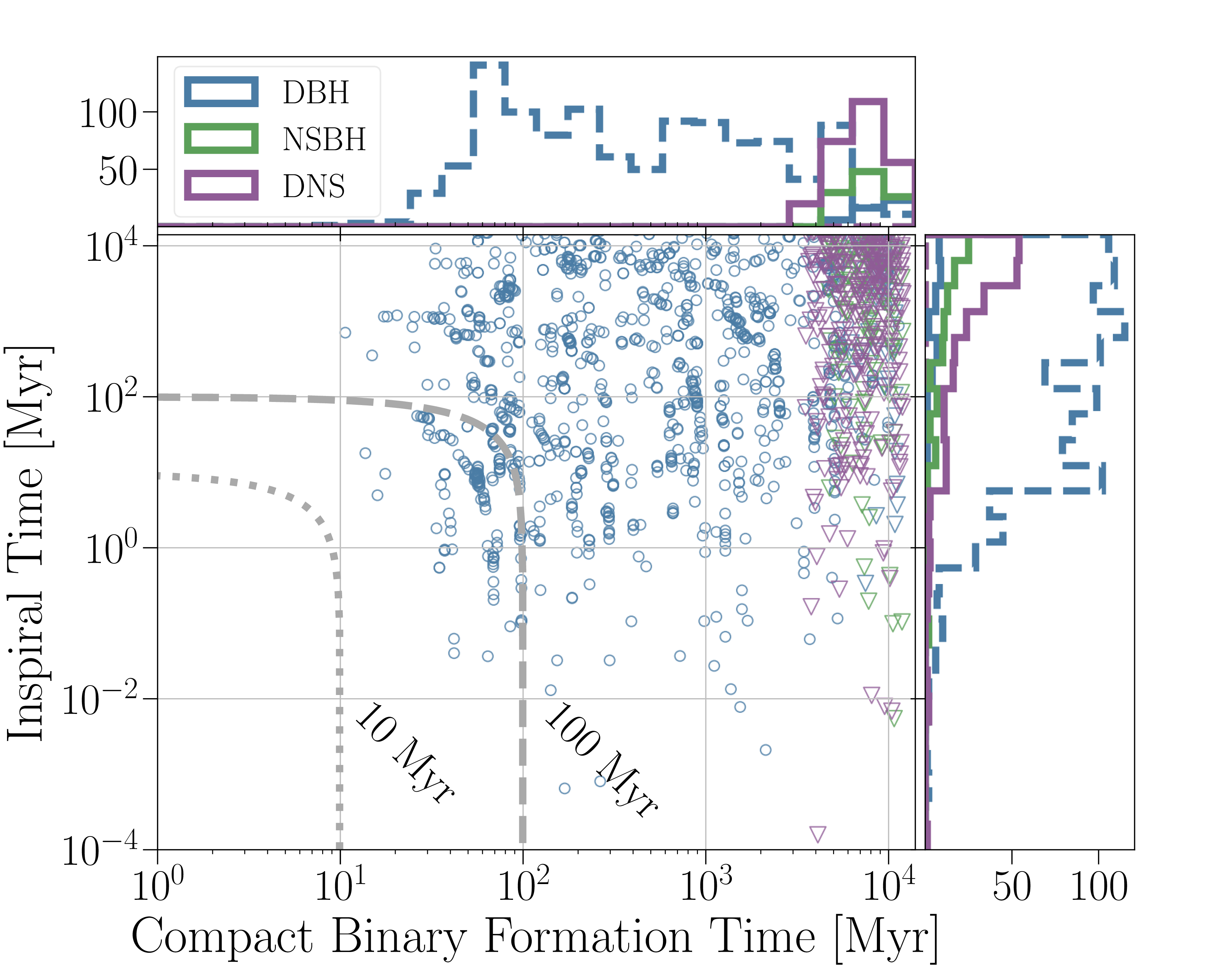


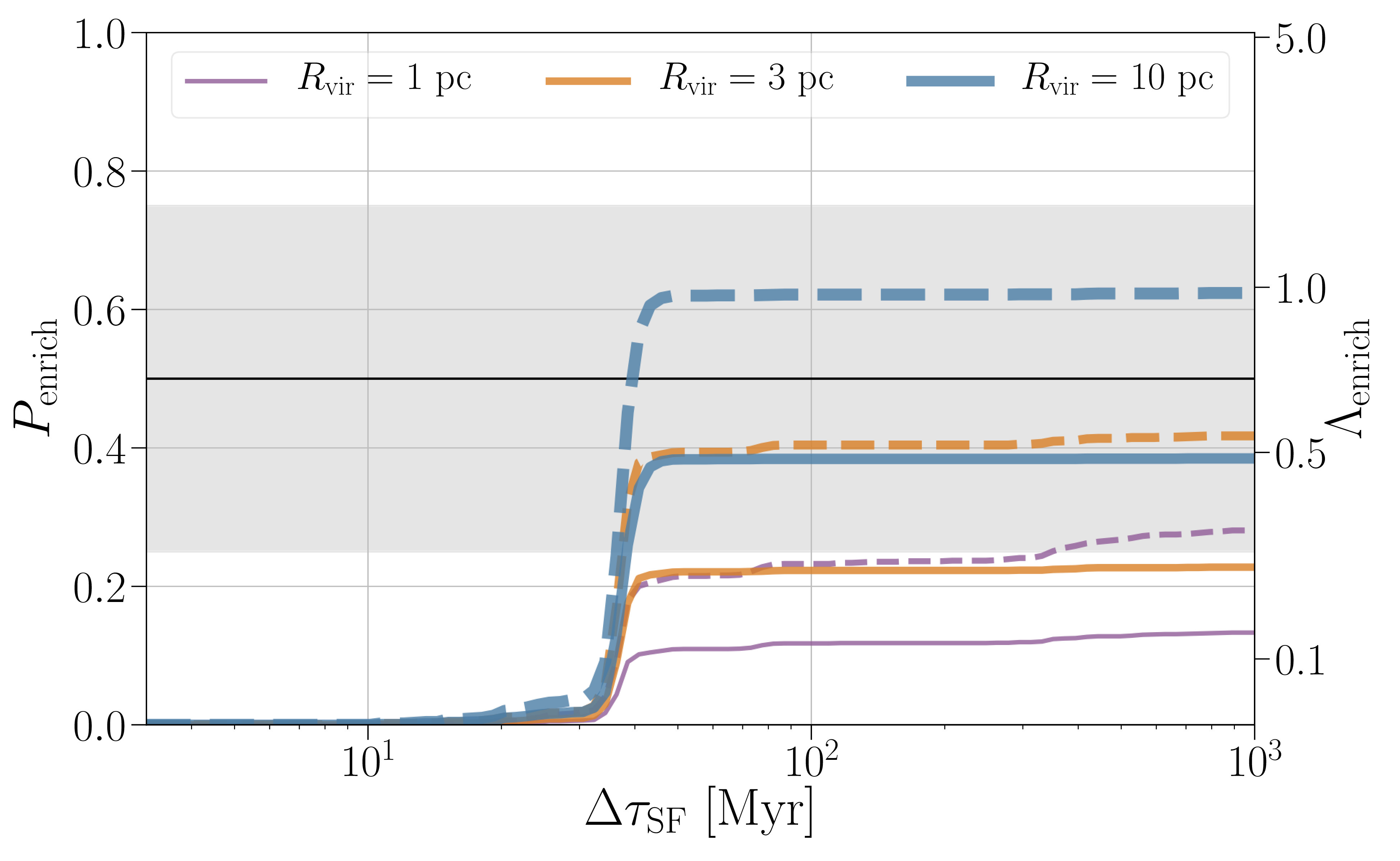


 solar masses (quoting the 90% range for parameters). This is larger than GW170817’s
  solar masses: we have a heavier binary.
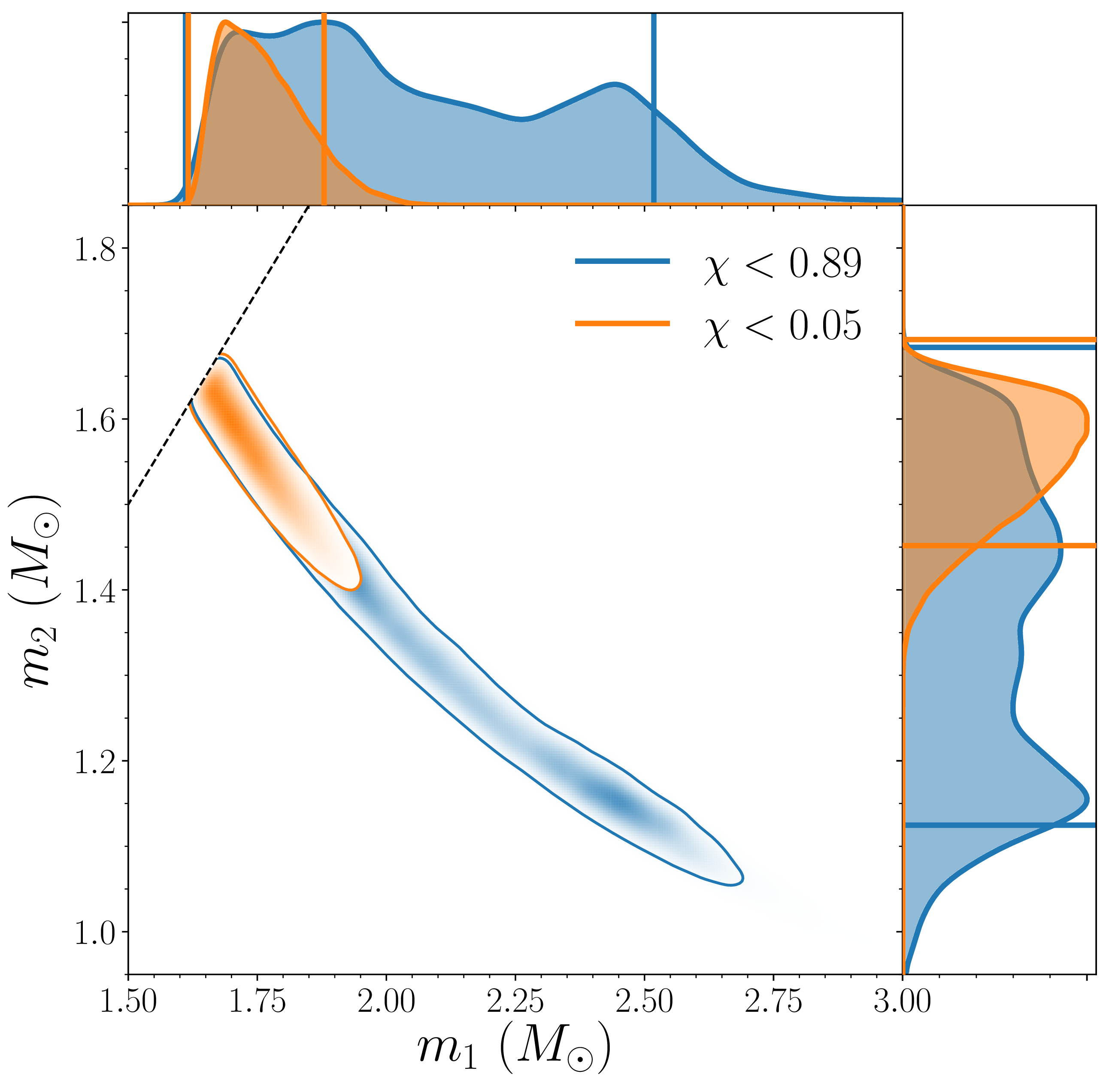
 –
– solar masses with the low-spin assumption, and
  –
– solar masses with the high-spin assumption; the lighter component has a mass
  –
– solar masses with the low-spin assumption, and
  –
– solar masses with the high-spin. These are the range of masses expected for neutron stars.
 . That means the signal was travelling across the Universe for about half a billion years. This is as many times bigger than diameter of Earth’s orbit about the Sun, as the diameter of the orbit is than the height of a LEGO brick. Space is big.
 –
–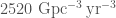 . Now, adding in the first 50 days of O3, we estimate the rate to be
  –
– , so roughly the same (which is nice) [
 , and the GW190425-like rate is lower at
  –
– . Combining the two (Assuming that binary neutron stars are all one class or the other), gives an overall rate of
  –
– , which is not too different than assuming the uniform distribution of masses.

 at a distance of
  (we typically quote results at the
  , much lower than for our binary black hole detections.
 –
– and
and  –
– . We have the convention that
  , which is why the masses look unequal; there’s a lot of support for them being nearly equal. These masses match what you’d expect for neutron stars.
 . This isn’t too informative, in terms of working out what neutron stars are made from, but we’ll come back to this in the
  and
and  , and that spins are below 0.4 (in between the limits used for parameter estimation). Given this, we infer that the merger rate is
  , safely within our previous upper limit [
 , adding in spatial coincidence too, and the probability becomes
  . It’s safe to conclude that the two are associated: merging binary neutron stars are the source of at least some short gamma-ray bursts!
 delay time between the inferred merger time and the gamma-ray burst. Given that signal has travelled for about 85 million years (taking the 5% lower limit on the inferred distance), this is a really small difference: gravity and light must travel at almost exactly the same speed. To derive exact limit you need to make some assumptions about when the gamma-rays were created. We’d expect some delay as it takes time for the jet to be created, and then for the gamma-rays to blast their way out of the surrounding material. We conservatively (and arbitrarily) take a window of the delay being 0 to 10 seconds, this gives
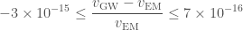 .
.
 , which we couldn’t test.
 . Considering the gravitational potential of the Milky Way, we find that
  [
[
 duration. The green line shows an approximate detection threshold for Fermi-GBM. Figure 4 from the
  (adding in the identification of the host galaxy, this becomes
  using the
  with the
 ,
, is the expansion velocity,
  is the Hubble constant and
  is the distance to the source. GW170817 is sufficiently nearby for this relationship to hold. We know the distance from the gravitational-wave measurement, and we can estimate the velocity from the redshift of the host galaxy. Therefore, it should be simple to combine the two to find the Hubble constant. Of course, there are a few complications…
 probability that AT 2017gfo would be as close to NGC 4993 on the sky by chance. Without a counterpart, it would still be possible to infer the Hubble constant statistically by cross-referencing the inferred gravitational-wave source location with the ensemble of compatible galaxies in a catalogue (you assign a probability to the source being associated with each galaxy, instead of saying it’s definitely in this one). The identification of NGC 4993 makes things much simpler.
 if we follow our
  .
. .
. (quoted as maximum a posteriori value and 68% interval, or
 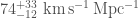 in the usual median-and-90%-interval convention). An updated set of results is given in the
  (68% interval using the low-spin prior). This is nicely (and diplomatically) consistent with existing results.
 –
– (assuming the low-spin mass results). These estimates can be feed into models for kilonovae to produce lightcurves, which we do. There is plenty of this type of modelling in the literature as observers try to understand their observations, so this is nothing special in terms of understanding this event. However, it could be useful in the future (once we have hoverboards), as we might be able to use gravitational-wave data to predict how bright a kilonova will be at different times, and so help astronomers decide upon their observing strategy.
 ). Together (i) and (ii) give the mass of r-process elements per binary neutron star (assuming that GW170817 is typical); (iii) and (iv) give total density of mergers throughout the history of the Universe, and combining everything together you get the total mass of r-process elements accumulated over time. Using the estimated binary neutron star merger rate of
 , and from binary neutron stars it is
  . There are on average
  binary black hole signals in detectors at a given time, and
  binary neutron star signals.


 to
to  range used for GW1708017. The middle and bottom rows assume a delay time of at least
  . Figure 5 of the
  , similar to what has been observed for
  (we assume that the star is just a helium core, with the outer hydrogen layers having been stripped off, hence the subscript); the pre-supernova orbital separation was
  , and the offset from the centre of the galaxy at the time of the supernova was
  . The main strongest constraints come from keeping the binary bound after the supernova; results are largely independent of the delay time once this gets above
  –
– ago from stars
  –
– and
and  –
– ).
).

 per flavour (
 in
in  window (top) about the GW170817 trigger time, and a
  window following GW170817 (bottom). IceCube is also sensitive to MeV neutrinos (none were detected). Fluences are the per-flavour sum of neutrino and antineutrino fluence, assuming equal fluence in all flavours. These are compared to theoretical predictions from
  to around
  (
( around the event and found nothing (
 of current sensitivity.
 ), we end up with a bigger, but still stable neutron star. Given our inferences from the inspiral (see the plot from the
  ), we have a supramassive neutron star. The rotation will slow down due to the emission of electromagnetic and gravitational radiation, and eventually the neutron star will collapse to a black hole. The time until collapse could take something like
 ), then we have a
 ), the merging neutron stars collapse down to a black hole.
 , too high for us to currently measure. However, if there is a neutron star, there may be slightly lower frequency gravitational waves from the neutron star matter wibbling about. We’re not exactly sure of the form of these signals, so we perform an unmodelled search for them (knowing the position of GW170817’s source helps for this).
 ) bursts. This searched a
  window including the merger time and covering the
  delay to the gamma-ray burst detection, and frequencies of
  –
– . Only LIGO data were used, as Virgo data suffered from large noise fluctuations above
  .
. ) bursts. This searched a
  –
– . This used LIGO and Virgo data.
 chunks), and frequencies
  . This used only LIGO data. There are two variations of STAMP: Zebragard and Lonetrack, and both are used here.
 for the four detectors, and search upper limits
  as a function of frequency. The noise amplitude spectral densities compare the sensitivities of the detectors. The search upper limits are root-sum-squared strain amplitudes at 50% detection efficiency. The colour code of the upper-limit markers indicates the search algorithm and the shape indicates the waveform injected to set the limits (the frequency is the average for this waveform). The bar mode waveform come from the rapid rotation of the supramassive neutron star leading to it becoming
  ! Go Virgo!
 for the high-spin prior and
  with the low-spin prior. The difference between the two results is because of the spin angular momentum slightly shifts the direction of the total angular momentum. Incorporating the distance information, for the high-spin prior the angle is
  (so the misalignment angle is
  ), and for the low-spin prior it is
  (misalignment
  ) [
) [
 . Parts of Figure 8 and 9 of the
  with the low-spin prior and
  with the high-spin prior. The difference is for the same reason as the difference in inclination measurements. The results are consistent with the distance to NGC 4993 [
 with the low-spin prior and
 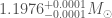 with the high-spin. This corresponds to a physical chirp mass of
  .
. , for the low-spin prior it is
  and for the high-spin prior it is
  .
. –
– and
and  –
–
 with the high-spin prior. Here, we quote maximum a posterior value and narrowest 68% intervals as opposed to the usual median and symmetric 90% credible interval. You might think its odd that the uncertainty is smaller when using the wider high-spin prior, but this is just another consequence of the difference in the inclination measurements. The values are largely in agreement with our initial values.
 . With the high-spin prior, we can only set an upper bound of
  . With the low-spin prior, we find that we are still consistent with zero deformation, but the distribution peaks away from zero. We have
  using the usual median and symmetric 90% credible interval, and
  if we take the narrowest 90% interval. This looks like we have detected matter effects, but since we’ve had to use the low-spin prior, which is only appropriate for neutron stars, this would be a circular argument. More details on what we can learn about tidal deformations and what neutron stars are made of, under the assumption that we do have neutron stars, are given in the
  of the coalescence time). We still don’t find anything, but now we set much tighter upper limits on what signal there could be there.
 ), as well as it being thermodynamically stable. Accommodating the most massive neutron star turns out to be an important piece of information.
 neutron star, these results indicate that the tidal deformation parameter would be
  . We favour softer equations of state over stiffer ones [
 must be greater than that for the smaller neutron star
  . The green shading and (50% and 90%) contours are calculated using the equation-of-state insensitive relations. The blue contours are for the parametrised equation-of-state model. The orange contours are from the
  ) neutron star is
  and the radius of the lighter (
 –
– ) neutron star is
  . With the parametrised equation-of-state model, the radii are
  (
( ) and
) and  (
( –
–
 in radius. We now know that’s not the case.
 , which is basically all (99.996%) of them. Therefore, it’s unlikely that a cluster is the source of this binary.
 (3-sigma upper limit of
  ), towards the bottom end of our range, but their rate increases if not all mergers are as bright as AT 2017gfo.
 . They use to estimate the probability that AT 2017gfo and GW170817 are just a chance coincidence and are actually unrelated. The probability is
  at 90% confidence.
 , safely above our range.
 and
and  . Their figure 3 shows that this is well above expected rates.
 . That’s not too bad, but do stick with our result.
 ): LSST and WFIRST will see lots, about 7 and 8 per year respectively.
 . They project that around 30% of gravitational-wave detections will be accompanied by gamma-ray bursts, once LIGO and Virgo reach design sensitivity.
 . To match up to our binary neutron star merger rate, we either need only a fraction of binary neutron star mergers to produce kilonova or for them to only be observable for viewing angles of less than
  . Their table 2 contains a nice compilation of rates for short gamma-ray bursts.

 after 67 days post-merger, but this evolves little over the duration of their observations (to day 152 post-merger), also suggesting a turn-over.
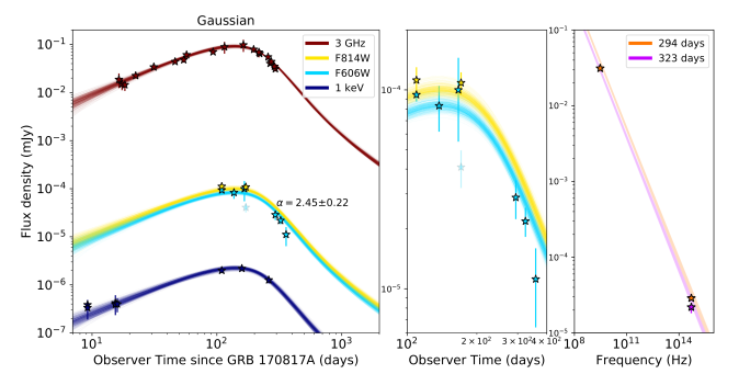
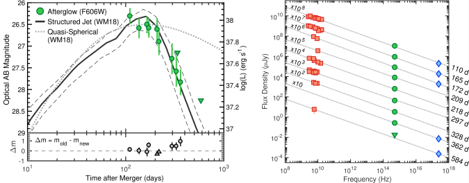


 .
. of the line of sight, and derive
  .
. using the Milky Way’s potential and
  using the Virgo cluster’s potential.
 , and that we are viewing it at an angle of
  . With X-ray and radio observations to 359 days,
  , and the width of a Gaussian structured jet would be
  . Using a combination of gravitational-wave, optical, radio and X-ray data,
  , for a Gaussian structured jet where they estimates the width
  . Using broadband synchrotron data to 800 days with a boosted fireball model,
  .
. , which (unsurprisingly) agrees pretty well with the result we obtained using the
  (where the errors are statistical uncertainty and an estimate of systematic error from calibration of the strain).
 (quoting median and 68% symmetric credible interval). Using different jet models changes their value for the Hubble constant a little; the choice of spin prior does not (since we get basically all of the inclination information from their radio observations). The results is still consistent with Planck and SH0ES, but is closer to the Planck value.
 . Combining this with results from the
  .
. , and hence
  .
. and a dark matter halo mass of
  , where we use the
  (but conclusions are similar using the
  . They also look at the star formation history, 90% were formed by
  ago, and the median mass-weighted stellar age is
  . From this they infer a merger delay time of
  −
− . From this, and assuming that the system was born close to its current location, they estimate that the supernova kick
  , towards the lower end of our estimate. They use
  .
. −
− and the mean stellar age is greater than about
  . They also give a luminosity distance estimate of
  , which overlaps with our gravitational-wave estimate. I’m not sure what value of
  they are using.
 . They find that 60% of stars by mass are older than
  and that less than 1% are less than
  old. Their Figure 5 has some information on likely supernova kicks, they conclude it was probably small, but don’t quantify this. They use
  .
. . They calculate a mass-weighted mean stellar age of
  and a likely minimum age for GW170817’s source system of
  . They use
  .
. , and suggest an old stellar population of age
  .
. and find a halo mass of
 and
and  ago.
ago. .
. . This implies a value for the Hubble constant of
  .
. . A neutron star would irradiate the ejecta with neutrinos, lower the neutron fraction and making the ejecta bluer. Since it is red, the neutrino flux must have been shut off, and the neutron star must have collapsed. We are in case b in their figure below.
 ). This is difficult to resolve unless neutron star radii are small (
 ).
).  –
– .
.  .
. has a radius of at least
  . They also estimate that the radius for the maximum mass nonrotating neutron star must be greater than
  .
.  , and for
  is greater than
  .
. ). They argue that the latter condition implies that the radius of a
  and the former that it is less than
  .
. . This is consistent with results in the
  .
. .
.
 inferred by


 –
– , whereas most of the radii inferred for GW170817’s components are larger. This paper argues that this can be resolved if one of the components of GW170817’s source was a hadron–quark hybrid star or a quark star.
 , which I think makes this an OK approximation;
  –
– .
. –
– and the radius in the range
  –
– .
. . These results are in good agreement with ours, their inclusion of electromagnetic data pushes their combined results towards larger values for the tidal deformation.
 –
– and the neutron star radius is
  –
– .
. .
. .
. (about 3%).
 .
.


 ). The lower panel shows how we removed the glitch: the grey line shows


 is the component of the spin aligned with the orbital angular momentum. The two-dimensional shows the 90% probability contour, which follows a line of constant chirp mass. The one-dimensional plot shows individual masses; the dotted lines mark 90% bounds away from equal mass. Figure 4 of the
  .
.
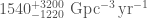 (assuming a uniform of neutron star masses between one and two solar masses). This is surprisingly close to what the Collaboration expected back in
  and
and  , with a realistic rate of
 .
.
 is the merger rate, and
  is the surveyed time–volume (you expect more detections if your detectors are more sensitive, so that they can find signals from further away, or if you leave them on for longer). We can estimate
  . We use a uniform prior, for consistency with what we’ve done in the past.
 confidence level limit on the rate is
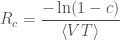 ,
,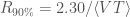
 , the equivalent results is
![\displaystyle R_c = \frac{\left[\mathrm{erf}^{-1}(c)\right]^2}{\langle VT \rangle}](https://s0.wp.com/latex.php?latex=%5Cdisplaystyle+R_c+%3D+%5Cfrac%7B%5Cleft%5B%5Cmathrm%7Berf%7D%5E%7B-1%7D%28c%29%5Cright%5D%5E2%7D%7B%5Clangle+VT+%5Crangle%7D&bg=ffffff&fg=444444&s=0&c=20201002) ,
, , so results would be the same to within a factor of 2, but the results with the uniform prior are more conservative.
 for isotropic spins up to 0.05, and
  if you allow the spins up to 0.4.
 to
to  for a 1.4 solar mass neutron star and a black hole between 30 and 5 solar masses and a range of different spins (Table II of the
 and if they all come from neutron star–black hole mergers the angle needs to be bigger than
  .
.
 , and define an effective distance
  defined so that
  where
where  is the analysed amount of time. The plot below show our limits on rate and effective distance for our different injections.
 indicates the spin aligned with the orbital angular momentum. Figure 2 of the

 , the mass ratio
  and the total mass
  , where
  and
and  are the masses of the primary and secondary neutron stars respectively. The uncertainties are small for louder signals (higher signal-to-noise ratio). If we neglect the spin, the true chirp mass can lie outside the posterior distribution, the average is about 5 standard deviations from the mean, but if we include spin, the offset is just 0.7 from the mean (there’s still some offset as we’re allowing for spins all the way up to 1).


 , where
  is the 90% sky area and
  is the signal-to-noise ratio. The results for BAYESTAR and LALInference agree, as do the results with Gaussian and recoloured noise. This is Figure 9 of Berry et al. (
 .
. . We can get this from less dominant parts of the waveform, but it’s not typically measured as precisely as the chirp mass, so we’re often left with big uncertainties.