Gravity Spy is an awesome project that combines citizen science and machine learning to classify glitches in LIGO and Virgo data. Glitches are short bursts of noise in our detectors which make analysing our data more difficult. Some glitches have known causes, others are more mysterious. Classifying glitches into different types helps us better understand their properties, and in some cases track down their causes and eliminate them! In this paper, led by Scotty Coughlin, we demonstrated the effectiveness of a new tool which are citizen scientists can use to identify new glitch classes.
The Gravity Spy project
Gravitational-wave detectors are complicated machines. It takes a lot of engineering to achieve the required accuracy needed to observe gravitational waves. Most of the time, our detectors perform well. The background noise in our detectors is easy to understand and model. However, our detectors are also subject to glitches, unusual (sometimes extremely loud and complicated) noise that doesn’t fit the usual properties of noise. Glitches are short, they only appear in a small fraction of the total data, but they are common. This makes detection and analysis of gravitational-wave signals more difficult. Detection is tricky because you need to be careful to distinguish glitches from signals (and possibly glitches and signals together), and understanding the signal is complicated as we may need to model a signal and a glitch together [bonus note]. Understanding glitches is essential if gravitational-wave astronomy is to be a success.
To understand glitches, we need to be able to classify them. We can search for glitches by looking for loud pops, whooshes and splats in our data. The task is then to spot similarities between them. Once we have a set of glitches of the same type, we can examine the state of the instruments at these times. In the best cases, we can identify the cause, and then work to improve the detectors so that this no longer happens. Other times, we might be able to find the source, but we can find one of the monitors in our detectors which acts a witness to the glitch. Then we know that if something appears in that monitor, we expect a glitch of a particular form. This might mean that we throw away that bit of data, or perhaps we can use the witness data to subtract out the glitch. Since glitches are so common, classifying them is a huge amount of work. It is too much for our detector characterisation experts to do by hand.
There are two cunning options for classifying large numbers of glitches
- Get a computer to do it. The difficulty is teaching a computer to identify the different classes. Machine-learning algorithms can do this, if they are properly trained. Training can require a large training set, and careful validation, so the process is still labour intensive.
- Get lots of people to help. The difficulty here is getting non-experts up-to-speed on what to look for, and then checking that they are doing a good job. Crowdsourcing classifications is something citizen scientists can do, but we will need a large number of dedicated volunteers to tackle the full set of data.
The idea behind Gravity Spy is to combine the two approaches. We start with a small training set from our detector characterization experts, and train a machine-learning algorithm on them. We then ask citizen scientists (thanks Zooniverse) to classify the glitches. We start them off with glitches the machine-learning algorithm is confident in its classification; these should be easy to identify. As citizen scientists get more experienced, they level up and start tackling more difficult glitches. The citizen scientists validate the classifications of the machine-learning algorithm, and provide a larger training set (especially helpful for the rarer glitch classes) for it. We can then happily apply the machine-learning algorithm to classify the full data set [bonus note].

How Gravity Spy works: the interconnection of machine-learning classification and citizen-scientist classification. The similarity search is used to identify glitches similar to one which do not fit into current classes. Figure 2 of Coughlin et al. (2019).
I especially like the levelling-up system in Gravity Spy. I think it helps keep citizen scientists motivated, as it both prevents them from being overwhelmed when they start and helps them see their own progress. I am currently Level 4.
Gravity Spy works using images of the data. We show spectrograms, plots of how loud the output of the detectors are at different frequencies at different times. A gravitational wave form a binary would show a chirp structure, starting at lower frequencies and sweeping up.
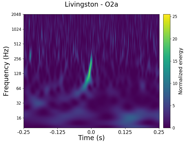
Spectrogram showing the upward-sweeping chirp of gravitational wave GW170104 as seen in Gravity Spy. I correctly classified this as a Chirp.
New glitches
The Gravity Spy system works smoothly. However, it is set up to work with a fixed set of glitch classes. We may be missing new glitch classes, either because they are rare, and hadn’t been spotted by our detector characterization team, or because we changed something in our detectors and new class arose (we expect this to happen as we tune up the detectors between observing runs). We can add more classes to our citizen scientists and machine-learning algorithm to use, but how do we spot new classes in the first place?
Our citizen scientists managed to identify a few new glitches by spotting things which didn’t fit into any of the classes. These get put in the None-of-the-Above class. Occasionally, you’ll come across similar looking glitches, and by collecting a few of these together, build a new class. The Paired Dove and Helix classes were identified early on by our citizen scientists this way; my favourite suggested new class is the Falcon [bonus note]. The difficulty is finding a large number of examples of a new class—you might only recognise a common feature after going past a few examples, backtracking to find the previous examples is hard, and you just have to keep working until you are lucky enough to be given more of the same.

Example Helix (left) and Paired Dove glitches. These classes were identified by Gravity Spy citizen scientists. Helix glitches are related to related to hiccups in the auxiliary lasers used to calibrate the detectors by pushing on the mirrors. Paired Dove glitches are related to motion of the beamsplitter in the interferometer. Adapted from Figure 8 of Zevin et al. (2017).
To help our citizen scientists find new glitches, we created a similar search. Having found an interesting glitch, you can search for similar examples, and put quickly put together a collection of your new class. The video below shows how it works. The thing we had to work out was how to define similar?
Transfer learning
Our machine-learning algorithm only knows about the classes we tell it about. It then works out the features we distinguish the different classes, and are common to glitches of the same class. Working in this feature space, glitches form clusters of different classes.

Visualisation showing the clustering of different glitches in the Gravity Spy feature space. Each point is a different glitch from our training set. The feature space has more than three dimensions: this visualisation was made using a technique which preserves the separation and clustering of different and similar points. Figure 1 of Coughlin et al. (2019).
For our similarity search, our idea was to measure distances in feature space [bonus note for experts]. This should work well if our current set of classes have a wide enough set of features to capture to characteristics of the new class; however, it won’t be effective if the new class is completely different, so that its unique features are not recognised. As an analogy, imagine that you had an algorithm which classified M&M’s by colour. It would probably do well if you asked it to distinguish a new colour, but would probably do poorly if you asked it to distinguish peanut butter filled M&M’s as they are identified by flavour, which is not a feature it knows about. The strategy of using what a machine learning algorithm learnt about one problem to tackle a new problem is known as transfer learning, and we found this strategy worked well for our similarity search.
Raven Pecks and Water Jets
To test our similarity search, we applied it to two glitches classes not in the Gravity Spy set:
- Raven Peck glitches are caused by thirsty ravens pecking ice built up along nitrogen vent lines outside of the Hanford detector. Raven Pecks look like horizontal lines in spectrograms, similar to other Gravity Spy glitch classes (like the Power Line, Low Frequency Line and 1080 Line). The similarity search should therefore do a good job, as we should be able to recognise its important features.
- Water Jet glitches were caused by local seismic noise at the Hanford detector which causes loud bands which disturb the input laser optics. These glitches are found between , over which time there are 26,871 total glitches in GRavity Spy. The Water Jet glitch doesn’t have anything to do with water, it is named based on its appearance (like a fountain, not a weasel). Its features are subtle, and unlike other classes, so we would expect this to be difficult for our similarity search to handle.
These glitches appeared in the data from the second observing run. Raven Pecks appeared between 14 April and 9 August 2017, and Water Jets appeared 4 January and 28 May 2017. Over these intervals there are a total of 13,513 and 26,871 Gravity Spy glitches from all type, so even if you knew exactly when to look, you have a large number to search through to find examples.
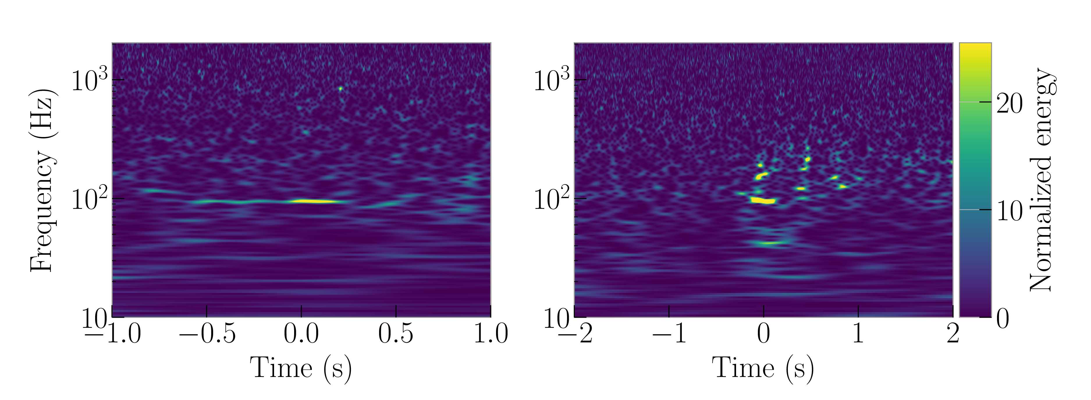
Example Raven Peck (left) and Water Jet (right) glitches. These classes of glitch are not included in the usual Gravity Spy scheme. Adapted from Figure 3 of Coughlin et al. (2019).
We tested using our machine-learning feature space for the similarity search against simpler approaches: using the raw difference in pixels, and using a principal component analysis to create a feature space. Results are shown in the plots below. These show the fraction of glitches we want returned by the similarity search versus the total number of glitches rejected. Ideally, we would want to reject all the glitches except the ones we want, so the search would return 100% of the wanted classes and reject almost 100% of the total set. However, the actual results will depend on the adopted threshold for the similarity search: if we’re very strict we’ll reject pretty much everything, and only get the most similar glitches of the class we want, if we are too accepting, we get everything back, regardless of class. The plots can be read as increasing the range of the similarity search (becoming less strict) as you go left to right.
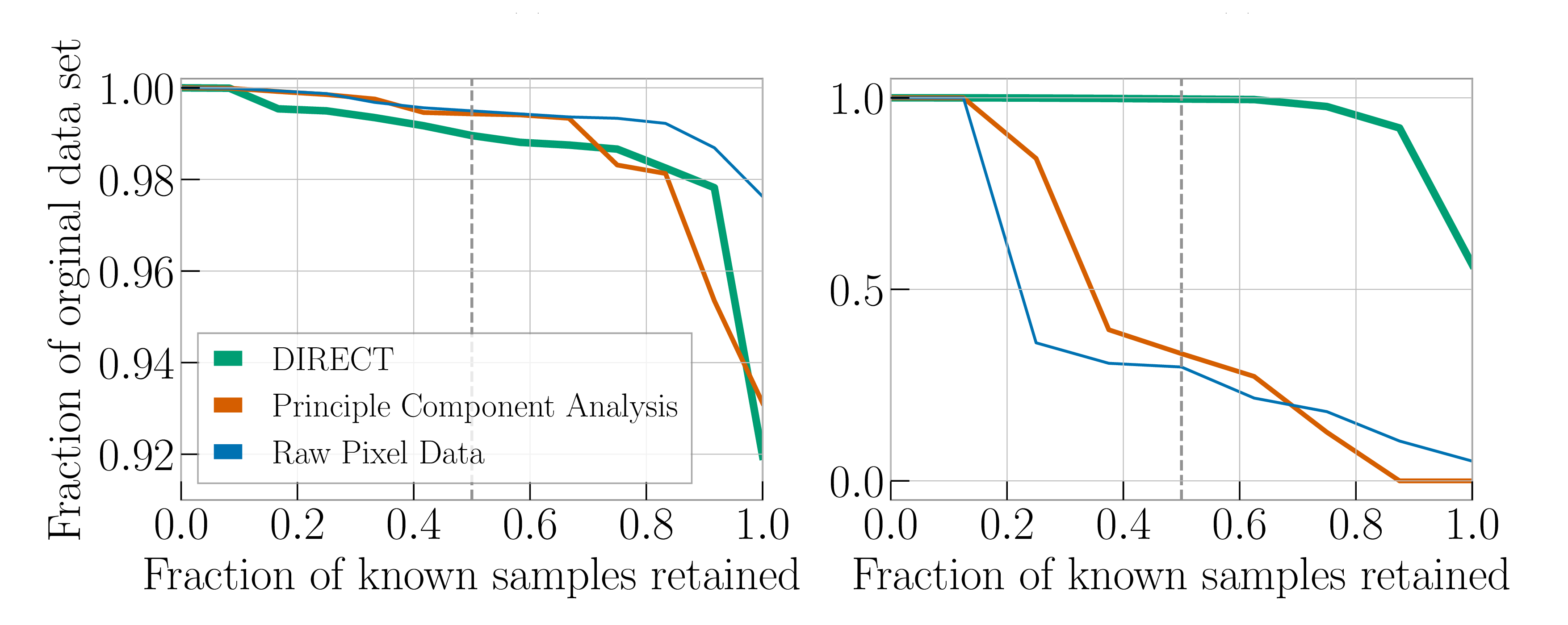
Performance of the similarity search for Raven Peck (left) and Water Jet (right) glitches: the fraction of known glitches of the desired class that have a higher similarity score (compared to an example of that glitch class) than a given percentage of full data set. Results are shown for three different ways of defining similarity: the DIRECT machine-learning algorithm feature space (think line), a principal component analysis (medium line) and a comparison of pixels (thin line). Adapted from Figure 3 of Coughlin et al. (2019).
For the Raven Peck, the similarity search always performs well. We have 50% of Raven Pecks returned while rejecting 99% of the total set of glitches, and we can get the full set while rejecting 92% of the total set! The performance is pretty similar between the different ways of defining feature space. Raven Pecks are easy to spot.
Water Jets are more difficult. When we have 50% of Water Jets returned by the search, our machine-learning feature space can still reject almost all glitches. The simpler approaches do much worse, and will only reject about 30% of the full data set. To get the full set of Water Jets we would need to loosen the similarity search so that it only rejects 55% of the full set using our machine-learning feature space; for the simpler approaches we’d basically get the full set of glitches back. They do not do a good job at narrowing down the hunt for glitches. Despite our suspicion that our machine-learning approach would struggle, it still seems to do a decent job [bonus note for experts].
Do try this at home
Having developed and testing our similarity search tool, it is now live. Citizen scientists can use it to hunt down new glitch classes. Several new glitches classes have been identified in data from LIGO and Virgo’s (currently ongoing) third observing run. If you are looking for a new project, why not give it a go yourself? (Or get your students to give it a go, I’ve had some reasonable results with high-schoolers). There is the real possibility that your work could help us with the next big gravitational-wave discovery.
arXiv: arXiv:1903.04058 [astro-ph.IM]
Journal: Physical Review D; 99(8):082002(8); 2019
Websites: Gravity Spy; Gravity Spy Tools
Gravity Spy blog: Introducing Gravity Spy Tools
Current stats: Gravity Spy has 15,500 registered users, who have made 4.4 million glitch classifications, leading to 200,000 successfully identified glitches.
Bonus notes
Signals and glitches
The best example of a gravitational-wave overlapping a glitch is GW170817. The glitch meant that the signal in the LIGO Livingston detector wasn’t immediately recognised. Fortunately, the signal in the Hanford detector was easy to spot. The glitch was analyse and categorised in Gravity Spy. It is a simple glitch, so it wasn’t too difficult to remove from the data. As our detectors become more sensitive, so that detections become more frequent, we expect that signal overlapping with glitches will become a more common occurrence. Unless we can eliminate glitches, it is only a matter of time before we get a glitch that prevents us from analysing an important signal.
Gravitational-wave alerts
In the third observing run of LIGO and Virgo, we send out automated alerts when we have a new gravitational-wave candidate. Astronomers can then pounce into action to see if they can spot anything coinciding with the source. It is important to quickly check the state of the instruments to ensure we don’t have a false alarm. To help with this, a data quality report is automatically prepared, containing many diagnostics. The classification from the Gravity Spy algorithm is one of many pieces of information included. It is the one I check first.
The Falcon
Excellent Gravity Spy moderator EcceruElme suggested a new glitch class Falcon. This suggestion was followed up by Oli Patane, they found that all the examples identified occured between 6:30 am and 8:30 am on 20 June 2017 in the Hanford detector. The instrument was misbehaving at the time. To solve this, the detector was taken out of observing mode and relocked (the equivalent of switching it off and on again). Since this glitch class was only found in this one 2-hour window, we’ve not added it as a class. I love how it was possible to identify this problematic stretch of time using only Gravity Spy images (which don’t identify when they are from). I think this could be the seed of a good detective story. The Hanfordese Falcon?
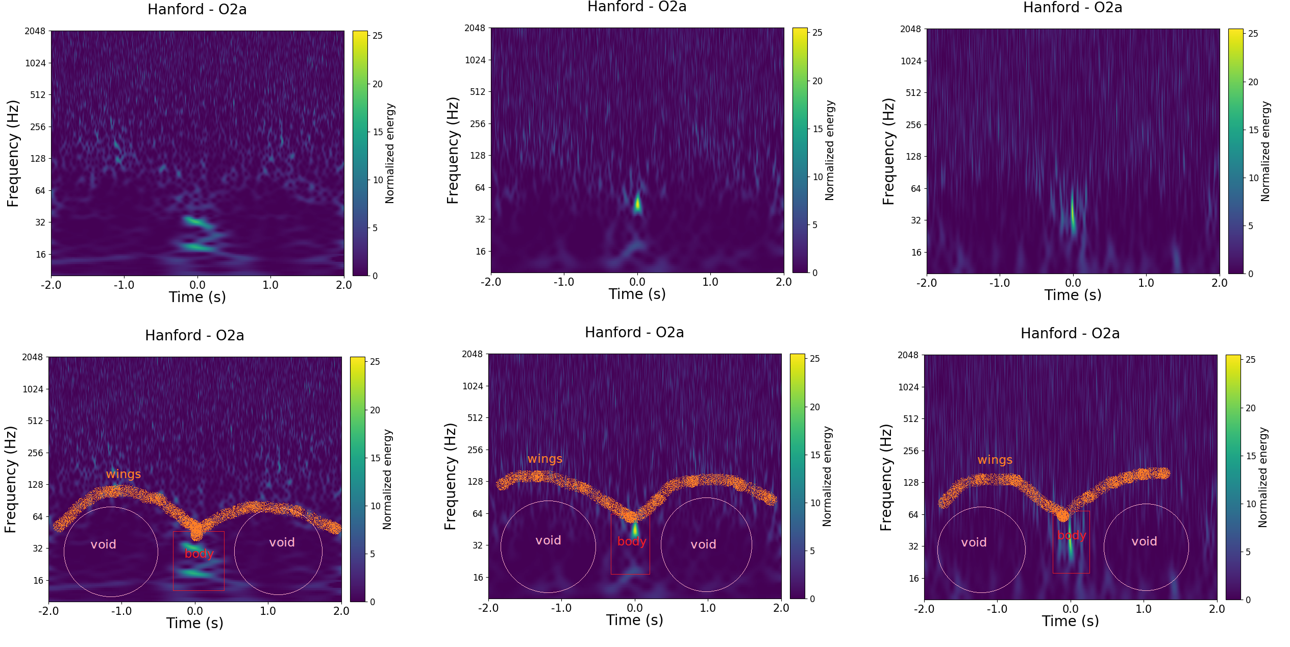
Examples of the proposed Falcon glitch class, illustrating the key features (and where the name comes from). This new glitch class was suggested by Gravity Spy citizen scientist EcceruElme.
Distance measure
We chose a cosine distance to measure similarity in feature space. We found this worked better than a Euclidean metric. Possibly because for identifying classes it is more important to have the right mix of features, rather than how significant the individual features are. However, we didn’t do a systematic investigation of the optimal means of measuring similarity.
Retraining the neural net
We tested the performance of the machine-learning feature space in the similarity search after modifying properties of our machine-learning algorithm. The algorithm we are using is a deep multiview convolution neural net. We switched the activation function in the fully connected layer of the net, trying tanh and leaukyREU. We also varied the number of training rounds and the number of pairs of similar and dissimilar images that are drawn from the training set each round. We found that there was little variation in results. We found that leakyREU performed a little better than tanh, possibly because it covers a larger dynamic range, and so can allow for cleaner separation of similar and dissimilar features. The number of training rounds and pairs makes negligible difference, possibly because the classes are sufficiently distinct that you don’t need many inputs to identify the basic features to tell them apart. Overall, our results appear robust. The machine-learning approach works well for the similarity search.
 –
– , which is about
  –
–
 –
– galaxies.


 is inversely proportional to the sixth power of the signal-to-noise ration
  . This is what you would expect. The localization volume depends upon the angular uncertainty on the sky
  , the distance to the source
  , and the distance uncertainty
  ,
, .
. .
. .
. .
.