Chris Moore

April was a busy month. Amongst other adventures, I organised the 15th British Gravity (BritGrav) Meeting. This is a conference for everyone involved with research connected to gravitation. I was involved in organising last year’s meeting in Cambridge, and since there were very few fatalities, it was decided that I could be trusted to organise it again. Overall, I think it actually went rather well.

Before I go on to review the details of the meeting, I must thank everyone who helped put things together. Huge thanks to my organisational team who helped with every aspect of the organisation. They did wonderfully, even if Hannah seems to have developed a slight sign-making addiction. Thanks go to Classical & Quantum Gravity and the IOP Gravitational Physics Group for sponsoring the event, and to the College of Engineering & Physical Sciences’ marketing team for advertising. Finally, thanks to everyone who came along!

Talks

BritGrav is a broad meeting. It turns out there’s rather a lot of research connected to gravity! This has both good and bad aspects. On the plus side, you can make connections with people you wouldn’t normally run across and find out about new areas you wouldn’t hear about at a specialist meeting. On the negative side, there can some talks which go straight-over your head (no matter how fast your reaction are). The 10-minute talk format helps a little here. There’s not enough time to delve into details (which only specialists would appreciate) so speakers should stick to giving an overview that is generally accessible. Even in the event that you do get completely lost, it’s only a few minutes until the next talk, so it’s not too painful. The 10-minute time slot also helps us to fit in a large number of talks, to cover all the relevant areas of research.

Slide from Teodora Oniga’s BritGrav 15 talk on gauge invariant quantum gravitational decoherence. There are not enough cats featured in slides on gravitational physics.

I’ve collected together tweets and links from the science talks: it was a busy two days! We started with Chris Collins talking about testing the inverse-square law here at Birmingham. There were a couple more experimental talks leading into a session on gravitational waves, which I enjoyed particularly. I spoke on a soon-to-be published paper, and Birmingham PhDs Hannah Middleton and Simon Stevenson gave interesting talks on what we could learn about black holes from gravitational waves.

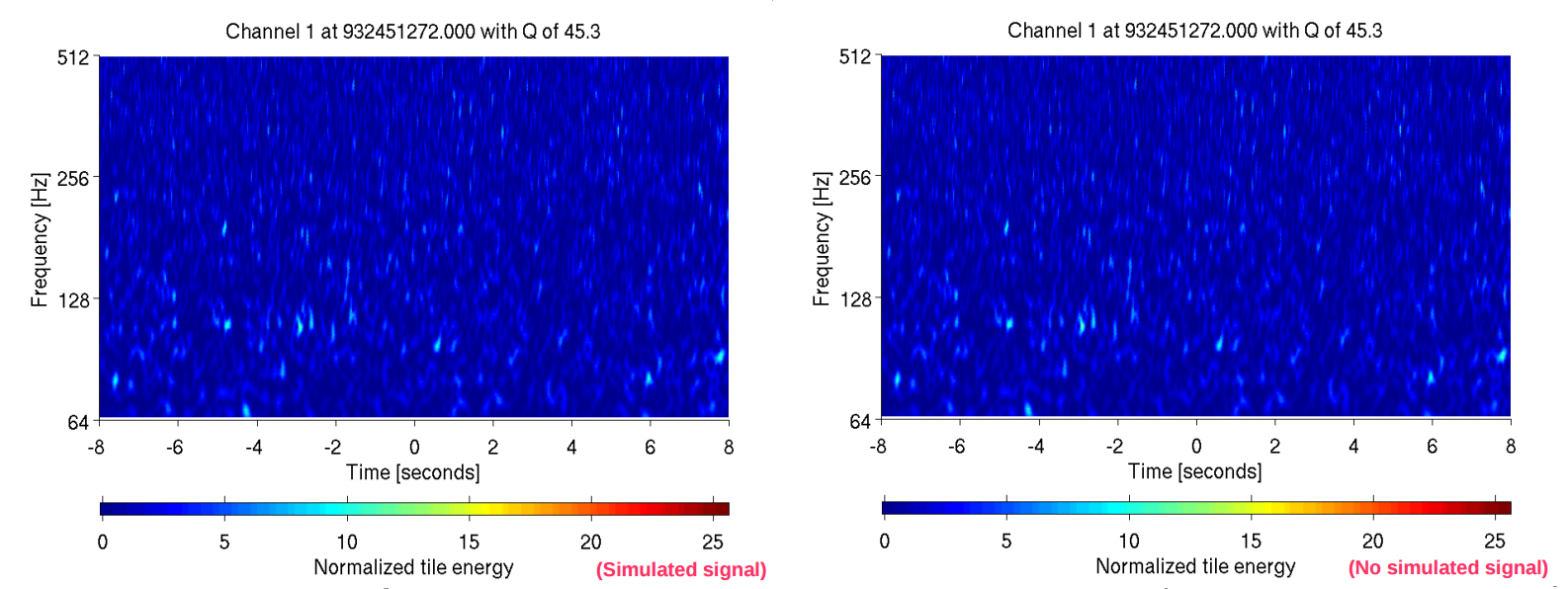
Detecting neutron star–black hole binaries

Slides demonstrating the difficulty of detecting gravitational-wave signals from Alex Nielsen’s talk on searching for neutron star–black hole binaries with gravitational waves. Fortunately we don’t do it by eye (although if you flick between the slides you can notice the difference).

In the afternoon, there were some talks on cosmology (including a nice talk from Maggie Lieu on hierarchical modelling) and on the structure of neutron stars. I was especially pleased to see a talk by Alice Harpole, as she had been one of my students at Cambridge (she was always rather good). The day concluded with some numerical relativity and the latest work generating gravitational-waveform templates (more on that later).

The second day was more theoretical, and somewhat more difficult for me. We had talks on modified gravity and on quantum theories. We had talks on the properties of various spacetimes. Brien Nolan told us that everyone should have a favourite spacetime before going into the details of his: McVittie. That’s not the spacetime around a biscuit, sadly, but could describe a black hole in an expanding Universe, which is almost as cool.

The final talks of the day were from the winners of the Gravitational Physics Group’s Thesis Prize. Anna Heffernan (2014 winner) spoke on the self-force problem. This is important for extreme-mass-ratio systems, such as those we’ll hopefully detect with eLISA. Patricia Schmidt (2105 winner) spoke on including precession in binary black hole waveforms. In general, the spins of black holes won’t be aligned with their orbital angular momentum, causing them to precess. The precession modulates the gravitational waveform, so you need to include this when analysing signals (especially if you want to measure the black holes’ spins). Both talks were excellent and showed how much work had gone into the respective theses.

The meeting closed with the awarding of the best student-talk prize, kindly sponsored by Classical & Quantum Gravity. Runners up were Viraj Sanghai and Umberto Lupo. The winner was Christopher Moore from Cambridge. Chris gave a great talk on how to include uncertainty about your gravitational waveform (which is important if you don’t have all the physics, like precession, accurately included) into your parameter estimation: if your waveform is wrong, you’ll get the wrong answer. We’re currently working on building waveform uncertainty into our parameter-estimation code. Chris showed how you can think about this theoretical uncertainty as another source of noise (in a certain limit).

There was one final talk of the day: Jim Hough gave a public lecture on gravitational-wave detection. I especially enjoyed Jim’s explanation that we need to study gravitational waves to be prepared for the 24th century, and hearing how Joe Weber almost got into a fist fight arguing about his detectors (hopefully we’ll avoid that with LIGO). I hope this talk enthused our audience for the first observations of Advanced LIGO later this year: there were many good questions from the audience and there was considerable interest in our table-top Michelson interferometer afterwards. We had 114 people in the audience (one of the better turn outs for recent outreach activities), which I was delighted with.

Attendance

We had a fair amount of interest in the meeting. We totalled 81 (registered) participants at the meeting: a few more registered but didn’t make it in the end for various reasons and I suspect a couple of Birmingham people sneaked in without registering.

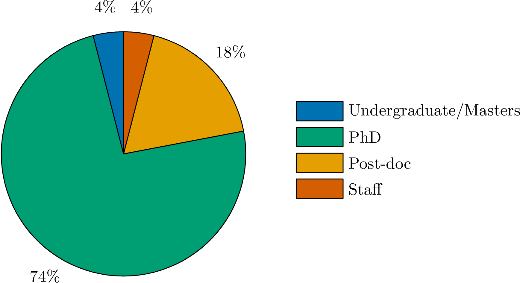
Looking at the attendance in more detail, we can break down the participants by their career-level. One of the aims of BritGrav is to showcase to research of early-career researchers (PhD students and post-docs), so we ask for this information on the registration form. The proportions are shown in the pie-chart below.

Attendance at BritGrav 15 by career level

Proportion of participants at BritGrav 15 by (self-reported) career level.

PhD students make up the largest chunk; there are a few keen individuals who are yet to start a PhD, and a roughly even split between post-docs and permanent staff. We do need to encourage more senior researchers to come along, even if they are not giving talks, so that they can see the research done by others.

We had a total of 50 talks across the two days (including the two thesis-prize talks); the distribution of talks by career level as shown below.

Proportion of talks at BritGrav 15 by (self-reported) career level. The majority are by PhD students.

PhDs make up an even larger proportion of talks here, and we see that there are many more talks from post-docs than permanent staff members. This is exactly what we’re aiming for! For comparison, at the first BritGrav Meeting only 26% of talks were by PhD students, and 17% of talks were by post-docs. There’s been a radical change in the distribution of talks, shifting from senior to junior, although the contribution by post-docs ends up about the same.

We can also consider at the proportion of participants from different institutions, which is shown below.

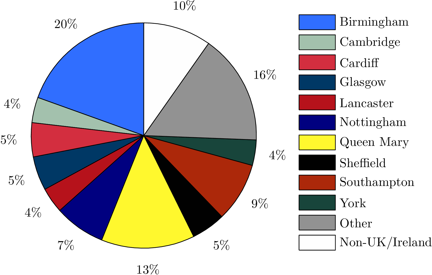
Attendance at BritGrav 15 by institution

Proportion of participants at BritGrav 15 by institution. Birmingham, as host, comes out top.

Here, any UK/Ireland institution which has one or no speakers is lumped together under “Other”, all these institutions had fewer than four participants. It’s good to see that we are attracting some international participants: of those from non-UK/Ireland institutions, two are from the USA and the rest are from Europe (France, Germany, The Netherlands and Slovenia). Birmingham makes up the largest chunk, which probably reflects the convenience. The list of top institutions closely resembles the list of institutions that have hosted a BritGrav. This could show that these are THE places for gravitational research in the UK, or possibly that the best advertising for future BritGravs is having been at an institution in the past (so everyone knows how awesome they are). The distribution of talks by institution roughly traces the number of participants, as shown below.

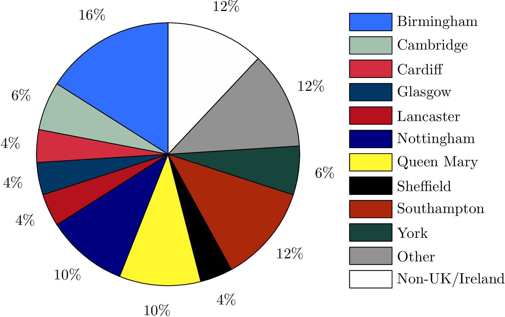
Proportion of talks at BritGrav 15 by institution.

Again Birmingham comes top, followed by Queen Mary and Southampton. Both of the thesis-prize talks were from people currently outside the UK/Ireland, even though they studied for their PhDs locally. I think we had a good mix of participants, which is one of factors that contributed to the meeting being successful.

I’m pleased with how well everything went at BritGrav 15, and now I’m looking forward to BritGrav 16, which I will not be organising.

Differing weights and differing measures—
the LORD detests them both. — Proverbs 20:10

As a New Year’s resolution, I thought I would try to write a post on each paper I have published. (I might try to go back and talk about my old papers too, but that might be a little too optimistic.) Handily, I have a paper that was published in Classical & Quantum Gravity on Thursday, so let’s get on with it, and hopefully 2015 will deliver those hoverboards soon.

This paper was written in collaboration with my old officemates, Chris Moore and Rob Cole, and originates from my time in Cambridge. We were having a weekly group meeting (surreptitiously eating cake—you’re not meant to eat in the new meeting rooms) and discussing what to do for the upcoming open afternoon. Posters are good as you can use them to decorate your office afterwards, so we decided on making one on gravitational-wave astronomy. Gravitational waves come in a range of frequencies, just like light (electromagnetic radiation). You can observe different systems with different frequencies, but you need different instruments to do so. For light, the range is from high frequency gamma rays (observed with satellites like Fermi) to low frequency radio waves (observed with telescopes like those at Jodrell Bank or Arecibo), with visible light (observed with Hubble or your own eyes) in the middle. Gravitational waves also have a spectrum, ground-based detectors like LIGO measure the higher frequencies, pulsar timing arrays measure the lower frequencies, and space-borne detectors like eLISA measure stuff in the middle. We wanted a picture that showed the range of each instrument and the sources they could detect, but we couldn’t find a good up-to-date one. Chris is not one to be put off by a challenge (especially if it’s a source of procrastination), so he decided to have a go at making one himself. How hard could it be? We never made that poster, but we did end up with a paper.

When talking about gravitational-wave detectors, you normally use a sensitivity curve. This shows how sensitive it is at a given frequency: you plot a graph with the sensitivity curve on, and then plot the spectrum of the source you’re interested in on the same graph. If your source is above the sensitivity curve, you can detect it (yay), but if it lies below it, then you can’t pick it out from the noise (boo). Making a plot with lots of sensitivity curves on sounds simple: you look up the details for lots of detectors, draw them together and add a few sources. However, there are lots of different conventions for how you actually measure sensitivity, and they’re frequently muddled up! We were rather confused by the whole thing, but eventually (after the open afternoon had flown by), we figured things out and made our picture. So we wouldn’t forget, we wrote up the different conventions, why you might want to use each, and how to convert between them; these notes became the paper. We also thought it would be handy to have a website where you could make your own plot, picking which detectors and sources you wanted to include. Rob also likes a challenge (especially if it’s a source of procrastination), so he set about making such a thing. I think it turned out rather well!

That’s the story of the paper. It explains different conventions for characterising gravitational-wave detectors and sources, and gives some examples. If you’d actually like to know some of the details, I’ll give a little explanation now, if not, just have a look at the pretty plots below (or, if looking for your own source of procrastination, have a go at Space Time Quest, a game where you try to build the most sensitive detector).

There are three common conventions in use for sensitivity-curve plots: the characteristic strain, the amplitude spectral density and the energy density.

You might wonder why we don’t just directly use the amplitude of the wave? Gravitational waves are a stretching and squashing of spacetime, so you can characterise how much they stretch and squeeze things and use that to describe the size of your waves. The sensitivity of your detector is then how much various sources of noise cause a similar wibbling. The amplitude of the wave is really, really small, so it’s difficult to detect, but if you were to consider observations over a time interval instead of just one moment, it’s easier to spot a signal: hints that there might be a signal add up until you’re certain that it’s there. The characteristic strain is a way of modifying the amplitude to take into account how we add up the signal. It’s especially handy, as if you make a log–log plot (such that the space between 1 and 10 is the same as between 10 and 100, etc.), then the area between the characteristic strain of your source and the detector sensitivity curve gives you a measure of the signal-to-noise ratio, a measure of how loud (how detectable) a signal is.

Gravitational-wave sensitivity-curve plot using characteristic strain. The area between the detector’s curve and the top of the box for a source indicates how loud that signal would be.

The characteristic strain is handy for quickly working out how loud a signal is, but it’s not directly related to anything we measure. The noise in a detector is usually described by its power spectral density or PSD. This tells you how much wibbling there is on average. Actually, it tells you the average amount of wibbling squared. The square root of the PSD is the amplitude spectral density or ASD. This gives a handy indication of the sensitivity of your detector, which is actually related to what you measure.

Gravitational-wave sensitivity-curve plot using the square root of the power spectral density (the amplitude spectral density).

The PSD is tied to the detector, but isn’t too relevant to the actual waves. An interesting property of the waves is how much energy they carry. We talk about this in terms of the energy density, the energy per unit volume. Cosmologists love this, and to make things easy for themselves, they like to divide energy densities by the amount that would make the Universe flat. (If you’ve ever wondered what astrophysicists mean when they say the Universe is about 70% dark energy and about 25% dark matter, they’re using these quantities). To make things even simpler, they like to multiply this quantity by something related to the Hubble constant (which measures the expansion rate of the Universe), as this means things don’t change if you tweak the numbers describing how the Universe evolves. What you’re left with is a quantity $\Omega h_{100}^2$ that is really convenient if you’re a cosmologist, but a pain for anyone else. It does have the advantage of making the pulsar timing arrays look more sensitive though.

Gravitational-wave sensitivity-curve plot using the energy density that cosmologists love. The proper name of the plotted quantity is the critical energy density per logarithmic frequency interval multiplied by the reduced Hubble constant squared. I prefer Bob.

We hope that the paper will be useful for people (like us), who can never remember what the conventions are (and why). There’s nothing new (in terms of results) in this paper, but I think it’s the first time all this material has been collected together in one place. If you ever need to make a poster about gravitational waves, I know where you can find a good picture.

arXiv: 1408.0740 [gr-qc]
Journal: Classical & Qunatum Gravity; 32(1):015014(25); 2015
Website: Gravitational Wave Sensitivity Curve Plotter
Procrastination score: TBC