Maybe
The mystery of the elements
Where do the elements come from? Hydrogen, helium and a little lithium were made in the big bang. These lighter elements are fused together inside stars, making heavier elements up to around iron. At this point you no longer get energy out by smooshing nuclei together. To build even heavier elements, you need different processes—one being to introduce lots of extra neutrons. Adding neutrons slowly leads to creation of s-process elements, while adding then rapidly leads to the creation of r-process elements. By observing the distribution of elements, we can figure out how often these different processes operate.

Periodic table showing the origins of different elements found in our Solar System. THis plot assumes that neutron star mergers are the dominant source of r-process elements. Credit: Jennifer Johnson
It has long been theorised that the site of r-process production could be neutron star mergers. Material ejected as the stars are ripped apart or ejected following the collision is naturally neutron rich. This undergoes radioactive decay leading making r-process elements. The discovery of the first binary neutron star collision confirmed this happens. If you have any gold or platinum jewellery, it’s origins can probably be traced back to a pair of neutron stars which collided billions of years ago!
The r-process may also occur in supernova explosions. It is most likely that it occurs in both supernovae and neutron star mergers—the question is which contributes more. Figuring this out would be helpful in our quest to understand how stars live and die.

Hubble Space Telescope image of the stars of NGC 1898, a globular cluster in the Large Magellanic Cloud. Credit: ESA/Hubble & NASA
In this paper, led by Michael Zevin, we investigated the r-process elements of globular clusters. Globular clusters are big balls of stars. Apart from being beautiful, globular clusters are an excellent laboratory for testing our understanding of stars,as there are so many packed into a (relatively) small space. We considered if observations of r-process enrichment could be explained by binary neutron star mergers?
Enriching globular clusters
The stars in globular clusters are all born around the same time. They should all be made from the same stuff; they should have the same composition, aside from any elements that they have made themselves. Since r-process elements are not made in stars, the stars in a globular cluster should have the same abundances of these elements. However, measurements of elements like lanthanum and europium, show star-to-star variation in some globular clusters.
This variation can happen if some stars were polluted by r-process elements made after the cluster formed. The first stars formed from unpolluted gas, while later stars formed from gas which had been enriched, possibly with stars closer to the source being more enriched than those further away. For this to work, we need (i) a process which can happen quickly [bonus science note], as the time over which stars form is short (they are almost the same age), and (ii) something that will happen in some clusters but not others—we need to hit the goldilocks zone of something not so rare that we’d almost never since enrichment, but not so common that almost all clusters would be enriched. Can binary neutron stars merge quickly enough and with the right rate to explain r-process enrichment?
Making binary neutron stars
There are two ways of making binary neutron stars: dynamically and via isolated evolution. Dynamically formed binaries are made when two stars get close enough to form a pairing, or when a star gets close to an binary existing binary resulting in one member getting ejecting and the interloper taking its place, or when two binaries get close together, resulting in all sorts of madness (Michael has previously looked at binary black holes formed through binary–binary interactions, and I love the animations, as shown below). Isolated evolution happens when you have a pair of stars that live their entire lives together. We examined both channels.
Dynamically formed binaries
With globular clusters having so many stars in such a small space, you might think that dynamical formation is a good bet for binary neutron star formation. We found that this isn’t the case. The problem is that neutron stars are relatively light. This causes two problems. First, generally the heaviest objects generally settle in the centre of a cluster where the density is highest and binaries are most likely to form. Second, in interactions, it is typically the heaviest objects that will be left in the binary. Black holes are more massive than neutron stars, so they will initially take the prime position. Through dynamical interactions, many will be eventually ejected from the cluster; however, even then, many of the remaining stars will be more massive than the neutron stars. It is hard for neutron stars to get the prime binary-forming positions [bonus note].
To check on the dynamical-formation potential, we performed two simulations: one with the standard mix of stars, and one ultimate best case™ where we artificially removed all the black holes. In both cases, we found that binary neutron stars take billions of years to merge. That’s far too long to lead to the necessary r-process enrichment.
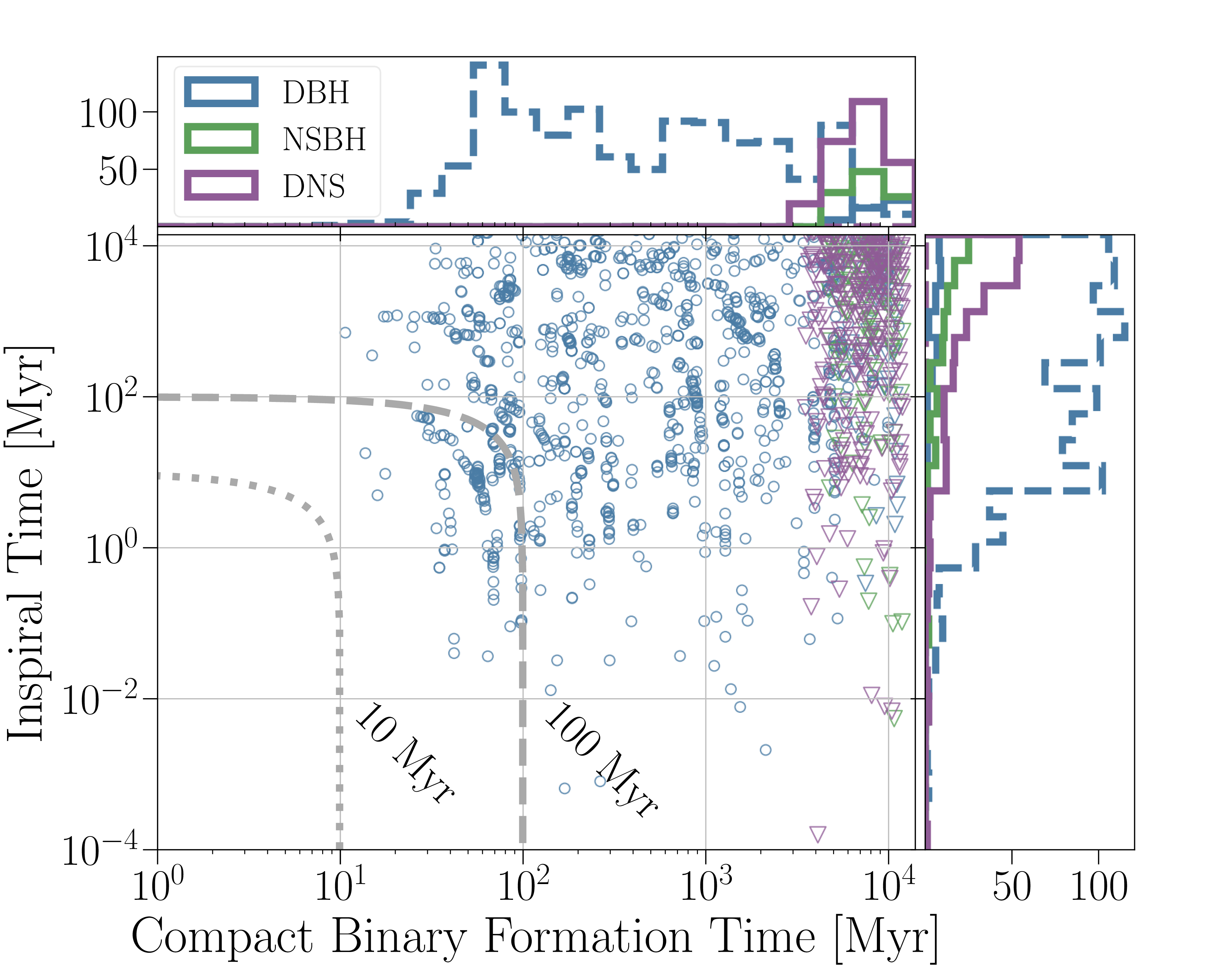
Time taken for double black hole (DHB, shown in blue), neutron star–black hole (NSBH, shown in green), and double neutron star (DNS, shown in purple) [bonus note] binaries to form and then inspiral to merge in globular cluster simulations. Circles and dashed histograms show results for the standard cluster model. Triangles and solids histograms show results when black holes are artificially removed. Figure 1 of a Zevin et al. (2019).
Isolated binaries
Considering isolated binaries, we need to work out how many binary neutron stars will merge close enough to a cluster to enrich it. This requires a couple of ingredients: (I) knowing how many binary neutron stars form, and (ii) working how many are still close to the cluster when they merge. Neutron stars will get kicks when they are born in supernova explosions, and these are enough to kick them out of the cluster. So long as they merge before they get too far, that’s OK for enrichment. Therefore we need to track both those that stay in the cluster, and those which leave but merge before getting too far. To estimate the number of enriching binary neutron stars, we simulated a populations of binary stars.
The evolution of binary neutron stars can be complicated. The neutron stars form from massive stars. In order for them to end up merging, they need to be in a close binary. This means that as the stars evolve and start to expand, they will transfer mass between themselves. This mass transfer can be stable, in which case the orbit widens, faster eventually shutting off the mass transfer, or it can be unstable, when the star expands leading to even more mass transfer (what’s really important is the rate of change of the size of the star compared to the Roche lobe). When mass transfer is extremely rapid, it leads to the formation of a common envelope: the outer layers of the donor ends up encompassing both the core of the star and the companion. Drag experienced in a common envelope can lead to the orbit shrinking, exactly as you’d want for a merger, but it can be too efficient, and the two stars may merge before forming two neutron stars. It’s also not clear what would happen in this case if there isn’t a clear boundary between the envelope and core of the donor star—it’s probable you’d just get a mess and the stars merging. We used COSMIC to see the effects of different assumptions about the physics:
- Model A: Our base model, which is in my opinion the least plausible. This assumes that helium stars can successfully survive a common envelope. Mass transfer from helium star will be especially important for our results, particularly what is called Case BB mass transfer [bonus note], which occurs once helium burning has finished in the core of a star, and is now burning is a shell outside the core.
- Model B: Here, we assume that stars without a clear core/envelope boundary will always merge during the common envelope. Stars burning helium in a shell lack a clear core/envelope boundary, and so any common envelopes formed from Case BB mass transfer will result in the stars merging (and no binary neutron star forming). This is a pessimistic model in terms of predicting rates.
- Model C: The same as Model A, but we use prescriptions from Tauris, Langer & Podsiadlowski (2015) for the orbital evolution and mass loss for mass transfer. These results show that mass transfer from helium stars typically proceeds stably. This means we don’t need to worry about common envelopes from Case BB mass transfer. This is more optimistic in terms of rates.
- Model D: The same as Model C, except all stars which undergo Case BB mass transfer are assumed to become ultra-stripped. Since they have less material in their envelopes, we give them smaller supernova natal kicks, the same as electron capture supernovae.
All our models can produce some merging neutron stars within 100 million years. However, for Model B, this number is small, so that only a few percent of globular clusters would be enriched. For the others, it would be a few tens of percent, but not all. Model A gives the most enrichment. Model C and D are similar, with Model D producing slightly less enrichment.

Post-supernova binary neutron star properties (systemic velocity 


Maybe?
Our results show that the r-process enrichment of globular clusters could be explained by binary neutron star mergers if binaries can survive Case BB mass transfer without merging. If Case BB mass transfer is typically unstable and somehow it is possible to survive a common envelope (Model A), ~30−90% of globular clusters should be enriched (depending upon their mass and size). This rate is consistent with consistent with current observations, but it is a stretch to imagine stars surviving common envelopes in this case. However, if Case BB mass transfer is stable (Models C and D), we still have ~10−70% of globular clusters should be enriched. This could plausibly explain everything! If we can measure the enrichment in more clusters and accurately pin down the fraction which are enriched, we may learn something important about how binaries interact.
However, for our idea to work, we do need globular clusters to form stars over an extended period of time. If there’s no gas around to absorb the material ejected from binary neutron star mergers and then form new stars, we have not cracked the problem. The plot below shows that the build up of enriching material happens at around 40 million years after the initial start formation. This is when we need the gas to be around. If this is not the case, we need a different method of enrichment.
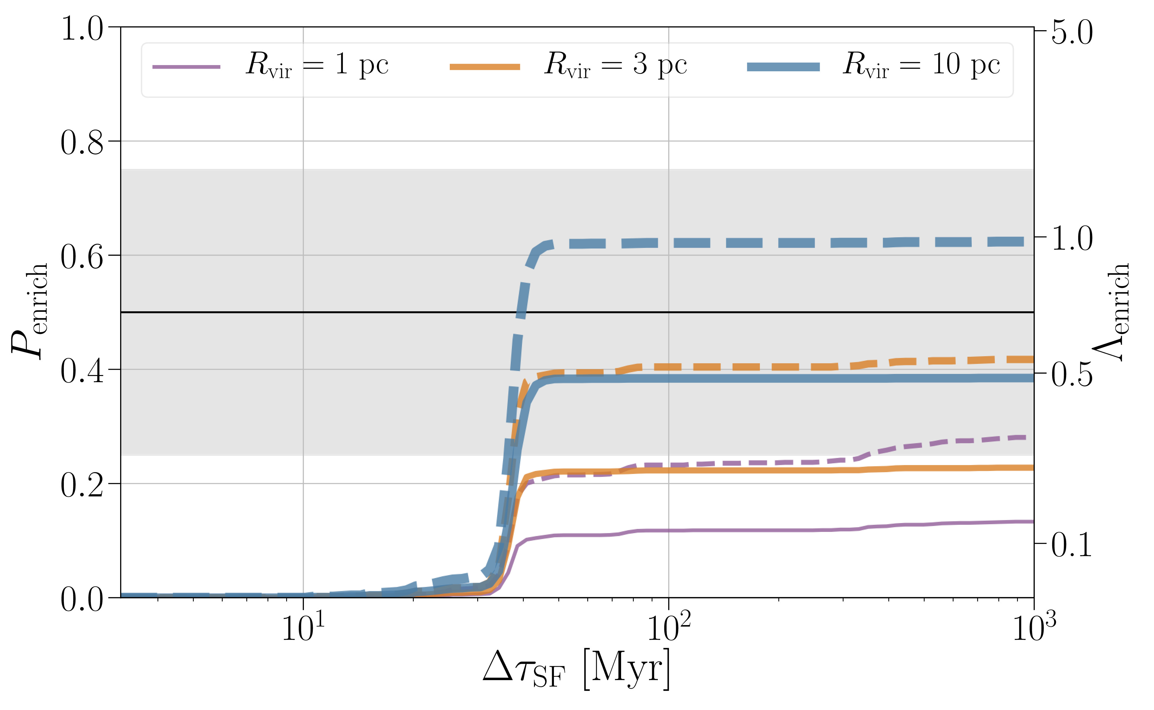
Probability of cluster enrichment 


It may be interesting to look again at r-process enrichment from supernova.
arXiv: arXiv:1906.11299 [astro-ph.HE]
Journal: Astrophysical Journal; 886(1):4(16); 2019 [bonus note]
Alternative tile: The Europium Report
Bonus notes
Hidden pulsars and GW190425
The most recent gravitational-wave detection, GW190425, comes from a binary neutron star system of an unusually high mass. It’s mass is much higher than the population of binary neutron stars observed in our Galaxy. One explanation for this could be that it represents a population which is short lived, and we’d be unlikely to spot one in our Galaxy, as they’re not around for long. Consequently, the same physics may be important both for this study of globular clusters and for explaining GW190425.
Gravitational-wave sources and dynamical formation
The question of how do binary neutron stars form is important for understanding gravitational-wave sources. The question of whether dynamically formed binary neutron stars could be a significant contribution to the overall rate was recently studied in detail in a paper led by Northwestern PhD student Claire Ye. The conclusions of this work was that the fraction of binary neutron stars formed dynamically in globular clusters was tiny (in agreement with our results). Only about 0.001% of binary neutron stars we observe with gravitational waves would be formed dynamically in globular clusters.
Double vs binary
In this paper we use double black hole = DBH and double neutron star = DNS instead of the usual binary black hole = BBH and binary neutron star = BNS from gravitational-wave astronomy. The terms mean the same. I will use binary instead of double here as B is worth more than D in Scrabble.
Mass transfer cases
The different types of mass transfer have names which I always forget. For regular stars we have:
- Case A is from a star on the main sequence, when it is burning hydrogen in its core.
- Case B is from a star which has finished burning hydrogen in its core, and is burning hydrogen in shell/burning helium in the core.
- Case C is from a start which has finished core helium burning, and is burning helium in a shell. The star will now have carbon it its core, which may later start burning too.
The situation where mass transfer is avoided because the stars are well mixed, and so don’t expand, has also been referred to as Case M. This is more commonly known as (quai)chemically homogenous evolution.
If a star undergoes Case B mass transfer, it can lose its outer hydrogen-rich layers, to leave behind a helium star. This helium star may subsequently expand and undergo a new phase of mass transfer. The mass transfer from this helium star gets named similarly:
- Case BA is from the helium star while it is on the helium main sequence burning helium in its core.
- Case BB is from the helium star once it has finished core helium burning, and may be burning helium in a shell.
- Case BC is from the helium star once it is burning carbon.
If the outer hydrogen-rich layers are lost during Case C mass transfer, we are left with a helium star with a carbon–oxygen core. In this case, subsequent mass transfer is named as:
- Case CB if helium shell burning is on-going. (I wonder if this could lead to fast radio bursts?)
- Case CC once core carbon burning has started.
I guess the naming almost makes sense. Case closed!
Page count
Don’t be put off by the length of the paper—the bibliography is extremely detailed. Michael was exceedingly proud of the number of references. I think it is the most in any non-review paper of mine!

 as calculated by
  ,
, is the likelihood for data
  (the number of observations and their chirp mass distribution in our case),
  are our parameters (natal kick, etc.), and the angular brackets indicate the average over the population parameters. In statistics terminology, this is the variance of the
 , the common envelope efficiency
  , the Wolf–Rayet mass loss rate
  , and the luminous blue variable mass loss rate
  . There is an anticorrealtion between
  and
and 
 as following a Maxwell–Boltzmann distribution,
 ,
, is not the same as this, however, as we assume some of the material ejected by the supernova falls back, reducing the over kick. The final natal kick is
 ,
, is the fraction that falls back, taken from
  and the probability of falling in each chirp mass bin
  (we factor measurement uncertainty into this). Our observations are the the total number of detections
  and the number in each chirp mass bin
  (
( ). The likelihood is the probability of these observations given the model predictions. We can split the likelihood into two pieces, one for the rate, and one for the chirp mass distribution,
 .
.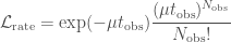 ,
, is the total observing time. For the chirp mass likelihood, we the probability of getting a number of detections in each bin, given the predicted fractions. This is given by a
 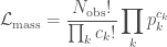 .
.![\displaystyle F_{ij} = \mu t_\mathrm{obs} \left[ \frac{1}{\mu^2} \frac{\partial \mu}{\partial \lambda_i} \frac{\partial \mu}{\partial \lambda_j} + \sum_k\frac{1}{p_k} \frac{\partial p_k}{\partial \lambda_i} \frac{\partial p_k}{\partial \lambda_j} \right]](https://s0.wp.com/latex.php?latex=%5Cdisplaystyle+F_%7Bij%7D+%3D+%5Cmu+t_%5Cmathrm%7Bobs%7D+%5Cleft%5B+%5Cfrac%7B1%7D%7B%5Cmu%5E2%7D+%5Cfrac%7B%5Cpartial+%5Cmu%7D%7B%5Cpartial+%5Clambda_i%7D%C2%A0%5Cfrac%7B%5Cpartial+%5Cmu%7D%7B%5Cpartial+%5Clambda_j%7D%C2%A0+%2B+%5Csum_k%5Cfrac%7B1%7D%7Bp_k%7D+%5Cfrac%7B%5Cpartial+p_k%7D%7B%5Cpartial+%5Clambda_i%7D%C2%A0%5Cfrac%7B%5Cpartial+p_k%7D%7B%5Cpartial+%5Clambda_j%7D+%5Cright%5D&bg=ffffff&fg=444444&s=0&c=20201002) .
. . Therefore, we can see that the measurement uncertainty defined by the inverse of the Fisher information matrix, scales on average as
  .
. and
and  are the same as their expectation values. The second-order derivatives are given by the expression we have worked out for the Fisher information matrix. Therefore, in the region around the maximum likelihood point, the Fisher information matrix encodes all the relevant information about the shape of the likelihood.
 , you’ll see that the distribution basically becomes a delta function at the maximum likelihood values. To check that our
  was large enough, we verified that higher-order derivatives were still small.