The space-based observatory LISA will detect gravitational waves from massive black holes (giant black holes residing in the centres of galaxies). One particularly interesting signal will come from the inspiral of a regular stellar-mass black hole into a massive black hole. These are called extreme mass-ratio inspirals (or EMRIs, pronounced emries, to their friends) [bonus note]. We have never observed such a system. This means that there’s a lot we have to learn about them. In this work, we systematically investigated the prospects for observing EMRIs. We found that even though there’s a wide range in predictions for what EMRIs we will detect, they should be a safe bet for the LISA mission.

Artistic impression of the spacetime for an extreme-mass-ratio inspiral, with a smaller stellar-mass black hole orbiting a massive black hole. This image is mandatory when talking about extreme-mass-ratio inspirals. Credit: NASA
LISA & EMRIs
My previous post discussed some of the interesting features of EMRIs. Because of the extreme difference in masses of the two black holes, it takes a long time for them to complete their inspiral. We can measure tens of thousands of orbits, which allows us to make wonderfully precise measurements of the source properties (if we can accurately pick out the signal from the data). Here, we’ll examine exactly what we could learn with LISA from EMRIs [bonus note].
First we build a model to investigate how many EMRIs there could be. There is a lot of astrophysics which we are currently uncertain about, which leads to a large spread in estimates for the number of EMRIs. Second, we look at how precisely we could measure properties from the EMRI signals. The astrophysical uncertainties are less important here—we could get a revolutionary insight into the lives of massive black holes.
The number of EMRIs
To build a model of how many EMRIs there are, we need a few different inputs:
- The population of massive black holes
- The distribution of stellar clusters around massive black holes
- The range of orbits of EMRIs
We examine each of these in turn, building a more detailed model than has previously been constructed for EMRIs.
We currently know little about the population of massive black holes. This means we’ll discover lots when we start measuring signals (yay), but it’s rather inconvenient now, when we’re trying to predict how many EMRIs there are (boo). We take two different models for the mass distribution of massive black holes. One is based upon a semi-analytic model of massive black hole formation, the other is at the pessimistic end allowed by current observations. The semi-analytic model predicts massive black hole spins around 0.98, but we also consider spins being uniformly distributed between 0 and 1, and spins of 0. This gives us a picture of the bigger black hole, now we need the smaller.
Observations show that the masses of massive black holes are correlated with their surrounding cluster of stars—bigger black holes have bigger clusters. We consider four different versions of this trend: Gültekin et al. (2009); Kormendy & Ho (2013); Graham & Scott (2013), and Shankar et al. (2016). The stars and black holes about a massive black hole should form a cusp, with the density of objects increasing towards the massive black hole. This is great for EMRI formation. However, the cusp is disrupted if two galaxies (and their massive black holes) merge. This tends to happen—it’s how we get bigger galaxies (and black holes). It then takes some time for the cusp to reform, during which time, we don’t expect as many EMRIs. Therefore, we factor in the amount of time for which there is a cusp for massive black holes of different masses and spins.

That’s a nice galaxy you have there. It would be a shame if it were to collide with something… Hubble image of The Mice. Credit: ACS Science & Engineering Team.
Given a cusp about a massive black hole, we then need to know how often an EMRI forms. Simulations give us a starting point. However, these only consider a snap-shot, and we need to consider how things evolve with time. As stellar-mass black holes inspiral, the massive black hole will grow in mass and the surrounding cluster will become depleted. Both these effects are amplified because for each inspiral, there’ll be many more stars or stellar-mass black holes which will just plunge directly into the massive black hole. We therefore need to limit the number of EMRIs so that we don’t have an unrealistically high rate. We do this by adding in a couple of feedback factors, one to cap the rate so that we don’t deplete the cusp quicker than new objects will be added to it, and one to limit the maximum amount of mass the massive black hole can grow from inspirals and plunges. This gives us an idea for the total number of inspirals.
Finally, we calculate the orbits that EMRIs will be on. We again base this upon simulations, and factor in how the spin of the massive black hole effects the distribution of orbital inclinations.
Putting all the pieces together, we can calculate the population of EMRIs. We now need to work out how many LISA would be able to detect. This means we need models for the gravitational-wave signal. Since we are simulating a large number, we use a computationally inexpensive analytic model. We know that this isn’t too accurate, but we consider two different options for setting the end of the inspiral (where the smaller black hole finally plunges) which should bound the true range of results.

Number of EMRIs for different size massive black holes in different astrophysical models. M1 is our best estimate, the others explore variations on this. M11 and M12 are designed to be cover the extremes, being the most pessimistic and optimistic combinations. The solid and dashed lines are for two different signal models (AKK and AKS), which are designed to give an indication of potential variation. They agree where the massive black hole is not spinning (M10 and M11). The range of masses is similar for all models, as it is set by the sensitivity of LISA. We can detect higher mass systems assuming the AKK signal model as it includes extra inspiral close to highly spinning black holes: for the heaviest black holes, this is the only part of the signal at high enough frequency to be detectable. Figure 8 of Babak et al. (2017).
Allowing for all the different uncertainties, we find that there should be somewhere between 1 and 4200 EMRIs detected per year. (The model we used when studying transient resonances predicted about 250 per year, albeit with a slightly different detector configuration, which is fairly typical of all the models we consider here). This range is encouraging. The lower end means that EMRIs are a pretty safe bet, we’d be unlucky not to get at least one over the course of a multi-year mission (LISA should have at least four years observing). The upper end means there could be lots—we might actually need to worry about them forming a background source of noise if we can’t individually distinguish them!
EMRI measurements
Having shown that EMRIs are a good LISA source, we now need to consider what we could learn by measuring them?
We estimate the precision we will be able to measure parameters using the Fisher information matrix. The Fisher matrix measures how sensitive our observations are to changes in the parameters (the more sensitive we are, the better we should be able to measure that parameter). It should be a lower bound on actual measurement precision, and well approximate the uncertainty in the high signal-to-noise (loud signal) limit. The combination of our use of the Fisher matrix and our approximate signal models means our results will not be perfect estimates of real performance, but they should give an indication of the typical size of measurement uncertainties.
Given that we measure a huge number of cycles from the EMRI signal, we can make really precise measurements of the the mass and spin of the massive black hole, as these parameters control the orbital frequencies. Below are plots for the typical measurement precision from our Fisher matrix analysis. The orbital eccentricity is measured to similar accuracy, as it influences the range of orbital frequencies too. We also get pretty good measurements of the the mass of the smaller black hole, as this sets how quickly the inspiral proceeds (how quickly the orbital frequencies change). EMRIs will allow us to do precision astronomy!

Distribution of (one standard deviation) fractional uncertainties for measurements of the massive black hole (redshifted) mass 

Distribution of (one standard deviation) uncertainties for measurements of the massive black hole spin 
Now, before you get too excited that we’re going to learn everything about massive black holes, there is one confession I should make. In the plot above I show the measurement accuracy for the redshifted mass of the massive black hole. The cosmological expansion of the Universe causes gravitational waves to become stretched to lower frequencies in the same way light is (this makes visible light more red, hence the name). The measured frequency is 


Distribution of (one standard deviation) fractional uncertainties for measurements of the luminosity distance 
The plot above shows the fractional uncertainty on the distance. We don’t measure this too well, as it is determined from the amplitude of the signal, rather than its frequency components. The situation is much as for LIGO. The larger uncertainties on the distance will dominate the overall uncertainty on the black hole masses. We won’t be getting all these to fractions of a percent. However, that doesn’t mean we can’t still figure out what the distribution of masses looks like!
One of the really exciting things we can do with EMRIs is check that the signal matches our expectations for a black hole in general relativity. Since we get such an excellent map of the spacetime of the massive black hole, it is easy to check for deviations. In general relativity, everything about the black hole is fixed by its mass and spin (often referred to as the no-hair theorem). Using the measured EMRI signal, we can check if this is the case. One convenient way of doing this is to describe the spacetime of the massive object in terms of a multipole expansion. The first (most important) terms gives the mass, and the next term the spin. The third term (the quadrupole) is set by the first two, so if we can measure it, we can check if it is consistent with the expected relation. We estimated how precisely we could measure a deviation in the quadrupole. Fortunately, for this consistency test, all factors from redshifting cancel out, so we can get really detailed results, as shown below. Using EMRIs, we’ll be able to check for really small differences from general relativity!

Distribution of (one standard deviation) of uncertainties for deviations in the quadrupole moment of the massive object spacetime 
In summary: EMRIS are awesome. We’re not sure how many we’ll detect with LISA, but we’re confident there will be some, perhaps a couple of hundred per year. From the signals we’ll get new insights into the masses and spins of black holes. This should tell us something about how they, and their surrounding galaxies, evolved. We’ll also be able to do some stringent tests of whether the massive objects are black holes as described by general relativity. It’s all pretty exciting, for when LISA launches, which is currently planned about 2034…

One of the most valuable traits a student or soldier can have: patience. Credit: Sony/Marvel
arXiv: 1703.09722 [gr-qc]
Journal: Physical Review D; 477(4):4685–4695; 2018
Conference proceedings: 1704.00009 [astro-ph.GA] (from when work was still in-progress)
Estimated number of Marvel films before LISA launch: 48 (starting with Ant-Man and the Wasp)
Bonus notes
Hyphenation
Is it “extreme-mass-ratio inspiral”, “extreme mass-ratio inspiral” or “extreme mass ratio inspiral”? All are used in the literature. This is one of the advantage of using “EMRI”. The important thing is that we’re talking about inspirals that have a mass ratio which is extreme. For this paper, we used “extreme mass-ratio inspiral”, but when I first started my PhD, I was first introduced to “extreme-mass-ratio inspirals”, so they are always stuck that way in my mind.
I think hyphenation is a bit of an art, and there’s no definitive answer here, just like there isn’t for superhero names, where you can have Iron Man, Spider-Man or Iceman.
Science with LISA
This paper is part of a series looking at what LISA could tells us about different gravitational wave sources. So far, this series covers
- Massive black hole binaries
- Cosmological phase transitions
- Standard sirens (for measuring the expansion of the Universe)
- Inflation
- Extreme-mass-ratio inspirals
You’ll notice there’s a change in the name of the mission from eLISA to LISA part-way through, as things have evolved. (Or devolved?) I think the main take-away so far is that the cosmology group is the most enthusiastic.
 , one for polar (north/south if we think of the spin of the massive black hole like the rotation of the Earth) motion
  and one for axial (around in the east/west direction) motion. As gravitational waves are emitted, and the orbit shrinks, these frequencies evolve. The animation above, made by
 –
– plane. Credit: Rob Cole
 which is defined below. Figure 4 of
  .
. . What should this depend on? There are three ingredients. First, the rate of change of this constant
  on the resonant orbit. Second, the time spent on resonance
  .
. . By varying
 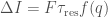 ,
, . Now, we know the pieces, we can try to figure out what the pieces are.
 : the smaller the stellar-mass black hole is relative to the massive one, the smaller
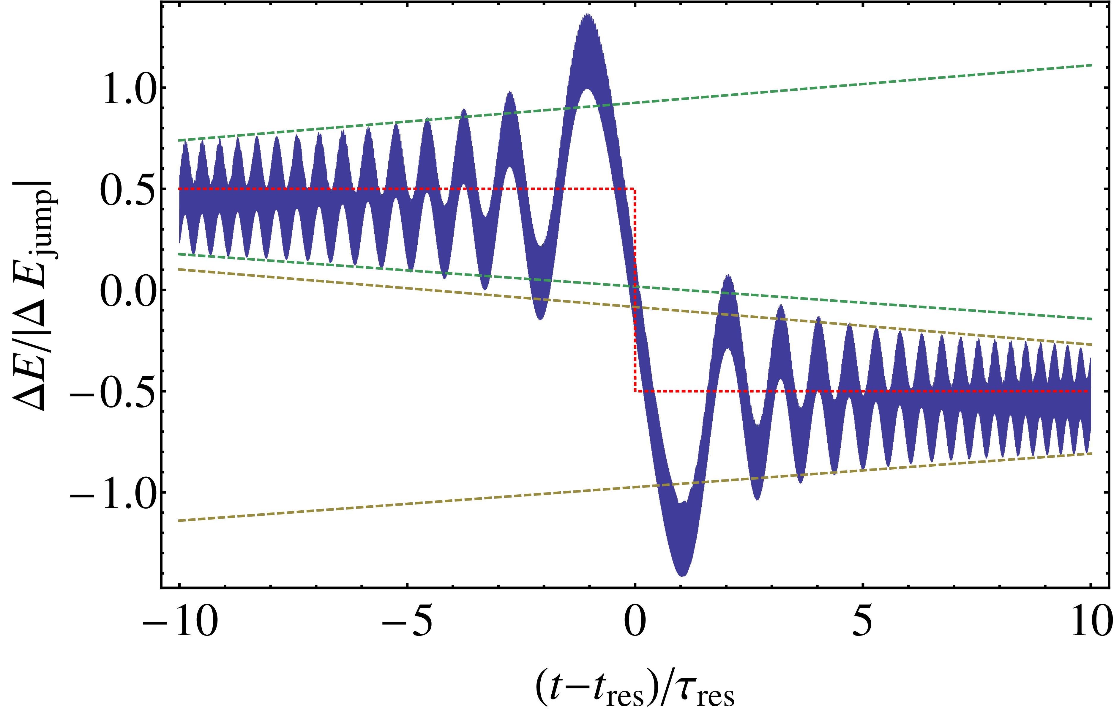
  , which is zero exactly on resonance. If this is evolving at rate
  , then the resonance timescale is
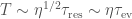
![\displaystyle \tau_\mathrm{res} = \left[\frac{2\pi}{\dot{\Omega}}\right]^{1/2}](https://s0.wp.com/latex.php?latex=%5Cdisplaystyle+%5Ctau_%5Cmathrm%7Bres%7D+%3D+%5Cleft%5B%5Cfrac%7B2%5Cpi%7D%7B%5Cdot%7B%5COmega%7D%7D%5Cright%5D%5E%7B1%2F2%7D&bg=ffffff&fg=444444&s=0&c=20201002) .
. and the long evolution timescale
  :
: .
. , we need to do some quite involved maths (given in Appendix B of the
  and
and  ) have smaller jumps than lower-order ones. This makes sense, as higher-order resonances come closer to covering all the points in the space, and so are more like averaging over the entire space. Second, jumps are larger for higher eccentricity orbits. This also makes sense, as you can’t have resonances for circular (zero eccentricity orbits) as there’s no radial frequency, so the size of the jumps must tend to zero. We’ll see that these two points are important when it comes to observational consequences of transient resonances.
 are not important because the spacetime is axisymmetric. The equations are exactly identical for all values of the the axial angle
  , so it doesn’t matter where you are (or if you keep cycling over the same spot) for the evolution of the EMRI.