Rob Cole

Extreme-mass-ratio inspirals (EMRIs for short) are a promising source for the planned space-borne gravitational-wave observatory LISA. To detect and analyse them we need accurate models for the signals, which are exquisitely intricate. In this paper, we investigated a feature, transient resonances, which have not previously included in our models. They are difficult to incorporate, but can have a big impact on the signal. Fortunately, we find that we can still detect the majority of EMRIs, even without including resonances. Phew!

EMRIs and orbits

EMRIs are a beautiful gravitational wave source. They occur when a stellar-mass black hole slowly inspirals into a massive black hole (as found in the centre of galaxies). The massive black hole can be tens of thousands or millions of times more massive than the stellar-mass black hole (hence extreme mass ratio). This means that the inspiral is slow—we can potentially measure tens of thousands of orbits. This is both the blessing and the curse of EMRIs. The huge numbers of cycles means that we can closely follow the inspiral, and build a detailed map of the massive black hole’s spacetime. EMRIs will give us precision measurements of the properties of massive black holes. However, to do this, we need to be able to find the EMRI signals in the data, we need models which can match the signals over all these cycles. Analysing EMRIs is a huge challenge.

EMRI orbits are complicated. At any moment, the orbit can be described by three orbital frequencies: one for radial (in/out) motion $\Omega_r$ , one for polar (north/south if we think of the spin of the massive black hole like the rotation of the Earth) motion $\Omega_\theta$ and one for axial (around in the east/west direction) motion. As gravitational waves are emitted, and the orbit shrinks, these frequencies evolve. The animation above, made by Steve Drasco, illustrates the evolution of an EMRI. Every so often, so can see the pattern freeze—the orbits stays in a constant shape (although this still rotates). This is a transient resonance. Two of the orbital frequencies become commensurate (so we might have 3 north/south cycles and 2 in/out cycles over the same period [bonus note])—this is the resonance. However, because the frequencies are still evolving, we don’t stay locked like this is forever—which is why the resonance is transient. To calculate an EMRI, you need to know how the orbital frequencies evolve.

The evolution of an EMRI is slow—the time taken to inspiral is much longer than the time taken to complete one orbit. Therefore, we can usually split the problem of calculating the trajectory of an EMRI into two parts. On short timescales, we can consider orbits as having fixed frequencies. On long timescale, we can calculate the evolution by averaging over many orbits. You might see the problem with this—around resonances, this averaging breaks down. Whereas normally averaging over many orbits means averaging over a complicated trajectory that hits pretty much all possible points in the orbital range, on resonance, you just average over the same bit again and again. On resonance, terms which usually average to zero can become important. Éanna Flanagan and Tanja Hinderer first pointed out that around resonances the usual scheme (referred to as the adiabatic approximation) doesn’t work.

A non-resonant EMRI orbit in three dimensions (left) and two dimensions (right), ignoring the rotation in the axial direction. A non-resonant orbit will eventually fill the $r$ – $\theta$ plane. Credit: Rob Cole

For comparison, a resonant EMRI orbit. A 2:3 resonance traces the same parts of the $r$ – $\theta$ plane over and over. Credit: Rob Cole

Around a resonance, the evolution will be enhanced or decreased a little relative to the standard adiabatic evolution. We get a kick. This is only small, but because we observe EMRIs for so many orbits, a small difference can grow to become a significant difference later on. Does this mean that we won’t be able to detect EMRIs with our standard models? This was a concern, so back at the end of PhD I began to investigate [bonus note]. The first step is to understand the size of the kick.

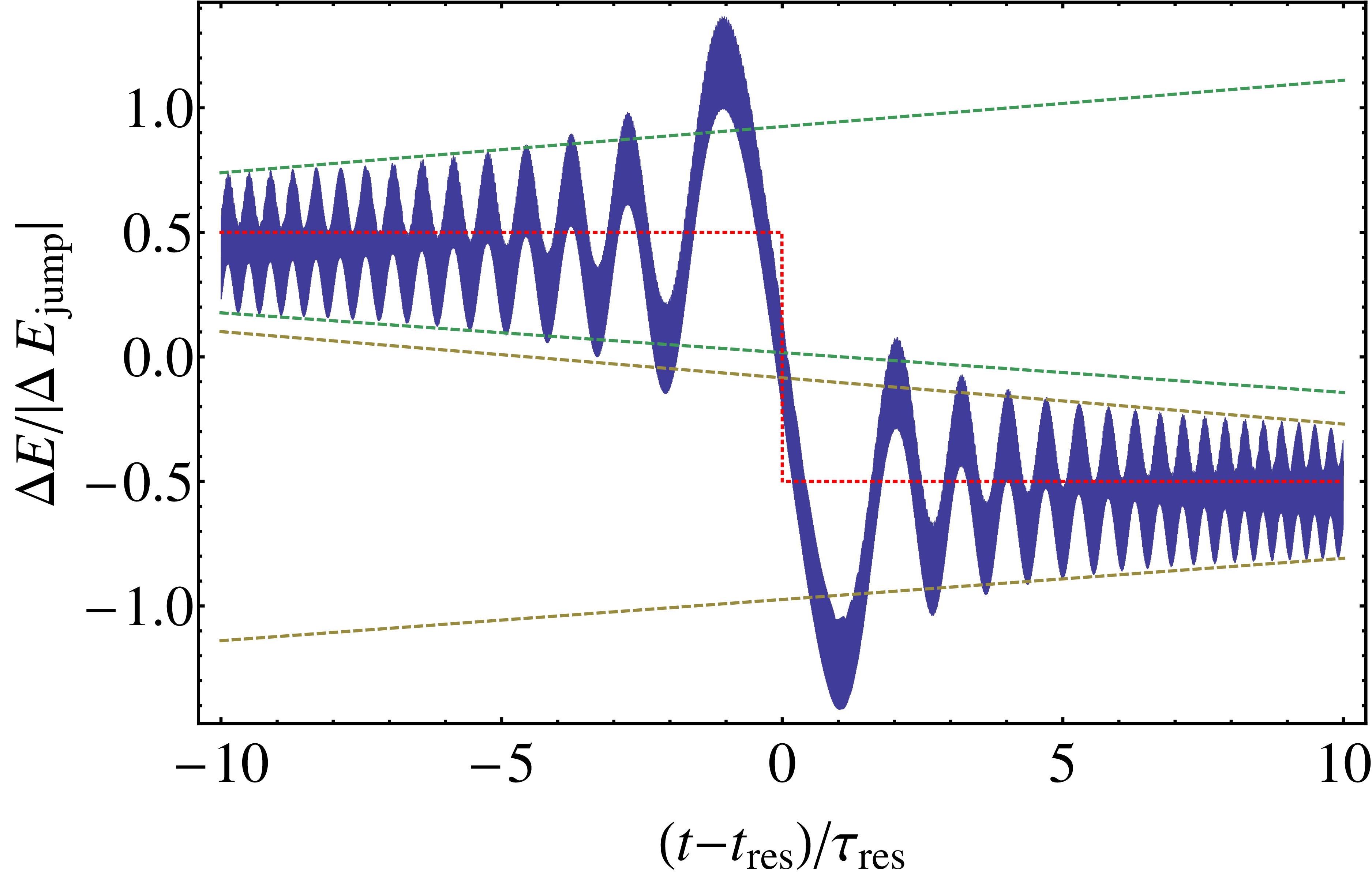
A jump in the orbital energy across a 2:3 resonance. The plot shows the difference between the approximate adiabatic evolution and the instantaneous evolution including the resonance. The thickness of the blue line is from oscillations on the orbital timescale which is too short to resolve here. The dotted red line shows the fitted size of the jump. Time is measured in terms of the resonance time $\tau_\mathrm{res}$ which is defined below. Figure 4 of Berry et al. (2016).

Resonance kicks

If there were no gravitational waves, the orbit would not evolve, it would be fixed. The orbit could then be described by a set of constants of motion. The most commonly used when describing orbits about black holes are the energy, angular momentum and Carter constant. For the purposes of this blog, we’ll not worry too much about what these constants are, we’ll just consider some constant $I$ .

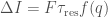
The resonance kick is a change in this constant $\Delta I$ . What should this depend on? There are three ingredients. First, the rate of change of this constant $F$ on the resonant orbit. Second, the time spent on resonance $\tau_\mathrm{res}$ . The bigger these are, the bigger the size of the jump. Therefore,

$|\Delta I| \propto F \tau_\mathrm{res}$ .

However, the jump could be positive or negative. This depends upon the relative phase of the radial and polar motion [bonus note]—for example, do they both reach their maximum point at the same time, or does one lag behind the other? We’ll call this relative phase $q$ . By varying $q$ we explore we can get our resonant trajectory to go through any possible point in space. Therefore, averaging over $q$ should get us back to the adiabatic approximation: the average value of $\Delta I$ must be zero. To complete our picture for the jump, we need a periodic function of the phase,

$\Delta I = F \tau_\mathrm{res} f(q)$ ,

with $\langle f(q) \rangle_q = 0$ . Now, we know the pieces, we can try to figure out what the pieces are.

The rate of change $F$ is proportional the mass ratio $\eta \ll 1$ : the smaller the stellar-mass black hole is relative to the massive one, the smaller $F$ is. The exact details depend upon gravitational self-force calculations, which we’ll skip over, as they’re pretty hard, but they are the same for all orbits (resonant or not).

We can think of the resonance timescale either as the time for the orbital frequencies to drift apart or the time for the orbit to start filling the space again (so that it’s safe to average). The two pictures yield the same answer—there’s a fuller explanation in Section III A of the paper. To define the resonance timescale, it is useful to define the frequency $\Omega = n_r \Omega_r - n_\theta \Omega_\theta$ , which is zero exactly on resonance. If this is evolving at rate $\dot{\Omega}$ , then the resonance timescale is

$\displaystyle \tau_\mathrm{res} = \left[\frac{2\pi}{\dot{\Omega}}\right]^{1/2}$ .

This bridges the two timescales that usually define EMRIs: the short orbital timescale $T$ and the long evolution timescale $\tau_\mathrm{ev}$ :

$T \sim \eta^{1/2} \tau_\mathrm{res} \sim \eta \tau_\mathrm{ev}$ .

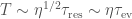
To find the form of for $f(q)$ , we need to do some quite involved maths (given in Appendix B of the paper) [bonus note]. This works by treating the evolution far from resonance as depending upon two independent times (effectively defining $T$ and $\tau_\mathrm{ev}$ ), and then matching the evolution close to resonance using an expansion in terms of a different time (something like $\tau_\mathrm{res}$ ). The solution shows that the jump depends sensitively upon the phase $q$ at resonance, which makes them extremely difficult to calculate.

We numerically evaluated the size of kicks for different orbits and resonances. We found a number of trends. First, higher-order resonances (those with larger $n_r$ and $n_\theta$ ) have smaller jumps than lower-order ones. This makes sense, as higher-order resonances come closer to covering all the points in the space, and so are more like averaging over the entire space. Second, jumps are larger for higher eccentricity orbits. This also makes sense, as you can’t have resonances for circular (zero eccentricity orbits) as there’s no radial frequency, so the size of the jumps must tend to zero. We’ll see that these two points are important when it comes to observational consequences of transient resonances.

Astrophysical EMRIs

Now we’ve figured out the impact of passing through a transient resonance, let’s look at what this means for detecting EMRIs. The jump can mean that the evolution post-resonance can soon become out of phase with that pre-resonance. We can’t match both parts with the same adiabatic template. This could significantly hamper our prospects for detection, as we’re limited to the bits of signal we can pick up between resonances.

We created an astrophysical population of simulated EMRIs. We used numerical simulations to estimate a plausible population of massive black holes and distribution of stellar-mass black holes insprialling into them. We then used adiabatic models to see how many LISA (or eLISA as it was called at the time) could potentially detect. We found there were ~510 EMRIs detectable (with a signal-to-noise ratio of 15 or above) for a two-year mission.

We then calculated how much the signal-to-noise ratio would be reduced by passing through transient resonances. The plot below shows the distribution of signal-to-noise ratio for the original population, ignoring resonances, and then after factoring in the reduction. There are now ~490 detectable EMRIs, a loss of 4%. We can still detect the majority of EMRIs!

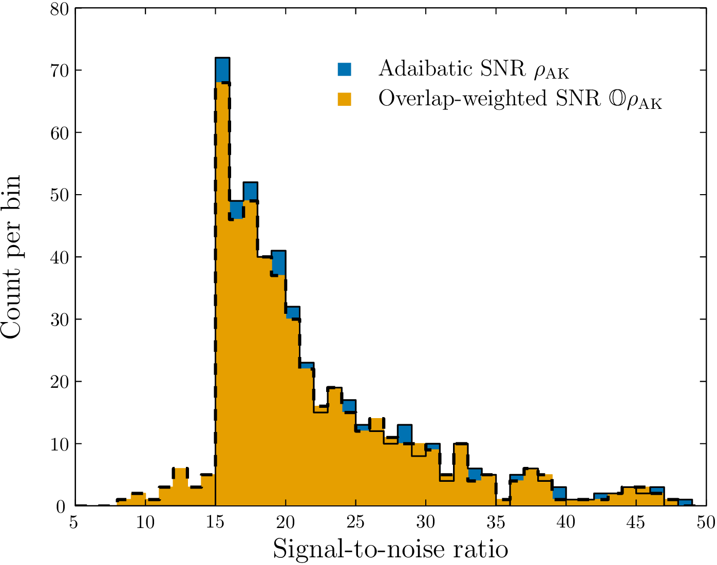
Distribution of signal-to-noise ratios for EMRIs. In blue (solid outline), we have the results ignoring transient resonances. In orange (dashed outline), we have the distribution including the reduction due to resonance jumps. Events falling below 15 are deemed to be undetectable. Figure 10 of Berry et al. (2016).

We were worried about the impact of transient resonances, we know that jumps can cause them to become undetectable, so why aren’t we seeing a bit effect in our population? The answer lies is in the trends we saw earlier. Jumps are large for low order resonances with high eccentricities. These were the ones first highlighted, as they are obviously the most important. However, low-order resonances are only encountered really close to the massive black hole. This means late in the inspiral, after we have already accumulated lots of signal-to-noise ratio. Losing a little bit of signal right at the end doesn’t hurt detectability too much. On top of this, gravitational wave emission efficiently damps down eccentricity. Orbits typically have low eccentricities by the time they hit low-order resonances, meaning that the jumps are actually quite small. Although small jumps lead to some mismatch, we can still use our signal templates without jumps. Therefore, resonances don’t hamper us (too much) in finding EMRIs!

This may seem like a happy ending, but it is not the end of the story. While we can detect EMRIs, we still need to be able to accurately infer their source properties. Features not included in our signal templates (like jumps), could bias our results. For example, it might be that we can better match a jump by using a template for a different black hole mass or spin. However, if we include jumps, these extra features could give us extra precision in our measurements. The question of what jumps could mean for parameter estimation remains to be answered.

arXiv: 1608.08951 [gr-qc]
Journal: Physical Review D; 94(12):124042(24); 2016
Conference proceedings: 1702.05481 [gr-qc] (only 2 pages—ideal for emergency journal club presentations)
Favourite jumpers: Woolly, Mario, Kangaroos

Bonus notes

Radial and polar only

When discussing resonances, and their impact on orbital evolution, we’ll only care about $\Omega_r$ – $\Omega_\theta$ resonances. Resonances with $\Omega_\phi$ are not important because the spacetime is axisymmetric. The equations are exactly identical for all values of the the axial angle $\phi$ , so it doesn’t matter where you are (or if you keep cycling over the same spot) for the evolution of the EMRI.

This, however, doesn’t mean that $\Omega_\phi$ resonances aren’t interesting. They can lead to small kicks to the binary, because you are preferentially emitting gravitational waves in one direction. For EMRIs this are negligibly small, but for more equal mass systems, they could have some interesting consequences as pointed out by Maarten van de Meent.

Extra time

I’m grateful to the Cambridge Philosophical Society for giving me some extra funding to work on resonances. If you’re a Cambridge PhD student, make sure to become a member so you can take advantage of the opportunities they offer.

Calculating jumps

The theory of how to evolve through a transient resonance was developed by Kevorkian and coauthors. I spent a long time studying these calculations before working up the courage to attempt them myself. There are a few technical details which need to be adapted for the case of EMRIs. I finally figured everything out while in Warsaw Airport, coming back from a conference. It was the most I had ever felt like a real physicist.

Transient resonances remind me of Spirographs. Thanks Frinkiac

Differing weights and differing measures—
the LORD detests them both. — Proverbs 20:10

As a New Year’s resolution, I thought I would try to write a post on each paper I have published. (I might try to go back and talk about my old papers too, but that might be a little too optimistic.) Handily, I have a paper that was published in Classical & Quantum Gravity on Thursday, so let’s get on with it, and hopefully 2015 will deliver those hoverboards soon.

This paper was written in collaboration with my old officemates, Chris Moore and Rob Cole, and originates from my time in Cambridge. We were having a weekly group meeting (surreptitiously eating cake—you’re not meant to eat in the new meeting rooms) and discussing what to do for the upcoming open afternoon. Posters are good as you can use them to decorate your office afterwards, so we decided on making one on gravitational-wave astronomy. Gravitational waves come in a range of frequencies, just like light (electromagnetic radiation). You can observe different systems with different frequencies, but you need different instruments to do so. For light, the range is from high frequency gamma rays (observed with satellites like Fermi) to low frequency radio waves (observed with telescopes like those at Jodrell Bank or Arecibo), with visible light (observed with Hubble or your own eyes) in the middle. Gravitational waves also have a spectrum, ground-based detectors like LIGO measure the higher frequencies, pulsar timing arrays measure the lower frequencies, and space-borne detectors like eLISA measure stuff in the middle. We wanted a picture that showed the range of each instrument and the sources they could detect, but we couldn’t find a good up-to-date one. Chris is not one to be put off by a challenge (especially if it’s a source of procrastination), so he decided to have a go at making one himself. How hard could it be? We never made that poster, but we did end up with a paper.

When talking about gravitational-wave detectors, you normally use a sensitivity curve. This shows how sensitive it is at a given frequency: you plot a graph with the sensitivity curve on, and then plot the spectrum of the source you’re interested in on the same graph. If your source is above the sensitivity curve, you can detect it (yay), but if it lies below it, then you can’t pick it out from the noise (boo). Making a plot with lots of sensitivity curves on sounds simple: you look up the details for lots of detectors, draw them together and add a few sources. However, there are lots of different conventions for how you actually measure sensitivity, and they’re frequently muddled up! We were rather confused by the whole thing, but eventually (after the open afternoon had flown by), we figured things out and made our picture. So we wouldn’t forget, we wrote up the different conventions, why you might want to use each, and how to convert between them; these notes became the paper. We also thought it would be handy to have a website where you could make your own plot, picking which detectors and sources you wanted to include. Rob also likes a challenge (especially if it’s a source of procrastination), so he set about making such a thing. I think it turned out rather well!

That’s the story of the paper. It explains different conventions for characterising gravitational-wave detectors and sources, and gives some examples. If you’d actually like to know some of the details, I’ll give a little explanation now, if not, just have a look at the pretty plots below (or, if looking for your own source of procrastination, have a go at Space Time Quest, a game where you try to build the most sensitive detector).

There are three common conventions in use for sensitivity-curve plots: the characteristic strain, the amplitude spectral density and the energy density.

You might wonder why we don’t just directly use the amplitude of the wave? Gravitational waves are a stretching and squashing of spacetime, so you can characterise how much they stretch and squeeze things and use that to describe the size of your waves. The sensitivity of your detector is then how much various sources of noise cause a similar wibbling. The amplitude of the wave is really, really small, so it’s difficult to detect, but if you were to consider observations over a time interval instead of just one moment, it’s easier to spot a signal: hints that there might be a signal add up until you’re certain that it’s there. The characteristic strain is a way of modifying the amplitude to take into account how we add up the signal. It’s especially handy, as if you make a log–log plot (such that the space between 1 and 10 is the same as between 10 and 100, etc.), then the area between the characteristic strain of your source and the detector sensitivity curve gives you a measure of the signal-to-noise ratio, a measure of how loud (how detectable) a signal is.

Gravitational-wave sensitivity-curve plot using characteristic strain. The area between the detector’s curve and the top of the box for a source indicates how loud that signal would be.

The characteristic strain is handy for quickly working out how loud a signal is, but it’s not directly related to anything we measure. The noise in a detector is usually described by its power spectral density or PSD. This tells you how much wibbling there is on average. Actually, it tells you the average amount of wibbling squared. The square root of the PSD is the amplitude spectral density or ASD. This gives a handy indication of the sensitivity of your detector, which is actually related to what you measure.

Gravitational-wave sensitivity-curve plot using the square root of the power spectral density (the amplitude spectral density).

The PSD is tied to the detector, but isn’t too relevant to the actual waves. An interesting property of the waves is how much energy they carry. We talk about this in terms of the energy density, the energy per unit volume. Cosmologists love this, and to make things easy for themselves, they like to divide energy densities by the amount that would make the Universe flat. (If you’ve ever wondered what astrophysicists mean when they say the Universe is about 70% dark energy and about 25% dark matter, they’re using these quantities). To make things even simpler, they like to multiply this quantity by something related to the Hubble constant (which measures the expansion rate of the Universe), as this means things don’t change if you tweak the numbers describing how the Universe evolves. What you’re left with is a quantity $\Omega h_{100}^2$ that is really convenient if you’re a cosmologist, but a pain for anyone else. It does have the advantage of making the pulsar timing arrays look more sensitive though.

Gravitational-wave sensitivity-curve plot using the energy density that cosmologists love. The proper name of the plotted quantity is the critical energy density per logarithmic frequency interval multiplied by the reduced Hubble constant squared. I prefer Bob.

We hope that the paper will be useful for people (like us), who can never remember what the conventions are (and why). There’s nothing new (in terms of results) in this paper, but I think it’s the first time all this material has been collected together in one place. If you ever need to make a poster about gravitational waves, I know where you can find a good picture.

arXiv: 1408.0740 [gr-qc]
Journal: Classical & Qunatum Gravity; 32(1):015014(25); 2015
Website: Gravitational Wave Sensitivity Curve Plotter
Procrastination score: TBC