An introduction to probability: Inference and learning from data

October 18, 2014February 7, 2015 / CPLB / Leave a comment

Probabilities are a way of quantifying your degree of belief. The more confident you are that something is true, the larger the probability assigned to it, with 1 used for absolute certainty and 0 used for complete impossibility. When you get new information that updates your knowledge, you should revise your probabilities. This is what we do all the time in science: we perform an experiment and use our results to update what we believe is true. In this post, I’ll explain how to update your probabilities, just as Sherlock Holmes updates his suspicions after uncovering new evidence.

Taking an umbrella

Imagine that you are a hard-working PhD student and you have been working late in your windowless office. Having finally finished analysing your data, you decide it’s about time to go home. You’ve been trapped inside so long that you no idea what the weather is like outside: should you take your umbrella with you? What is the probability that it is raining? This will depend upon where you are, what time of year it is, and so on. I did my PhD in Cambridge, which is one of the driest places in England, so I’d be confident that I wouldn’t need one. We’ll assume that you’re somewhere it doesn’t rain most of the time too, so at any random time you probably wouldn’t need an umbrella. Just as you are about to leave, your office-mate Iris comes in dripping wet. Do you reconsider taking that umbrella? We’re still not certain that it’s raining outside (it could have stopped, or Iris could’ve just been in a massive water-balloon fight), but it’s now more probable that it is raining. I’d take the umbrella. When we get outside, we can finally check the weather, and be pretty certain if it’s raining or not (maybe not entirely certain as, after plotting that many graphs, we could be hallucinating).

In this story we get two new pieces of information: that newly-arrived Iris is soaked, and what we experience when we get outside. Both of these cause us to update our probability that it is raining. What we learn doesn’t influence whether it is raining or not, just what we believe regarding if it is raining. Some people worry that probabilities should be some statement of absolute truth, and so because we changed our probability of it raining after seeing that our office-mate is wet, there should be some causal link between office-mates and the weather. We’re not saying that (you can’t control the weather by tipping a bucket of water over your office-mate), our probabilities just reflect what we believe. Hopefully you can imagine how your own belief that it is raining would change throughout the story, we’ll now discuss how to put this on a mathematical footing.

Bayes’ theorem

We’re going to venture into using some maths now, but it’s not too serious. You might like to skip to the example below if you prefer to see demonstrations first. I’ll use $P(A)$ to mean the probability of $A$ . A joint probability describes the probability of two (or more things), so we have $P(A, B)$ as the probability that both $A$ and $B$ happen. The probability that $A$ happens given that $B$ happens is the conditional probability $P(A|B)$ . Consider the the joint probability of $A$ and $B$ : we want both to happen. We could construct this in a couple of ways. First we could imagine that $A$ happens, and then $B$ . In this case we build up the joint probability of both by working out the probability that $A$ happens and then the probability $B$ happens given $A$ . Putting that in equation form

$P(A,B) = P(A)P(B|A)$ .

Alternatively, we could have $B$ first and then $A$ . This gives us a similar result of

$P(A,B) = P(B)P(A|B)$ .

Both of our equations give the same result. (We’ve checked this before). If we put the two together then

$P(B|A)P(A) = P(A|B)P(B)$ .

Now we divide both sides by $P(A)$ and bam:

$\displaystyle P(B|A) = \frac{P(A|B)P(B)}{P(A)}$ ,

this is Bayes’ theorem. I think the Reverend Bayes did rather well to get a theorem named after him for noting something that is true and then rearranging! We use Bayes’ theorem to update our probabilities.

Usually, when doing inference (when trying to learn from some evidence), we have some data (that our office-mate is damp) and we want to work out the probability of our hypothesis (that it’s raining). We want to calculate $P(\mathrm{hypothesis}|\mathrm{data})$ . We normally have a model that can predict how likely it would be to observe that data if our hypothesis is true, so we know $P(\mathrm{data}|\mathrm{hypothesis})$ , so we just need to convert between the two. This is known as the inverse problem.

We can do this using Bayes’ theorem

$\displaystyle P(\mathrm{hypothesis}|\mathrm{data}) = \frac{P(\mathrm{data}|\mathrm{hypothesis})P(\mathrm{hypothesis})}{P(\mathrm{data})}$ .

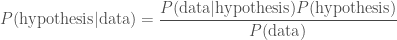
In this context, we give names to each of the probabilities (to make things sound extra fancy): $P(\mathrm{hypothesis}|\mathrm{data})$ is the posterior, because it’s what we get at the end; $P(\mathrm{data}|\mathrm{hypothesis})$ is the likelihood, it’s what you may remember calculating in statistics classes; $P(\mathrm{hypothesis})$ is the prior, because it’s what we believed about our hypothesis before we got the data, and $P(\mathrm{data})$ is the evidence. If ever you hear of someone doing something in a Bayesian way, it just means they are using the formula above. I think it’s rather silly to point this out, as it’s really the only logical way to do science, but people like to put “Bayesian” in the title of their papers as it sounds cool.

Whenever you get some new information, some new data, you should update your belief in your hypothesis using the above. The prior is what you believed about hypothesis before, and the posterior is what you believe after (you’ll use this posterior as your prior next time you learn something new). There are a couple of examples below, but before we get there I will take a moment to discuss priors.

About priors: what we already know

There have been many philosophical arguments about the use of priors in science. People worry that what you believe affects the results of science. Surely science should be above such things: it should be about truth, and should not be subjective! Sadly, this is not the case. Using Bayes’ theorem is the only logical thing to do. You can’t calculate a probability of what you believe after you get some data unless you know what you believed beforehand. If this makes you unhappy, just remember that when we changed our probability for it being raining outside, it didn’t change whether it was raining or not. If two different people use two different priors they can get two different results, but that’s OK, because they know different things, and so they should expect different things to happen.

To try to convince yourself that priors are necessary, consider the case that you are Sherlock Holmes (one of the modern versions), and you are trying to solve a bank robbery. There is a witness who saw the getaway, and they can remember what they saw with 99% accuracy (this gives the likelihood). If they say the getaway vehicle was a white transit van, do you believe them? What if they say it was a blue unicorn? In both cases the witness is the same, the likelihood is the same, but one is much more believable than the other. My prior that the getaway vehicle is a transit van is much greater than my prior for a blue unicorn: the latter can’t carry nearly as many bags of loot, and so is a silly choice.

If you find that changing your prior (to something else sensible) significantly changes your results, this just means that your data don’t tell you much. Imagine that you checked the weather forecast before leaving the office and it said “cloudy with 0–100% chance of precipitation”. You basically believe the same thing before and after. This really means that you need more (or better) data. I’ll talk about some good ways of calculating priors in the future.

Solving the inverse problem

Example 1: Doughnut allergy

We shall now attempt to use Bayes’ theorem to calculate some posterior probabilities. First, let’s consider a worrying situation. Imagine there is a rare genetic disease that makes you allergic to doughnuts. One in a million people have this disease, that only manifests later in life. You have tested positive. The test is 99% successful at detecting the disease if it is present, and returns a false positive (when you don’t have the disease) 1% of the time. How worried should you be? Let’s work out the probability of having the disease given that you tested positive

$\displaystyle P(\mathrm{allergy}|\mathrm{positive}) = \frac{P(\mathrm{positive}|\mathrm{allergy})P(\mathrm{allergy})}{P(\mathrm{positive})}$ .

Our prior for having the disease is given by how common it is, $P(\mathrm{allergy}) = 10^{-6}$ . The prior probability of not having the disease is $P(\mathrm{no\: allergy}) = 1 - P(\mathrm{allergy})$ . The likelihood of our positive result is $P(\mathrm{positive}|\mathrm{allergy}) = 0.99$ , which seems worrying. The evidence, the total probability of testing positive $P(\mathrm{positive})$ is found by adding the probability of a true positive and a false positive

$P(\mathrm{positive}) = P(\mathrm{positive}|\mathrm{allergy})P(\mathrm{allergy}) + P(\mathrm{positive}|\mathrm{no\: allergy})P(\mathrm{no\: allergy})$ .

The probability of a false positive is $P(\mathrm{positive}|\mathrm{no\: allergy}) = 0.01$ . We thus have everything we need. Substituting everything in, gives

$\displaystyle P(\mathrm{allergy}|\mathrm{positive}) = \frac{0.99 \times 10^{-6}}{0.99 \times 10^{-6} + 0.01 \times (1 - 10^{-6})} = 9.899 \times 10^{-5}$ .

Even after testing positive, you still only have about a one in ten thousand chance of having the allergy. While it is more likely that you have the allergy than a random member of the public, it’s still overwhelmingly probable that you’ll be fine continuing to eat doughnuts. Hurray!

Doughnut love: probably fine.

Example 2: Boys, girls and water balloons

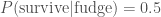
Second, imagine that Iris has three children. You know she has a boy and a girl, but you don’t know if she has two boys or two girls. You pop around for doughnuts one afternoon, and a girl opens the door. She is holding a large water balloon. What’s the probability that Iris has two girls? We want to calculate the posterior

$\displaystyle P(\mathrm{two\: girls}|\mathrm{girl\:at\:door}) = \frac{P(\mathrm{girl\:at\:door}|\mathrm{two\: girls})P(\mathrm{two\: girls})}{P(\mathrm{girl\:at\:door})}$ .

As a prior, we’d expect boys and girls to be equally common, so $P(\mathrm{two\: girls}) = P(\mathrm{two\: boys}) = 1/2$ . If we assume that it is equally likely that any one of the children opened the door, then the likelihood that one of the girls did so when their are two of them is $P(\mathrm{girl\:at\:door}|\mathrm{two\: girls}) = 2/3$ . Similarly, if there were two boys, the probability of a girl answering the door is $P(\mathrm{girl\:at\:door}|\mathrm{two\: boys}) = 1/3$ . The evidence, the total probability of a girl being at the door is

$P(\mathrm{girl\:at\:door}) =P(\mathrm{girl\:at\:door}|\mathrm{two\: girls})P(\mathrm{two\: girls}) +P(\mathrm{girl\:at\:door}|\mathrm{two\: boys}) P(\mathrm{two\: boys})$ .

Using all of these,

$\displaystyle P(\mathrm{two\: girls}|\mathrm{girl\:at\:door}) = \frac{(2/3)(1/2)}{(2/3)(1/2) + (1/3)(1/2)} = \frac{2}{3}$ .

Even though we already knew there was at least one girl, seeing a girl first makes it much more likely that the Iris has two daughters. Whether or not you end up soaked is a different question.

Example 3: Fudge!

Finally, we shall return to the case of Ted and his overconsumption of fudge. Ted claims to have eaten a lethal dose of fudge. Given that he is alive to tell the anecdote, what is the probability that he actually ate the fudge? Here, our data is that Ted is alive, and our hypothesis is that he did eat the fudge. We have

$\displaystyle P(\mathrm{fudge}|\mathrm{survive}) = \frac{P(\mathrm{survive}|\mathrm{fudge})P(\mathrm{fudge})}{P(\mathrm{survive})}$ .

This is a case where our prior, the probability that he would eat a lethal dose of fudge $P(\mathrm{fudge})$ , makes a difference. We know the probability of surviving the fatal dose is $P(\mathrm{survive}|\mathrm{fudge}) = 0.5$ . The evidence, the total probability of surviving $P(\mathrm{survive})$ , is calculated by considering the two possible sequence of events: either Ted ate the fudge and survived or he didn’t eat the fudge and survived

$P(\mathrm{survive}) = P(\mathrm{survive}|\mathrm{fudge})P(\mathrm{fudge}) + P(\mathrm{survive}|\mathrm{no\: fudge})P(\mathrm{no\: fudge})$ .

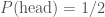
We’ll assume if he didn’t eat the fudge he is guaranteed to be alive, $P(\mathrm{survive}| \mathrm{no\: fudge}) = 1$ . Since Ted either ate the fudge or he didn’t $P(\mathrm{fudge}) + P(\mathrm{no\: fudge}) = 1$ . Therefore,

$P(\mathrm{survive}) = 0.5 P(\mathrm{fudge}) + [1 - P(\mathrm{fudge})] = 1 - 0.5 P(\mathrm{fudge})$ .

This gives us a posterior

$\displaystyle P(\mathrm{fudge}|\mathrm{survive}) = \frac{0.5 P(\mathrm{fudge})}{1 - 0.5 P(\mathrm{fudge})}$ .

We just need to decide on a suitable prior.

If we believe Ted could never possibly lie, then he must have eaten that fudge and $P(\mathrm{fudge}) = 1$ . In this case,

$\displaystyle P(\mathrm{fudge}|\mathrm{survive}) = \frac{0.5}{1 - 0.5} = 1$ .

Since we started being absolutely sure, we end up being absolutely sure: nothing could have changed our mind! This is a poor prior: it is too strong, we are being closed-minded. If you are closed-minded you can never learn anything new.

If we don’t know who Ted is, what fudge is, or the ease of consuming a lethal dose, then we might assume an equal prior on eating the fudge and not eating the fudge, $P(\mathrm{fudge}) = 0.5$ . In this case we are in a state of ignorance. Our posterior is

$\displaystyle P(\mathrm{fudge}|\mathrm{survive}) = \frac{0.5 \times 0.5}{1 - 0.5 \times 0.5} = \frac{1}{3}$ .

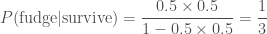
Even though we know nothing, we conclude that it’s more probable that the Ted did not eat the fudge. In fact, it’s twice as probable that he didn’t eat the fudge than he did as $P(\mathrm{no\: fudge}|\mathrm{survive}) = 1 -P(\mathrm{fudge}|\mathrm{survive}) = 2/3$ .

In reality, I think that it’s extremely improbable anyone could consume a lethal dose of fudge. I’m fairly certain that your body tries to protect you from such stupidity by expelling the fudge from your system before such a point. However, I will concede that it is not impossible. I want to assign a small probability to $P(\mathrm{fudge})$ . I don’t know if this should be one in a thousand, one in a million or one in a billion, but let’s just say it is some small value $p$ . Then

$\displaystyle P(\mathrm{fudge}|\mathrm{survive}) = \frac{0.5 p}{1 - 0.5 p} \approx 0.5 p$ .

as the denominator is approximately one. Whatever small probability I pick, it is half as probable that Ted ate the fudge.

I would assign a much higher probability to Mr. Impossible being able to eat that much fudge than Ted.

While it might not be too satisfying that we can’t come up with incontrovertible proof that Ted didn’t eat the fudge, we might be able to shut him up by telling him that even someone who knows nothing would think his story is unlikely, and that we will need much stronger evidence before we can overcome our prior.

Homework example: Monty Hall

You now have all the tools necessary to tackle the Monty Hall problem, one of the most famous probability puzzles:

You are on a game show and are given the choice of three doors. Behind one is a car (a Lincoln Continental), but behind the others are goats (which you don’t want). You pick a door. The host, who knows what is behind the doors, opens another door to reveal goat. They then offer you the chance to switch doors. Should you stick with your current door or not? — Monty Hall problem

You should be able to work out the probability of winning the prize by switching and sticking. You can’t guarantee you win, but you can maximise your chances.

Summary

Whenever you encounter new evidence, you should revise how probable you think things are. This is true in science, where we perform experiments to test hypotheses; it is true when trying to solve a mystery using evidence, or trying to avoid getting a goat on a game show. Bayes’ theorem is used to update probabilities. Although Bayes’ theorem itself is quite simple, calculating likelihoods, priors and evidences for use in it can be difficult. I hope to return to all these topics in the future.

An introduction to probability: Leaving nothing to chance

August 9, 2014October 25, 2014 / CPLB / Leave a comment

Probabilities and science

Understanding probabilities is important in science. Once you’ve done an experiment, you need to be able to extract from your data information about your theory. Only rarely do you get a simple yes or no: most of the time you have to work with probabilities to quantify your degree of certainty. I’ll (probably) be writing about probabilities in connection with my research, so I thought it would be useful to introduce some of the concepts.

I’ll be writing a series of posts, hopefully going through from the basics to the limits of my understanding. We’ll begin with introducing the concept of probability. There’s a little bit of calculus, but you can skip that without effecting the rest, just remember you can’t grow up to be big and strong if you don’t finish your calculus.

What is a probability?

A probability describes the degree of belief that you have in a proposition. We talk about probabilities quite intuitively: there are some angry-looking, dark clouds overhead and I’ve just lit the barbecue, so it’s probably going to rain; it’s more likely that United will win this year’s sportsball league than Rovers, or it’s more credible that Ted is exaggerating in his anecdote than he actually ate that much fudge…

We formalise the concept of a probability, so that it can be used in calculations, by assigning them numerical values (not by making them wear a bow-tie, although that is obviously cool). Conventionally, we use 0 for impossible, 1 for certain and the range in between for intermediate probabilities. For example, if we were tossing a coin, we might expect it to be heads half the time, hence the probability of heads is $P(\mathrm{head}) = 1/2$ , or if rolling a die, the probability of getting a six is $P(6) = 1/6$ .

For both the coin and the die we have a number of equally probable outcomes: two for the coin (heads and tails) and six for the die (1, 2, 3, 4, 5 and 6). This does not have to be the case: imagine picking a letter at random from a sample of English text. Some letters are more common than others—this is why different letters have different values in Scrabble and why hangman can be tricky. The most frequent letter is “e”, the probability of picking it is about 0.12, and the least frequent is “z”, the probability of picking that is just 0.0007.

Often we consider a parameter that has a continuous range, rather than discrete values (as in the previous examples). For example, I might be interested in the mass of a black hole, which can have any positive value. We then use a probability density function $p(x)$ such that the probability for the parameter lies in the range $a \leq x \leq b$ is given by the integral

$\displaystyle P(a \leq x \leq b) = \int_a^b p(x)\, \mathrm{d}x$ .

Performing an integral is just calculating the area under a curve, it can be thought of a the equivalent of adding up an infinite number of infinitely closely spaced slices. Returning to how much fudge Ted actually ate, we might to find the probability that he a mass of fudge $m$ that was larger than zero, but smaller than the fatal dose $M$ . If we a had probability density function $p(m)$ , we would calculate

$\displaystyle P(0 < m \leq M) = \int_0^{M} p(m)\, \mathrm{d}m$ .

The probability density is largest where the probability is greatest and smallest where the probability is smallest, as you’d expect. Calculating probabilities and probability distributions is, in general, a difficult problem, it’s actually what I spend a lot of my time doing. We’ll return to calculating probabilities later.

Combining probabilities

There are several recipes for combining probabilities to construct other probabilities, just like there are recipes to combine sugar and dairy to make fudge. Admittedly, probabilities are less delicious than fudge, but they are also less likely to give you cavities. If we have a set of of disjoint outcomes, we can work out the probability of that set by adding up the probabilities of the individual outcomes. For example, when rolling our die, the probability of getting an even number is

$\displaystyle P(\mathrm{even}) = P(2) + P(4) + P(6) = \frac{1}{6} +\frac{1}{6} +\frac{1}{6} = \frac{1}{2}$ .

(This is similar to what we’re doing when integrating up the probability density function for continuous distributions: there we’re adding up the probability that the variable $x$ is in each infinitesimal range $\mathrm{d}x$ ).

If we have two independent events, then the probability of both of them occurring is calculated by multiplying the two individual probabilities together. For example, we could consider the probability of rolling a six and the probability of Ted surviving eating the lethal dose of fudge, then

$\displaystyle P(\mathrm{6\: and\: survive}) = P(6) \times P(\mathrm{survive})$ .

The most commonly quoted quantity for a lethal dose is the median lethal dose or LD₅₀, which is the dose that kills half the population, so we can take the probability of surviving to be 0.5. Thus,

$\displaystyle P(\mathrm{6\: and\: survive}) = P(6) \times P(\mathrm{survive}) = \frac{1}{12}$ .

Events are independent if they don’t influence each other. Rolling a six shouldn’t influence Ted’s medical condition, and Ted’s survival shouldn’t influence the roll of a die, so these events are independent.

Things are more interesting when events are not independent. We then have to deal with conditional probabilities: the conditional probability $P(\mathrm{A}|\mathrm{B})$ is the probability of $\mathrm{A}$ given that $B$ is true. For example, if I told you that I rolled an even number, the probability of me having rolled a six is $P(6|\mathrm{even}) = 1/3$ . If I told you that I have rolled a six, then the probability of me having rolled an even number is $P(\mathrm{even}|6) = 1$ —it’s a dead cert, so bet all your fudge on that! When combining probabilities from dependent events, we chain probabilities together in a logical chain. The probability of rolling a six and an even number is the probability of rolling an even number multiplied by the probability of rolling a six given that I rolled an even number

$\displaystyle P(\mathrm{6\: and\: even}) = P(6|\mathrm{even}) \times P(\mathrm{even})= \frac{1}{3} \times \frac{1}{2} = \frac{1}{6}$ ,

or equivalently the probability of rolling six multplied by the probability of rolling an even number given that I rolled a six

$\displaystyle P(\mathrm{6\: and\: even}) = P(\mathrm{even} | 6) \times P(6) = 1 \times \frac{1}{6} = \frac{1}{6}$ .

Reassuringly, we do get the same answer. This is a bit of a silly example, as we know that if we’ve rolled a six we have rolled an even number, so all we are doing if calculating the probability of rolling a six.

We can use conditional probabilities for independent events: this is really easy as the conditional probability is just the straight probability. The probability of Ted surviving his surfeit of fudge given that I rolled a six is just the probability of him surviving, $P(\mathrm{survive}|6) = P(\mathrm{survive})$ .

Let’s try a more complicated example, let’s imagine that Ted is playing fudge roulette. This is like Russian roulette, except you roll a die and if it comes up six, then you have to eat the lethal dose of fudge. His survival probability now depends on the roll of the die. We want to calculate the probability that Ted will live to tomorrow. If Ted doesn’t roll a six, we’ll assume that he has a 100% survive rate (based on that one anecdote where he claims to have created a philosopher’s stone by soaking duct tape in holy water), this isn’t quite right, but is good enough. The probability of Ted surviving given he didn’t roll a six is

$\displaystyle P(\mathrm{not\: 6\: and\: survive}) = P(\mathrm{survive} | \mathrm{not\: 6}) \times P(\mathrm{not\: 6}) = 1 \times \frac{5}{6} = \frac{5}{6}$ .

The probability of Ted rolling a six (and eating the fudge) and then surviving is

$\displaystyle P(\mathrm{6\: and\: survive}) = P(\mathrm{survive} | \mathrm{6}) \times P(\mathrm{6}) = \frac{1}{2} \times \frac{1}{6} = \frac{1}{12}$ .

We have two disjoint outcomes (rolling a six and survivng, and not rolling a six and surving), so the total probability of surviving is given by the sum

$\displaystyle P(\mathrm{survive}) =P(\mathrm{not\: 6\: and\: survive}) +P(\mathrm{6\: and\: survive}) = \frac{5}{6} +\frac{1}{12} =\frac{11}{12}$ .

It seems likely that he’ll make it, although fudge roulette is still a dangerous game!

There’s actually an easier way of calculating the probability that Ted survives. There are only two possible outcomes: Ted survives or he doesn’t. Since one of these must happen, their probabilities must add to one: the survive probability is

$P(\mathrm{survive}) = 1 - P(\mathrm{not\: survive})$ .

We’ve already seen this, as we’ve used the probability of not rolling a six is $P(\mathrm{not\: 6}) = 1 - P(6) = 5/6$ . The probability of not surviving is much easier to work out as there’s only one way that can happen: rolling a six and then overdosing on fudge. The probability is

$\displaystyle P(\mathrm{not\: surviving}) = P(\mathrm{fudge\: overdose}|6) \times P(6) = \frac{1}{2} \times \frac{1}{6} = \frac{1}{12}$ ,

and so the survival probability is $P(\mathrm{survive}) = 1 - 1/12 = 11/12$ , exactly as before, but in fewer steps.

In a future post we’ll try working out the probability that Ted did eat a lethal dose of fudge given that he is alive to tell the anecdote. This is known as an inverse problem, and is similar to what scientists do all the time. We do experiments and get data, then we need to work out the probability of our theory (that Ted ate the fudge) being correct given the data (that he’s still alive).

Interpreting probabilities

We have now discussed what a probability is and how we can combine them. We should now think about how to interpret them. It’s easy enough to understand that a probability of 0.05 means that we expect something should happen on average once in 20 times, and that it is more probable than something with a probability of 0.01, but less likely than something with a probability of 0.10. However, we are not good at having an intuitive understanding of probabilities.

Consider the case that a scientist announces a result with 95% confidence. That sounds pretty good. Think how surprised you would be (assuming that their statistics are all correct) that the result was wrong. I feel like I would be pretty surprised. Now consider rolling tow dice, how surprised would you be if you rolled two sixes? The probability of the result being wrong is $1 - 0.95 = 0.05$ , or one in twenty. The probability of rolling two sixes is $1/6 \times 1/6 = 1/36$ or about one in forty. Hence, you should be almost twice as surprised by rolling double six as for a 95% confidence-level result being incorrect.

When dealing with probabilities, I find it useful to make a comparison to something familiar. While Ted is more likely than not to survive fudge roulette, there is a one is twelve chance of dying. That’s three times as likely as rolling a double six, or equally probable as rolling a six and getting heads. That’s riskier than I’d like, so I’m going to stick to consuming fudge in moderation.

Christopher Berry

Gravitational-wave astronomer

fudge

An introduction to probability: Inference and learning from data

Taking an umbrella

Bayes’ theorem

About priors: what we already know