Gravity Spy is an awesome project that combines citizen science and machine learning to classify glitches in LIGO and Virgo data. Glitches are short bursts of noise in our detectors which make analysing our data more difficult. Some glitches have known causes, others are more mysterious. Classifying glitches into different types helps us better understand their properties, and in some cases track down their causes and eliminate them! In this paper, led by Scotty Coughlin, we demonstrated the effectiveness of a new tool which are citizen scientists can use to identify new glitch classes.
The Gravity Spy project
Gravitational-wave detectors are complicated machines. It takes a lot of engineering to achieve the required accuracy needed to observe gravitational waves. Most of the time, our detectors perform well. The background noise in our detectors is easy to understand and model. However, our detectors are also subject to glitches, unusual (sometimes extremely loud and complicated) noise that doesn’t fit the usual properties of noise. Glitches are short, they only appear in a small fraction of the total data, but they are common. This makes detection and analysis of gravitational-wave signals more difficult. Detection is tricky because you need to be careful to distinguish glitches from signals (and possibly glitches and signals together), and understanding the signal is complicated as we may need to model a signal and a glitch together [bonus note]. Understanding glitches is essential if gravitational-wave astronomy is to be a success.
To understand glitches, we need to be able to classify them. We can search for glitches by looking for loud pops, whooshes and splats in our data. The task is then to spot similarities between them. Once we have a set of glitches of the same type, we can examine the state of the instruments at these times. In the best cases, we can identify the cause, and then work to improve the detectors so that this no longer happens. Other times, we might be able to find the source, but we can find one of the monitors in our detectors which acts a witness to the glitch. Then we know that if something appears in that monitor, we expect a glitch of a particular form. This might mean that we throw away that bit of data, or perhaps we can use the witness data to subtract out the glitch. Since glitches are so common, classifying them is a huge amount of work. It is too much for our detector characterisation experts to do by hand.
There are two cunning options for classifying large numbers of glitches
Get a computer to do it. The difficulty is teaching a computer to identify the different classes. Machine-learning algorithms can do this, if they are properly trained. Training can require a large training set, and careful validation, so the process is still labour intensive.
Get lots of people to help. The difficulty here is getting non-experts up-to-speed on what to look for, and then checking that they are doing a good job. Crowdsourcing classifications is something citizen scientists can do, but we will need a large number of dedicated volunteers to tackle the full set of data.
The idea behind Gravity Spy is to combine the two approaches. We start with a small training set from our detector characterization experts, and train a machine-learning algorithm on them. We then ask citizen scientists (thanks Zooniverse) to classify the glitches. We start them off with glitches the machine-learning algorithm is confident in its classification; these should be easy to identify. As citizen scientists get more experienced, they level up and start tackling more difficult glitches. The citizen scientists validate the classifications of the machine-learning algorithm, and provide a larger training set (especially helpful for the rarer glitch classes) for it. We can then happily apply the machine-learning algorithm to classify the full data set [bonus note].
How Gravity Spy works: the interconnection of machine-learning classification and citizen-scientist classification. The similarity search is used to identify glitches similar to one which do not fit into current classes. Figure 2 of Coughlin et al. (2019).
I especially like the levelling-up system in Gravity Spy. I think it helps keep citizen scientists motivated, as it both prevents them from being overwhelmed when they start and helps them see their own progress. I am currently Level 4.
Gravity Spy works using images of the data. We show spectrograms, plots of how loud the output of the detectors are at different frequencies at different times. A gravitational wave form a binary would show a chirp structure, starting at lower frequencies and sweeping up.
Spectrogram showing the upward-sweeping chirp of gravitational wave GW170104 as seen in Gravity Spy. I correctly classified this as a Chirp.
New glitches
The Gravity Spy system works smoothly. However, it is set up to work with a fixed set of glitch classes. We may be missing new glitch classes, either because they are rare, and hadn’t been spotted by our detector characterization team, or because we changed something in our detectors and new class arose (we expect this to happen as we tune up the detectors between observing runs). We can add more classes to our citizen scientists and machine-learning algorithm to use, but how do we spot new classes in the first place?
Our citizen scientists managed to identify a few new glitches by spotting things which didn’t fit into any of the classes. These get put in the None-of-the-Above class. Occasionally, you’ll come across similar looking glitches, and by collecting a few of these together, build a new class. The Paired Dove and Helix classes were identified early on by our citizen scientists this way; my favourite suggested new class is the Falcon [bonus note]. The difficulty is finding a large number of examples of a new class—you might only recognise a common feature after going past a few examples, backtracking to find the previous examples is hard, and you just have to keep working until you are lucky enough to be given more of the same.
Example Helix (left) and Paired Dove glitches. These classes were identified by Gravity Spy citizen scientists. Helix glitches are related to related to hiccups in the auxiliary lasers used to calibrate the detectors by pushing on the mirrors. Paired Dove glitches are related to motion of the beamsplitter in the interferometer. Adapted from Figure 8 of Zevin et al. (2017).
To help our citizen scientists find new glitches, we created a similar search. Having found an interesting glitch, you can search for similar examples, and put quickly put together a collection of your new class. The video below shows how it works. The thing we had to work out was how to define similar?
Transfer learning
Our machine-learning algorithm only knows about the classes we tell it about. It then works out the features we distinguish the different classes, and are common to glitches of the same class. Working in this feature space, glitches form clusters of different classes.
Visualisation showing the clustering of different glitches in the Gravity Spy feature space. Each point is a different glitch from our training set. The feature space has more than three dimensions: this visualisation was made using a technique which preserves the separation and clustering of different and similar points. Figure 1 of Coughlin et al. (2019).
For our similarity search, our idea was to measure distances in feature space [bonus note for experts]. This should work well if our current set of classes have a wide enough set of features to capture to characteristics of the new class; however, it won’t be effective if the new class is completely different, so that its unique features are not recognised. As an analogy, imagine that you had an algorithm which classified M&M’s by colour. It would probably do well if you asked it to distinguish a new colour, but would probably do poorly if you asked it to distinguish peanut butter filled M&M’s as they are identified by flavour, which is not a feature it knows about. The strategy of using what a machine learning algorithm learnt about one problem to tackle a new problem is known as transfer learning, and we found this strategy worked well for our similarity search.
Raven Pecks and Water Jets
To test our similarity search, we applied it to two glitches classes not in the Gravity Spy set:
Raven Peck glitches are caused by thirsty ravens pecking ice built up along nitrogen vent lines outside of the Hanford detector. Raven Pecks look like horizontal lines in spectrograms, similar to other Gravity Spy glitch classes (like the Power Line, Low Frequency Line and 1080 Line). The similarity search should therefore do a good job, as we should be able to recognise its important features.
Water Jet glitches were caused by local seismic noise at the Hanford detector which causes loud bands which disturb the input laser optics. These glitches are found between , over which time there are 26,871 total glitches in GRavity Spy. The Water Jet glitch doesn’t have anything to do with water, it is named based on its appearance (like a fountain, not a weasel). Its features are subtle, and unlike other classes, so we would expect this to be difficult for our similarity search to handle.
These glitches appeared in the data from the second observing run. Raven Pecks appeared between 14 April and 9 August 2017, and Water Jets appeared 4 January and 28 May 2017. Over these intervals there are a total of 13,513 and 26,871 Gravity Spy glitches from all type, so even if you knew exactly when to look, you have a large number to search through to find examples.
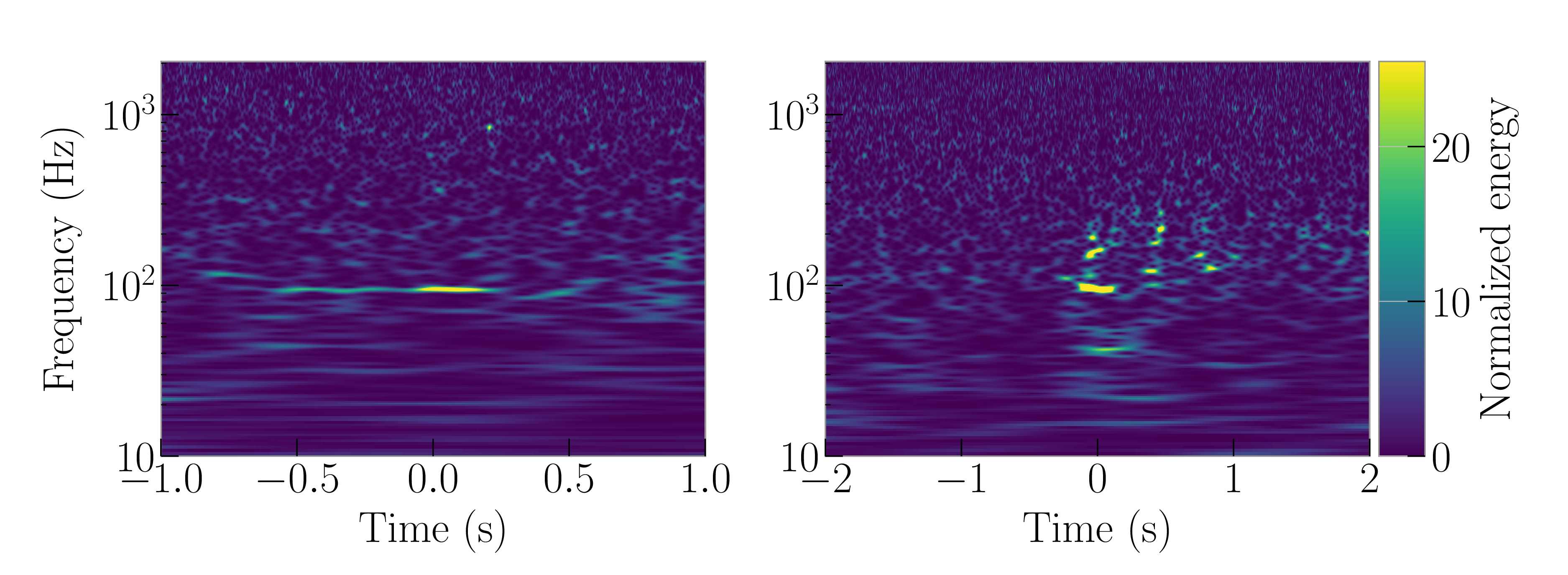
Example Raven Peck (left) and Water Jet (right) glitches. These classes of glitch are not included in the usual Gravity Spy scheme. Adapted from Figure 3 of Coughlin et al. (2019).
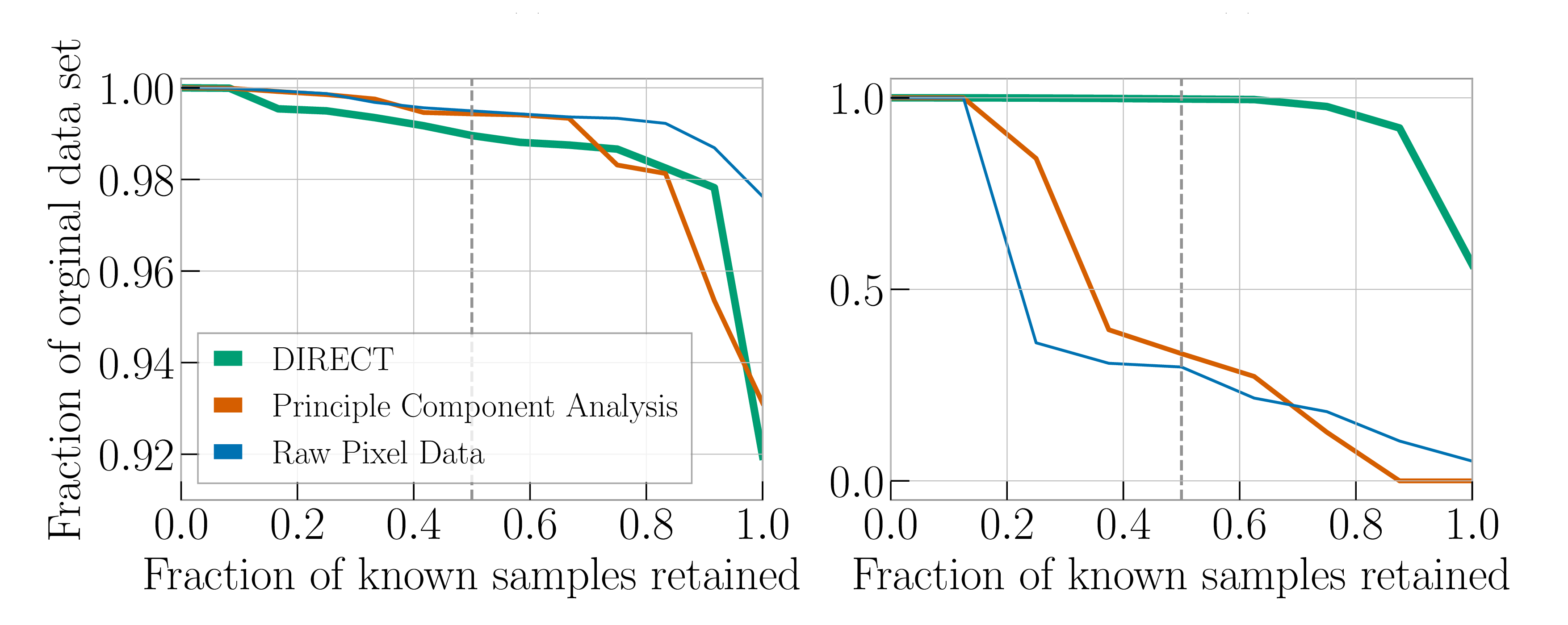
We tested using our machine-learning feature space for the similarity search against simpler approaches: using the raw difference in pixels, and using a principal component analysis to create a feature space. Results are shown in the plots below. These show the fraction of glitches we want returned by the similarity search versus the total number of glitches rejected. Ideally, we would want to reject all the glitches except the ones we want, so the search would return 100% of the wanted classes and reject almost 100% of the total set. However, the actual results will depend on the adopted threshold for the similarity search: if we’re very strict we’ll reject pretty much everything, and only get the most similar glitches of the class we want, if we are too accepting, we get everything back, regardless of class. The plots can be read as increasing the range of the similarity search (becoming less strict) as you go left to right.
Performance of the similarity search for Raven Peck (left) and Water Jet (right) glitches: the fraction of known glitches of the desired class that have a higher similarity score (compared to an example of that glitch class) than a given percentage of full data set. Results are shown for three different ways of defining similarity: the DIRECT machine-learning algorithm feature space (think line), a principal component analysis (medium line) and a comparison of pixels (thin line). Adapted from Figure 3 of Coughlin et al. (2019).
For the Raven Peck, the similarity search always performs well. We have 50% of Raven Pecks returned while rejecting 99% of the total set of glitches, and we can get the full set while rejecting 92% of the total set! The performance is pretty similar between the different ways of defining feature space. Raven Pecks are easy to spot.
Water Jets are more difficult. When we have 50% of Water Jets returned by the search, our machine-learning feature space can still reject almost all glitches. The simpler approaches do much worse, and will only reject about 30% of the full data set. To get the full set of Water Jets we would need to loosen the similarity search so that it only rejects 55% of the full set using our machine-learning feature space; for the simpler approaches we’d basically get the full set of glitches back. They do not do a good job at narrowing down the hunt for glitches. Despite our suspicion that our machine-learning approach would struggle, it still seems to do a decent job [bonus note for experts].
Do try this at home
Having developed and testing our similarity search tool, it is now live. Citizen scientists can use it to hunt down new glitch classes. Several new glitches classes have been identified in data from LIGO and Virgo’s (currently ongoing) third observing run. If you are looking for a new project, why not give it a go yourself? (Or get your students to give it a go, I’ve had some reasonable results with high-schoolers). There is the real possibility that your work could help us with the next big gravitational-wave discovery.
The best example of a gravitational-wave overlapping a glitch is GW170817. The glitch meant that the signal in the LIGO Livingston detector wasn’t immediately recognised. Fortunately, the signal in the Hanford detector was easy to spot. The glitch was analyse and categorised in Gravity Spy. It is a simple glitch, so it wasn’t too difficult to remove from the data. As our detectors become more sensitive, so that detections become more frequent, we expect that signal overlapping with glitches will become a more common occurrence. Unless we can eliminate glitches, it is only a matter of time before we get a glitch that prevents us from analysing an important signal.
Gravitational-wave alerts
In the third observing run of LIGO and Virgo, we send out automated alerts when we have a new gravitational-wave candidate. Astronomers can then pounce into action to see if they can spot anything coinciding with the source. It is important to quickly check the state of the instruments to ensure we don’t have a false alarm. To help with this, a data quality report is automatically prepared, containing many diagnostics. The classification from the Gravity Spy algorithm is one of many pieces of information included. It is the one I check first.
The Falcon
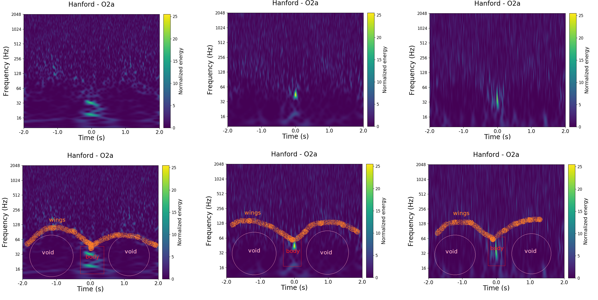
Excellent Gravity Spy moderator EcceruElme suggested a new glitch class Falcon. This suggestion was followed up by Oli Patane, they found that all the examples identified occured between 6:30 am and 8:30 am on 20 June 2017 in the Hanford detector. The instrument was misbehaving at the time. To solve this, the detector was taken out of observing mode and relocked (the equivalent of switching it off and on again). Since this glitch class was only found in this one 2-hour window, we’ve not added it as a class. I love how it was possible to identify this problematic stretch of time using only Gravity Spy images (which don’t identify when they are from). I think this could be the seed of a good detective story. The Hanfordese Falcon?
Examples of the proposed Falcon glitch class, illustrating the key features (and where the name comes from). This new glitch class was suggested by Gravity Spy citizen scientist EcceruElme.
Distance measure
We chose a cosine distance to measure similarity in feature space. We found this worked better than a Euclidean metric. Possibly because for identifying classes it is more important to have the right mix of features, rather than how significant the individual features are. However, we didn’t do a systematic investigation of the optimal means of measuring similarity.
Retraining the neural net
We tested the performance of the machine-learning feature space in the similarity search after modifying properties of our machine-learning algorithm. The algorithm we are using is a deep multiview convolution neural net. We switched the activation function in the fully connected layer of the net, trying tanh and leaukyREU. We also varied the number of training rounds and the number of pairs of similar and dissimilar images that are drawn from the training set each round. We found that there was little variation in results. We found that leakyREU performed a little better than tanh, possibly because it covers a larger dynamic range, and so can allow for cleaner separation of similar and dissimilar features. The number of training rounds and pairs makes negligible difference, possibly because the classes are sufficiently distinct that you don’t need many inputs to identify the basic features to tell them apart. Overall, our results appear robust. The machine-learning approach works well for the similarity search.
On 4 January 2017, Advanced LIGO made a new detection of gravitational waves. The signal, which we call GW170104 [bonus note], came from the coalescence of two black holes, which inspiralled together (making that characteristic chirp) and then merged to form a single black hole.
On 4 January 2017, I was just getting up off the sofa when my phone buzzed. My new year’s resolution was to go for a walk every day, and I wanted to make use of the little available sunlight. However, my phone informed me that PyCBC (one or our search algorithms for signals from coalescing binaries) had identified an interesting event. I sat back down. I was on the rota to analyse interesting signals to infer their properties, and I was pretty sure that people would be eager to see results. They were. I didn’t leave the sofa for the rest of the day, bringing my new year’s resolution to a premature end.
Since 4 January, my time has been dominated by working on GW170104 (you might have noticed a lack of blog posts). Below I’ll share some of my war stories from life on the front line of gravitational-wave astronomy, and then go through some of the science we’ve learnt. (Feel free to skip straight to the science, recounting the story was more therapy for me).
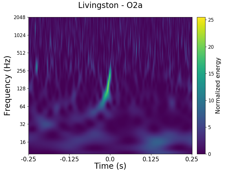
Time–frequency plots for GW170104 as measured by Hanford (top) and Livingston (bottom). The signal is clearly visible as the upward sweeping chirp. The loudest frequency is something between E3 and G♯3 on a piano, and it tails off somewhere between D♯4/E♭4 and F♯4/G♭4. Part of Fig. 1 of the GW170104 Discovery Paper.
The story
In the second observing run, the Parameter Estimation group have divided up responsibility for analysing signals into two week shifts. For each rota shift, there is an expert and a rookie. I had assumed that the first slot of 2017 would be a quiet time. The detectors were offline over the holidays, due back online on 4 January, but the instrumentalists would probably find some extra tinkering they’d want to do, so it’d probably slip a day, and then the weather would be bad, so we’d probably not collect much data anyway… I was wrong. Very wrong. The detectors came back online on time, and there was a beautifully clean detection on day one.
My partner for the rota was Aaron Zimmerman. 4 January was his first day running parameter estimation on live signals. I think I would’ve run and hidden underneath my duvet in his case (I almost did anyway, and I lived through the madness of our first detection GW150914), but he rose to the occasion. We had first results after just a few hours, and managed to send out a preliminary sky localization to our astronomer partners on 6 January. I think this was especially impressive as there were some difficulties with the initial calibration of the data. This isn’t a problem for the detection pipelines, but does impact the parameters which we infer, particularly the sky location. The Calibration group worked quickly, and produced two updates to the calibration. We therefore had three different sets of results (one per calibration) by 6 January [bonus note]!
Producing the final results for the paper was slightly more relaxed. Aaron and I conscripted volunteers to help run all the various permutations of the analysis we wanted to double-check our results [bonus note].
Recovered gravitational waveforms from analysis of GW170104. The broader orange band shows our estimate for the waveform without assuming a particular source (wavelet). The narrow blue bands show results if we assume it is a binary black hole (BBH) as predicted by general relativity. The two match nicely, showing no evidence for any extra features not included in the binary black hole models. Figure 4 of the GW170104 Discovery Paper.
I started working on GW170104 through my parameter estimation duties, and continued with paper writing.
Ahead of the second observing run, we decided to assemble a team to rapidly write up any interesting binary detections, and I was recruited for this (I think partially because I’m not too bad at writing and partially because I was in the office next to John Veitch, one of the chairs of the Compact Binary Coalescence group,so he can come and check that I wasn’t just goofing off eating doughnuts). We soon decided that we should write a paper about GW170104, and you can decide whether or not we succeeded in doing this rapidly…
Being on the paper writing team has given me huge respect for the teams who led the GW150914 and GW151226 papers. It is undoubtedly one of the most difficult things I’ve ever done. It is extremely hard to absorb negative remarks about your work continuously for months [bonus note]—of course people don’t normally send comments about things that they like, but that doesn’t cheer you up when you’re staring at an inbox full of problems that need fixing. Getting a collaboration of 1000 people to agree on a paper is like herding cats while being a small duckling.
On of the first challenges for the paper writing team was deciding what was interesting about GW170104. It was another binary black hole coalescence—aren’t people getting bored of them by now? The signal was quieter than GW150914, so it wasn’t as remarkable. However, its properties were broadly similar. It was suggested that perhaps we should title the paper “GW170104: The most boring gravitational-wave detection”.
One potentially interesting aspect was that GW170104 probably comes from greater distance than GW150914 or GW151226 (but perhaps not LVT151012) [bonus note]. This might make it a good candidate for testing for dispersion of gravitational waves.
Dispersion occurs when different frequencies of gravitational waves travel at different speeds. A similar thing happens for light when travelling through some materials, which leads to prisms splitting light into a spectrum (and hence the creation of Pink Floyd album covers). Gravitational waves don’t suffered dispersion in general relativity, but do in some modified theories of gravity.
It should be easier to spot dispersion in signals which have travelled a greater distance, as the different frequencies have had more time to separate out. Hence, GW170104 looks pretty exciting. However, being further away also makes the signal quieter, and so there is more uncertainty in measurements and it is more difficult to tell if there is any dispersion. Dispersion is also easier to spot if you have a larger spread of frequencies, as then there can be more spreading between the highest and lowest frequencies. When you throw distance, loudness and frequency range into the mix, GW170104 doesn’t always come out on top, depending upon the particular model for dispersion: sometimes GW150914’s loudness wins, other times GW151226’s broader frequency range wins. GW170104 isn’t too special here either.
Even though GW170104 didn’t look too exciting, we started work on a paper, thinking that we would just have a short letter describing our observations. The Compact Binary Coalescence group decided that we only wanted a single paper, and we wouldn’t bother with companion papers as we did for GW150914. As we started work, and dug further into our results, we realised that actually there was rather a lot that we could say.
I guess the moral of the story is that even though you might be overshadowed by the achievements of your siblings, it doesn’t mean that you’re not awesome. There might not be one outstanding feature of GW170104, but there are lots of little things that make it interesting. We are still at the beginning of understanding the properties of binary black holes, and each new detection adds a little more to our picture.
I think GW170104 is rather neat, and I hope you do too.
As we delved into the details of our results, we realised there was actually a lot of things that we could say about GW170104, especially when considered with our previous observations. We ended up having to move some of the technical details and results to Supplemental Material. With hindsight, perhaps it would have been better to have a companion paper or two. However, I rather like how packed with science this paper is.
The paper, which Physical Review Letters have kindly accommodated, despite its length, might not be as polished a classic as the GW150914 Discovery Paper, but I think they are trying to do different things. I rarely ever refer to the GW150914 Discovery Paper for results (more commonly I use it for references), whereas I think I’ll open up the GW170104 Discovery Paper frequently to look up numbers.
Although perhaps not right away, I’d quite like some time off first. The weather’s much better now, perfect for walking…
Advanced LIGO’s first observing run was hugely successful. Running from 12 September 2015 until 19 January 2016, there were two clear gravitational-wave detections, GW1501914 and GW151226, as well as a less certain candidate signal LVT151012. All three (assuming that they are astrophysical signals) correspond to the coalescence of binary black holes.
The second observing run started 30 November 2016. Following the first observing run’s detections, we expected more binary black hole detections. On 4 January, after we had collected almost 6 days’ worth of coincident data from the two LIGO instruments [bonus note], there was a detection.
The searches
The signal was first spotted by an online analysis. Our offline analysis of the data (using refined calibration and extra information about data quality) showed that the signal, GW170104, is highly significant. For both GstLAL and PyCBC, search algorithms which use templates to search for binary signals, the false alarm rate is estimated to be about 1 per 70,000 years.
The signal is also found in unmodelled (burst) searches, which look for generic, short gravitational wave signals. Since these are looking for more general signals than just binary coalescences, the significance associated with GW170104 isn’t as great, and coherent WaveBurst estimates a false alarm rate of 1 per 20,000 years. This is still pretty good! Reconstructions of the waveform from unmodelled analyses also match the form expected for binary black hole signals.
The search false alarm rates are the rate at which you’d expect something this signal-like (or more signal-like) due to random chance, if you data only contained noise and no signals. Using our knowledge of the search pipelines, and folding in some assumptions about the properties of binary black holes, we can calculate a probability that GW170104 is a real astrophysical signal. This comes out to be greater than .
The source
As for the previous gravitational wave detections, GW170104 comes from a binary black hole coalescence. The initial black holes were and (where is the mass of our Sun), and the final black hole was . The quoted values are the median values and the error bars denote the central 90% probable range. The plot below shows the probability distribution for the masses; GW170104 neatly nestles in amongst the other events.
Estimated masses for the two black holes in the binary . The two-dimensional shows the probability distribution for GW170104 as well as 50% and 90% contours for all events. The one-dimensional plot shows results using different waveform models. The dotted lines mark the edge of our 90% probability intervals. Figure 2 of the GW170104 Discovery Paper.
GW150914 was the first time that we had observed stellar-mass black holes with masses greater than around . GW170104 has similar masses, showing that our first detection was not a fluke, but there really is a population of black holes with masses stretching up into this range.
Black holes have two important properties: mass and spin. We have good measurements on the masses of the two initial black holes, but not the spins. The sensitivity of the form of the gravitational wave to spins can be described by two effective spin parameters, which are mass-weighted combinations of the individual spins.
The effective inspiral spin parameter qualifies the impact of the spins on the rate of inspiral, and where the binary plunges together to merge. It ranges from +1, meaning both black holes are spinning as fast as possible and rotate in the same direction as the orbital motion, to −1, both black holes spinning as fast as possible but in the opposite direction to the way that the binary is orbiting. A value of 0 for could mean that the black holes are not spinning, that their rotation axes are in the orbital plane (instead of aligned with the orbital angular momentum), or that one black hole is aligned with the orbital motion and the other is antialigned, so that their effects cancel out.
The effective precession spin parameter qualifies the amount of precession, the way that the orbital plane and black hole spins wobble when they are not aligned. It is 0 for no precession, and 1 for maximal precession.
We can place some constraints on , but can say nothing about . The inferred value of the effective inspiral spin parameter is . Therefore, we disfavour large spins aligned with the orbital angular momentum, but are consistent with small aligned spins, misaligned spins, or spins antialigned with the angular momentum. The value is similar to that for GW150914, which also had a near-zero, but slightly negative of .
Estimated effective inspiral spin parameter and effective precession spin parameter. The two-dimensional shows the probability distribution for GW170104 as well as 50% and 90% contours. The one-dimensional plot shows results using different waveform models, as well as the prior probability distribution. The dotted lines mark the edge of our 90% probability intervals. We learn basically nothing about precession. Part of Figure 3 of the GW170104 Discovery Paper.
Converting the information about , the lack of information about , and our measurement of the ratio of the two black hole masses, into probability distributions for the component spins gives the plots below [bonus note]. We disfavour (but don’t exclude) spins aligned with the orbital angular momentum, but can’t say much else.
Estimated orientation and magnitude of the two component spins. The distribution for the more massive black hole is on the left, and for the smaller black hole on the right. The probability is binned into areas which have uniform prior probabilities, so if we had learnt nothing, the plot would be uniform. Part of Figure 3 of the GW170104 Discovery Paper.
One of the comments we had on a draft of the paper was that we weren’t making any definite statements about the spins—we would have if we could, but we can’t for GW170104, at least for the spins of the two inspiralling black holes. We can be more definite about the spin of the final black hole. If two similar mass black holes spiral together, the angular momentum from the orbit is enough to give a spin of around . The spins of the component black holes are less significant, and can make it a bit higher of lower. We infer a final spin of ; there is a tail of lower spin values on account of the possibility that the two component black holes could be roughly antialigned with the orbital angular momentum.
Estimated mass and spin for the final black hole. The two-dimensional shows the probability distribution for GW170104 as well as 50% and 90% contours. The one-dimensional plot shows results using different waveform models. The dotted lines mark the edge of our 90% probability intervals. Figure 6 of the GW170104 Supplemental Material (Figure 11 of the arXiv version).
If you’re interested in parameter describing GW170104, make sure to check out the big table in the Supplemental Material. I am a fan of tables [bonus note].
Merger rates
Adding the first 11 days of coincident data from the second observing run (including the detection of GW170104) to the results from the first observing run, we find merger rates consistent with those from the first observing run.
To calculate the merger rates, we need to assume a distribution of black hole masses, and we use two simple models. One uses a power law distribution for the primary (larger) black hole and a uniform distribution for the mass ratio; the other uses a distribution uniform in the logarithm of the masses (both primary and secondary). The true distribution should lie somewhere between the two. The power law rate density has been updated from to , and the uniform in log rate density goes from to . The median values stay about the same, but the additional data have shrunk the uncertainties a little.
Astrophysics
The discoveries from the first observing run showed that binary black holes exist and merge. The question is now how exactly they form? There are several suggested channels, and it could be there is actually a mixture of different formation mechanisms in action. It will probably require a large number of detections before we can make confident statements about the the probable formation mechanisms; GW170104 is another step towards that goal.
There are two main predicted channels of binary formation:
Isolated binary evolution, where a binary star system lives its life together with both stars collapsing to black holes at the end. To get the black holes close enough to merge, it is usually assumed that the stars go through a common envelope phase, where one star puffs up so that the gravity of its companion can steal enough material that they lie in a shared envelope. The drag from orbiting inside this then shrinks the orbit.
Dynamical evolution where black holes form in dense clusters and a binary is created by dynamical interactions between black holes (or stars) which get close enough to each other.
It’s a little artificial to separate the two, as there’s not really such a thing as an isolated binary: most stars form in clusters, even if they’re not particularly large. There are a variety of different modifications to the two main channels, such as having a third companion which drives the inner binary to merge, embedding the binary is a dense disc (as found in galactic centres), or dynamically assembling primordial black holes (formed by density perturbations in the early universe) instead of black holes formed through stellar collapse.
All the channels can predict black holes around the masses of GW170104 (which is not surprising given that they are similar to the masses of GW150914).
The updated rates are broadly consistent with most channels too. The tightening of the uncertainty of the rates means that the lower bound is now a little higher. This means some of the channels are now in tension with the inferred rates. Some of the more exotic channels—requiring a third companion (Silsbee & Tremain 2017; Antonini, Toonen & Hamers 2017) or embedded in a dense disc (Bartos et al. 2016; Stone, Metzger & Haiman 2016; Antonini & Rasio 2016)—can’t explain the full rate, but I don’t think it was ever expected that they could, they are bonus formation mechanisms. However, some of the dynamical models are also now looking like they could predict a rate that is a bit low (Rodriguez et al. 2016; Mapelli 2016; Askar et al. 2017; Park et al. 2017). Assuming that this result holds, I think this may mean that some of the model parameters need tweaking (there are more optimistic predictions for the merger rates from clusters which are still perfectly consistent), that this channel doesn’t contribute all the merging binaries, or both.
The spins might help us understand formation mechanisms. Traditionally, it has been assumed that isolated binary evolution gives spins aligned with the orbital angular momentum. The progenitor stars were probably more or less aligned with the orbital angular momentum, and tides, mass transfer and drag from the common envelope would serve to realign spins if they became misaligned. Rodriguez et al. (2016) gives a great discussion of this. Dynamically formed binaries have no correlation between spin directions, and so we would expect an isotropic distribution of spins. Hence it sounds quite simple: misaligned spins indicates dynamical formation (although we can’t tell if the black holes are primordial or stellar), and aligned spins indicates isolated binary evolution. The difficulty is the traditional assumption for isolated binary evolution potentially ignores a number of effects which could be important. When a star collapses down to a black hole, there may be a supernova explosion. There is an explosion of matter and neutrinos and these can give the black hole a kick. The kick could change the orbital plane, and so misalign the spin. Even if the kick is not that big, if it is off-centre, it could torque the black hole, causing it to rotate and so misalign the spin that way. There is some evidence that this can happen with neutron stars, as one of the pulsars in the double pulsar system shows signs of this. There could also be some instability that changes the angular momentum during the collapse of the star, possibly with different layers rotating in different ways [bonus note]. The spin of the black hole would then depend on how many layers get swallowed. This is an area of research that needs to be investigated further, and I hope the prospect of gravitational wave measurements spurs this on.
For GW170104, we know the spins are not large and aligned with the orbital angular momentum. This might argue against one variation of isolated binary evolution, chemically homogeneous evolution, where the progenitor stars are tidally locked (and so rotate aligned with the orbital angular momentum and each other). Since the stars are rapidly spinning and aligned, you would expect the final black holes to be too, if the stars completely collapse down as is usually assumed. If the stars don’t completely collapse down though, it might still be possible that GW170104 fits with this model. Aside from this, GW170104 is consistent with all the other channels.
Estimated effective inspiral spin parameter for all events. To indicate how much (or little) we’ve learnt, the prior probability distribution for GW170104 is shown (the other priors are similar).All of the events have at 90% probability. Figure 5 of the GW170104 Supplemental Material (Figure 10 of the arXiv version). This is one of my favourite plots [bonus note].
If we start looking at the population of events, we do start to notice something about the spins. All of the inferred values of are close to zero. Only GW151226 is inconsistent with zero. These values could be explained if spins are typically misaligned (with the orbital angular momentum or each other) or if the spins are typically small (or both). We know that black holes spins can be large from observations of X-ray binaries, so it would be odd if they are small for binary black holes. Therefore, we have a tentative hint that spins are misaligned. We can’t say why the spins are misaligned, but it is intriguing. With more observations, we’ll be able to confirm if it is the case that spins are typically misaligned, and be able to start pinning down the distribution of spin magnitudes and orientations (as well as the mass distribution). It will probably take a while to be able to say anything definite though, as we’ll probably need about 100 detections.
Tests of general relativity
As well as giving us an insight into the properties of black holes, gravitational waves are the perfect tools for testing general relativity. If there are any corrections to general relativity, you’d expect them to be most noticeable under the most extreme conditions, where gravity is strong and spacetime is rapidly changing, exactly as in a binary black hole coalescence.
We added extra terms to to the waveform and constrained their potential magnitudes. The results are pretty much identical to at the end of the first observing run (consistent with zero and hence general relativity). GW170104 doesn’t add much extra information, as GW150914 typically gives the best constraints on terms that modify the post-inspiral part of the waveform (as it is louder), while GW151226 gives the best constraint on the terms which modify the inspiral (as it has the longest inspiral).
We also chopped the waveform at a frequency around that of the innermost stable orbit of the remnant black hole, which is about where the transition from inspiral to merger and ringdown occurs, to check if the low frequency and high frequency portions of the waveform give consistent estimates for the final mass and spin. They do.
We have also done something slightly new, and tested for dispersion of gravitational waves. We did something similar for GW150914 by putting a limit on the mass of the graviton. Giving the graviton mass is one way of adding dispersion, but we consider other possible forms too. In all cases, results are consistent with there being no dispersion. While we haven’t discovered anything new, we can update our gravitational wave constraint on the graviton mass of less than .
The search for counterparts
We don’t discuss observations made by our astronomer partners in the paper (they are not our results). A number (28 at the time of submission) of observations were made, and I expect that there will be a series of papers detailing these coming soon. So far papers have appeared from:
AGILE—hard X-ray and gamma-ray follow-up. They didn’t find any gamma-ray signals, but did identify a weak potential X-ray signal occurring about 0.46 s before GW170104. It’s a little odd to have a signal this long before the merger. The team calculate a probability for such a coincident to happen by chance, and find quite a small probability, so it might be interesting to follow this up more (see the INTEGRAL results below), but it’s probably just a coincidence (especially considering how many people did follow-up the event).
ANTARES—a search for high-energy muon neutrinos. No counterparts are identified in a ±500 s window around GW170104, or over a ±3 month period.
AstroSat-CZTI and GROWTH—a collaboration of observations across a range of wavelengths. They don’t find any hard X-ray counterparts. They do follow up on a bright optical transient ATLASaeu, suggested as a counterpart to GW170104, and conclude that this is a likely counterpart of long, soft gamma-ray burst GRB 170105A.
ATLAS and Pan-STARRS—optical follow-up. They identified a bright optical transient 23 hours after GW170104, ATLAS17aeu. This could be a counterpart to GRB 170105A. It seems unlikely that there is any mechanism that could allow for a day’s delay between the gravitational wave emission and an electromagnetic signal. However, the team calculate a small probability (few percent) of finding such a coincidence in sky position and time, so perhaps it is worth pondering. I wouldn’t put any money on it without a distance estimate for the source: assuming it’s a normal afterglow to a gamma-ray burst, you’d expect it to be further away than GW170104’s source.
Borexino—a search for low-energy neutrinos. This paper also discusses GW150914 and GW151226. In all cases, the observed rate of neutrinos is consistent with the expected background.
Fermi (GBM and LAT)—gamma-ray follow-up. They covered an impressive fraction of the sky localization, but didn’t find anything.
INTEGRAL—gamma-ray and hard X-ray observations. No significant emission is found, which makes the event reported by AGILE unlikely to be a counterpart to GW170104, although they cannot completely rule it out.
The intermediate Palomar Transient Factory—an optical survey. While searching, they discovered iPTF17cw, a broad-line type Ic supernova which is unrelated to GW170104 but interesting as it an unusual find.
Mini-GWAC—a optical survey (the precursor to GWAC). This paper covers the whole of their O2 follow-up including GW170608.
NOvA—a search for neutrinos and cosmic rays over a wide range of energies. This paper covers all the events from O1 and O2, plus triggers from O3.
TOROS—optical follow-up. They identified no counterparts to GW170104 (although they did for GW170817).
If you are interested in what has been reported so far (no compelling counterpart candidates yet to my knowledge), there is an archive of GCN Circulars sent about GW170104.
Summary
Advanced LIGO has made its first detection of the second observing run. This is a further binary black hole coalescence. GW170104 has taught us that:
The discoveries of the first observing run were not a fluke. There really is a population of stellar mass black holes with masses above out there, and we can study them with gravitational waves.
Binary black hole spins may be typically misaligned or small. This is not certain yet, but it is certainly worth investigating potential mechanisms that could cause misalignment.
General relativity still works, even after considering our new tests.
If someone asks you to write a discovery paper, run. Run and do not look back.
If you’re looking for the most up-to-date results regarding GW170104, check out the O2 Catalogue Paper.
Bonus notes
Naming
Gravitational wave signals (at least the short ones, which are all that we have so far), are named by their detection date. GW170104 was discovered 2017 January 4. This isn’t too catchy, but is at least better than the ID number in our database of triggers (G268556) which is used in corresponding with our astronomer partners before we work out if the “GW” title is justified.
Previous detections have attracted nicknames, but none has stuck for GW170104. Archisman Ghosh suggested the Perihelion Event, as it was detected a few hours before the Earth reached its annual point closest to the Sun. I like this name, its rather poetic.
More recently, Alex Nitz realised that we should have called GW170104 the Enterprise-D Event, as the USS Enterprise’s registry number was NCC-1701. For those who like Star Trek: the Next Generation, I hope you have fun discussing whether GW170104 is the third or fourth (counting LVT151012) detection: “There are four detections!“
The 6 January sky map
I would like to thank the wi-fi of Chiltern Railways for their role in producing the preliminary sky map. I had arranged to visit London for the weekend (because my rota slot was likely to be quiet… ), and was frantically working on the way down to check results so they could be sent out. I’d also like to thank John Veitch for putting together the final map while I was stuck on the Underground.
Binary black hole waveforms
The parameter estimation analysis works by matching a template waveform to the data to see how well it matches. The results are therefore sensitive to your waveform model, and whether they include all the relevant bits of physics.
In the first observing run, we always used two different families of waveforms, to see what impact potential errors in the waveforms could have. The results we presented in discovery papers used two quick-to-calculate waveforms. These include the effects of the black holes’ spins in different ways
SEOBNRv2 has spins either aligned or antialigned with the orbital angular momentum. Therefore, there is no precession (wobbling of orientation, like that of a spinning top) of the system.
IMRPhenomPv2 includes an approximate description of precession, packaging up the most important information about precession into a single parameter.
For GW150914, we also performed a follow-up analysis using a much more expensive waveform SEOBNRv3 which more fully includes the effect of both spins on precession. These results weren’t ready at the time of the announcement, because the waveform is laborious to run.
For GW170104, there were discussions that using a spin-aligned waveform was old hat, and that we should really only use the two precessing models. Hence, we started on the endeavour of producing SEOBNRv3 results. Fortunately, the code has been sped up a little, although it is still not quick to run. I am extremely grateful to Scott Coughlin (one of the folks behind Gravity Spy), Andrea Taracchini and Stas Babak for taking charge of producing results in time for the paper, in what was a Herculean effort.
I spent a few sleepless nights, trying to calculate if the analysis was converging quickly enough to make our target submission deadline, but it did work out in the end. Still, don’t necessarily expect we’ll do this for a all future detections.
Since the waveforms have rather scary technical names, in the paper we refer to IMRPhenomPv2 as the effective precession model and SEOBNRv3 as the full precession model.
On distance
Distance measurements for gravitational wave sources have significant uncertainties. The distance is difficult to measure as it determined from the signal amplitude, but this is also influences by the binary’s inclination. A signal could either be close and edge on or far and face on-face off.
Estimated luminosity distance and binary inclination angle . The two-dimensional shows the probability distribution for GW170104 as well as 50% and 90% contours. The one-dimensional plot shows results using different waveform models. The dotted lines mark the edge of our 90% probability intervals. Figure 4 of the GW170104 Supplemental Material (Figure 9 of the arXiv version).
The uncertainty on the distance rather awkwardly means that we can’t definitely say that GW170104 came from a further source than GW150914 or GW151226, but it’s a reasonable bet. The 90% credible intervals on the distances are 250–570 Mpc for GW150194, 250–660 Mpc for GW151226, 490–1330 Mpc for GW170104 and 500–1500 Mpc for LVT151012.
Translating from a luminosity distance to a travel time (gravitational waves do travel at the speed of light, our tests of dispersion are consistent wit that!), the GW170104 black holes merged somewhere between 1.3 and 3.0 billion years ago. This is around the time that multicellular life first evolved on Earth, and means that black holes have been colliding longer than life on Earth has been reproducing sexually.
Time line
A first draft of the paper (version 2; version 1 was a copy-and-paste of the Boxing Day Discovery Paper) was circulated to the Compact Binary Coalescence and Burst groups for comments on 4 March. This was still a rough version, and we wanted to check that we had a good outline of the paper. The main feedback was that we should include more about the astrophysical side of things. I think the final paper has a better balance, possibly erring on the side of going into too much detail on some of the more subtle points (but I think that’s better than glossing over them).
A first proper draft (version 3) was released to the entire Collaboration on 12 March in the middle of our Collaboration meeting in Pasadena. We gave an oral presentation the next day (I doubt many people had read the paper by then). Collaboration papers are usually allowed two weeks for people to comment, and we followed the same procedure here. That was not a fun time, as there was a constant trickle of comments. I remember waking up each morning and trying to guess how many emails would be in my inbox–I normally low-balled this.
I wasn’t too happy with version 3, it was still rather rough. The members of the Paper Writing Team had been furiously working on our individual tasks, but hadn’t had time to look at the whole. I was much happier with the next draft (version 4). It took some work to get this together, following up on all the comments and trying to address concerns was a challenge. It was especially difficult as we got a series of private comments, and trying to find a consensus probably made us look like the bad guys on all sides. We released version 4 on 14 April for a week of comments.
The next step was approval by the LIGO and Virgo executive bodies on 24 April. We prepared version 5 for this. By this point, I had lost track of which sentences I had written, which I had merely typed, and which were from other people completely. There were a few minor changes, mostly adding technical caveats to keep everyone happy (although they do rather complicate the flow of the text).
The paper was circulated to the Collaboration for a final week of comments on 26 April. Most comments now were about typos and presentation. However, some people will continue to make the same comment every time, regardless of how many times you explain why you are doing something different. The end was in sight!
The paper was submitted to Physical Review Letters on 9 May. I was hoping that the referees would take a while, but the reports were waiting in my inbox on Monday morning.
The referee reports weren’t too bad. Referee A had some general comments, Referee B had some good and detailed comments on the astrophysics, and Referee C gave the paper a thorough reading and had some good suggestions for clarifying the text. By this point, I have been staring at the paper so long that some outside perspective was welcome. I was hoping that we’d have a more thorough review of the testing general relativity results, but we had Bob Wald as one of our Collaboration Paper reviewers (the analysis, results and paper are all reviewed internally), so I think we had already been held to a high standard, and there wasn’t much left to say.
We put together responses to the reports. There were surprisingly few comments from the Collaboration at this point. I guess that everyone was getting tired. The paper was resubmitted and accepted on 20 May.
One of the suggestions of Referee A was to include some plots showing the results of the searches. People weren’t too keen on showing these initially, but after much badgering they were convinced, and it was decided to put these plots in the Supplemental Material which wouldn’t delay the paper as long as we got the material submitted by 26 May. This seemed like plenty of time, but it turned out to be rather frantic at the end (although not due to the new plots). The video below is an accurate representation of us trying to submit the final version.
I have an email which contains the line “Many Bothans died to bring us this information” from 1 hour and 18 minutes before the final deadline.
After this, things were looking pretty good. We had returned the proofs of the main paper (I had a fun evening double checking the author list. Yes, all of them). We were now on version 11 of the paper.
Of course, there’s always one last thing. On 31 May, the evening before publication, Salvo Vitale spotted a typo. Nothing serious, but annoying. The team at Physical Review Letters were fantastic, and took care of it immediately!
There’ll still be one more typo, there always is…
Looking back, it is clear that the principal bottle-neck in publishing the results is getting the Collaboration to converge on the paper. I’m not sure how we can overcome this… Actually, I have some ideas, but none that wouldn’t involve some form of doomsday device.
Detector status
The sensitivities of the LIGO Hanford and Livinston detectors are around the same as they were in the first observing run. After the success of the first observing run, the second observing run is the difficult follow up album. Livingston has got a little better, while Hanford is a little worse. This is because the Livingston team concentrate on improving low frequency sensitivity whereas the Hanford team focused on improving high frequency sensitivity. The Hanford team increased the laser power, but this introduces some new complications. The instruments are extremely complicated machines, and improving sensitivity is hard work.
The current plan is to have a long commissioning break after the end of this run. The low frequency tweaks from Livingston will be transferred to Hanford, and both sites will work on bringing down other sources of noise.
While the sensitivity hasn’t improved as much as we might have hoped, the calibration of the detectors has! In the first observing run, the calibration uncertainty for the first set of published results was about 10% in amplitude and 10 degrees in phase. Now, uncertainty is better than 5% in amplitude and 3 degrees in phase, and people are discussing getting this down further.
Spin evolution
As the binary inspirals, the orientation of the spins will evolve as they precess about. We always quote measurements of the spins at a point in the inspiral corresponding to a gravitational wave frequency of 20 Hz. This is most convenient for our analysis, but you can calculate the spins at other points. However, the resulting probability distributions are pretty similar at other frequencies. This is because the probability distributions are primarily determined by the combination of three things: (i) our prior assumption of a uniform distribution of spin orientations, (ii) our measurement of the effective inspiral spin, and (iii) our measurement of the mass ratio. A uniform distribution stays uniform as spins evolve, so this is unaffected, the effective inspiral spin is approximately conserved during inspiral, so this doesn’t change much, and the mass ratio is constant. The overall picture is therefore qualitatively similar at different moments during the inspiral.
Footnotes
I love footnotes. It was challenging for me to resist having any in the paper.
Gravity waves
It is possible that internal gravity waves (that is oscillations of the material making up the star, where the restoring force is gravity, not gravitational waves, which are ripples in spacetime), can transport angular momentum from the core of a star to its outer envelope, meaning that the two could rotate in different directions (Rogers, Lin & Lau 2012). I don’t think anyone has studied this yet for the progenitors of binary black holes, but it would be really cool if gravity waves set the properties of gravitational wave sources.
I really don’t want to proof read the paper which explains this though.
Colour scheme
For our plots, we use a consistent colour coding for our events. GW150914 is blue; LVT151012 is green; GW151226 is red–orange, and GW170104 is purple. The colour scheme is designed to be colour blind friendly (although adopting different line styles would perhaps be more distinguishable), and is implemented in Python in the Seaborn package as colorblind. Katerina Chatziioannou, who made most of the plots showing parameter estimation results is not a fan of the colour combinations, but put a lot of patient effort into polishing up the plots anyway.


 .
. and
and  (where
  is the mass of our Sun), and the final black hole was
  . The quoted values are the median values and the error bars denote the
 . The two-dimensional shows the probability distribution for GW170104 as well as 50% and 90% contours for all events. The one-dimensional plot shows results using different waveform models. The dotted lines mark the edge of our 90% probability intervals. Figure 2 of the
  . GW170104 has similar masses, showing that our first detection was not a fluke, but there really is a population of black holes with masses stretching up into this range.
 qualifies the impact of the spins on the rate of inspiral, and where the binary plunges together to merge. It ranges from +1, meaning both black holes are spinning as fast as possible and rotate in the same direction as the orbital motion, to −1, both black holes spinning as fast as possible but in the opposite direction to the way that the binary is orbiting. A value of 0 for
  qualifies the amount of precession, the way that the orbital plane and black hole
  . Therefore, we disfavour large spins aligned with the orbital angular momentum, but are consistent with small aligned spins, misaligned spins, or spins antialigned with the angular momentum. The value is similar to that for
  .
.

 . The spins of the component black holes are less significant, and can make it a bit higher of lower. We infer a final spin of
  ; there is a tail of lower spin values on account of the possibility that the two component black holes could be roughly antialigned with the orbital angular momentum.
 and spin
 for the final black hole. The two-dimensional shows the probability distribution for GW170104 as well as 50% and 90% contours. The one-dimensional plot shows results using different waveform models. The dotted lines mark the edge of our 90% probability intervals. Figure 6 of the GW170104 Supplemental Material (Figure 11 of the
  to
to  , and the uniform in log rate density goes from
  to
to  . The median values stay about the same, but the additional data have shrunk the uncertainties a little.
 at 90% probability. Figure 5 of the GW170104 Supplemental Material (Figure 10 of the
  .
.
 and binary inclination angle
  . The two-dimensional shows the probability distribution for GW170104 as well as 50% and 90% contours. The one-dimensional plot shows results using different waveform models. The dotted lines mark the edge of our 90% probability intervals. Figure 4 of the GW170104 Supplemental Material (Figure 9 of the