LIGO Magazine: Issue 7

September 12, 2015February 9, 2020 / CPLB / Leave a comment

It is an exciting time time in LIGO. The start of the first observing run (O1) is imminent. I think they just need to sort out a button that is big enough and red enough (or maybe gather a little more calibration data… ), and then it’s all systems go. Making the first direct detection of gravitational waves with LIGO would be an enormous accomplishment, but that’s not all we can hope to achieve: what I’m really interested in is what we can learn from these gravitational waves.

The LIGO Magazine gives a glimpse inside the workings of the LIGO Scientific Collaboration, covering everything from the science of the detector to what collaboration members like to get up to in their spare time. The most recent issue was themed around how gravitational-wave science links in with the rest of astronomy. I enjoyed it, as I’ve been recently working on how to help astronomers look for electromagnetic counterparts to gravitational-wave signals. It also features a great interview with Joseph Taylor Jr., one of the discoverers of the famous Hulse–Taylor binary pulsar. The back cover features an article I wrote about parameter estimation: an expanded version is below.

How does parameter estimation work?

Detecting gravitational waves is one of the great challenges in experimental physics. A detection would be hugely exciting, but it is not the end of the story. Having observed a signal, we need to work out where it came from. This is a job for parameter estimation!

How we analyse the data depends upon the type of signal and what information we want to extract. I’ll use the example of a compact binary coalescence, that is the inspiral (and merger) of two compact objects—neutron stars or black holes (not marshmallows). Parameters that we are interested in measuring are things like the mass and spin of the binary’s components, its orientation, and its position.

For a particular set of parameters, we can calculate what the waveform should look like. This is actually rather tricky; including all the relevant physics, like precession of the binary, can make for some complicated and expensive-to-calculate waveforms. The first part of the video below shows a simulation of the coalescence of a black-hole binary, you can see the gravitational waveform (with characteristic chirp) at the bottom.

We can compare our calculated waveform with what we measured to work out how well they fit together. If we take away the wave from what we measured with the interferometer, we should be left with just noise. We understand how our detectors work, so we can model how the noise should behave; this allows us to work out how likely it would be to get the precise noise we need to make everything match up.

To work out the probability that the system has a given parameter, we take the likelihood for our left-over noise and fold in what we already knew about the values of the parameters—for example, that any location on the sky is equally possible, that neutron-star masses are around 1.4 solar masses, or that the total mass must be larger than that of a marshmallow. For those who like details, this is done using Bayes’ theorem.

We now want to map out this probability distribution, to find the peaks of the distribution corresponding to the most probable parameter values and also chart how broad these peaks are (to indicate our uncertainty). Since we can have many parameters, the space is too big to cover with a grid: we can’t just systematically chart parameter space. Instead, we randomly sample the space and construct a map of its valleys, ridges and peaks. Doing this efficiently requires cunning tricks for picking how to jump between spots: exploring the landscape can take some time, we may need to calculate millions of different waveforms!

Having computed the probability distribution for our parameters, we can now tell an astronomer how much of the sky they need to observe to have a 90% chance of looking at the source, give the best estimate for the mass (plus uncertainty), or even figure something out about what neutron stars are made of (probably not marshmallow). This is the beginning of gravitational-wave astronomy!

Monty, Carla and the other samplers explore the probability landscape. Nutsinee Kijbunchoo drew the version for the LIGO Magazine.

Parameter estimation for binary neutron-star coalescences with realistic noise during the Advanced LIGO era

May 14, 2015February 9, 2020 / CPLB / Leave a comment

The first observing run (O1) of Advanced LIGO is nearly here, and with it the prospect of the first direct detection of gravitational waves. That’s all wonderful and exciting (far more exciting than a custard cream or even a chocolate digestive), but there’s a lot to be done to get everything ready. Aside from remembering to vacuum the interferometer tubes and polish the mirrors, we need to see how the data analysis will work out. After all, having put so much effort into the detector, it would be shame if we couldn’t do any science with it!

Parameter estimation

Since joining the University of Birmingham team, I’ve been busy working on trying to figure out how well we can measure things using gravitational waves. I’ve been looking at binary neutron star systems. We expect binary neutron star mergers to be the main source of signals for Advanced LIGO. We’d like to estimate how massive the neutron stars are, how fast they’re spinning, how far away they are, and where in the sky they are. Just published is my first paper on how well we should be able to measure things. This took a lot of hard work from a lot of people, so I’m pleased it’s all done. I think I’ve earnt a celebratory biscuit. Or two.

When we see something that looks like it could be a gravitational wave, we run code to analyse the data and try to work out the properties of the signal. Working out some properties is a bit trickier than others. Sadly, we don’t have an infinite number of computers, so it means it can take a while to get results. Much longer than the time to eat a packet of Jaffa Cakes…

The fastest algorithm we have for binary neutron stars is BAYESTAR. This takes the same time as maybe eating one chocolate finger. Perhaps two, if you’re not worried about the possibility of choking. BAYESTAR is fast as it only estimates where the source is coming from. It doesn’t try to calculate a gravitational-wave signal and match it to the detector measurements, instead it just looks at numbers produced by the detection pipeline—the code that monitors the detectors and automatically flags whenever something interesting appears. As far as I can tell, you give BAYESTAR this information and a fresh cup of really hot tea, and it uses Bayes’ theorem to work out how likely it is that the signal came from each patch of the sky.

To work out further details, we need to know what a gravitational-wave signal looks like and then match this to the data. This is done using a different algorithm, which I’ll refer to as LALInference. (As names go, this isn’t as cool as SKYNET). This explores parameter space (hopping between different masses, distances, orientations, etc.), calculating waveforms and then working out how well they match the data, or rather how likely it is that we’d get just the right noise in the detector to make the waveform fit what we observed. We then use another liberal helping of Bayes’ theorem to work out how probable those particular parameter values are.

It’s rather difficult to work out the waveforms, but some our easier than others. One of the things that makes things trickier is adding in the spins of the neutron stars. If you made a batch of biscuits at the same time you started a LALInference run, they’d still be good by the time a non-spinning run finished. With a spinning run, the biscuits might not be quite so appetising—I generally prefer more chocolate than penicillin on my biscuits. We’re working on speeding things up (if only to prevent increased antibiotic resistance).

In this paper, we were interested in what you could work out quickly, while there’s still chance to catch any explosion that might accompany the merging of the neutron stars. We think that short gamma-ray bursts and kilonovae might be caused when neutron stars merge and collapse down to a black hole. (I find it mildly worrying that we don’t know what causes these massive explosions). To follow-up on a gravitational-wave detection, you need to be able to tell telescopes where to point to see something and manage this while there’s still something that’s worth seeing. This means that using spinning waveforms in LALInference is right out, we just use BAYESTAR and the non-spinning LALInference analysis.

What we did

To figure out what we could learn from binary neutron stars, we generated a large catalogue of fakes signals, and then ran the detection and parameter-estimation codes on this to see how they worked. This has been done before in The First Two Years of Electromagnetic Follow-Up with Advanced LIGO and Virgo which has a rather delicious astrobites write-up. Our paper is the sequel to this (and features most of the same cast). One of the differences is that The First Two Years assumed that the detectors were perfectly behaved and had lovely Gaussian noise. In this paper, we added in some glitches. We took some real data™ from initial LIGO’s sixth science run and stretched this so that it matches the sensitivity Advanced LIGO is expected to have in O1. This process is called recolouring [bonus note]. We now have fake signals hidden inside noise with realistic imperfections, and can treat it exactly as we would real data. We ran it through the detection pipeline, and anything which was flagged as probably being a signal (we used a false alarm rate of once per century), was analysed with the parameter-estimation codes. We looked at how well we could measure the sky location and distance of the source, and the masses of the neutron stars. It’s all good practice for O1, when we’ll be running this analysis on any detections.

What we found

The flavour of noise (recoloured or Gaussian) makes no difference to how well we can measure things on average.
Sky-localization in O1 isn’t great, typically hundreds of square degrees (the median 90% credible region is 632 deg²), for comparison, the Moon is about a fifth of a square degree. This’ll make things interesting for the people with telescopes.
Probability that of a gravitational-wave signal coming from different points on the sky. The darker the red, the higher the probability. The star indicates the true location. This is one of the worst localized events from our study for O1. You can find more maps in the data release (including 3D versions), this is Figure 6 of Berry et al. (2015).
BAYESTAR does just as well as LALInference, despite being about 2000 times faster.
Sky localization (the size of the patch of the sky that we’re 90% sure contains the source location) varies with the signal-to-noise ratio (how loud the signal is). The approximate best fit is $\log_{10}(\mathrm{CR}_{0.9}/\mathrm{deg^2}) \approx -2 \log_{10}(\varrho) +5.06$ , where $\mathrm{CR}_{0.9}$ is the 90% sky area and $\varrho$ is the signal-to-noise ratio. The results for BAYESTAR and LALInference agree, as do the results with Gaussian and recoloured noise. This is Figure 9 of Berry et al. (2015).
We can’t measure the distance too well: the median 90% credible interval divided by the true distance (which gives something like twice the fractional error) is 0.85.
Because we don’t include the spins of the neutron stars, we introduce some error into our mass measurements. The chirp mass, a combination of the individual masses that we’re most sensitive to [bonus note], is still reliably measured (the median offset is 0.0026 of the mass of the Sun, which is tiny), but we’ll have to wait for the full spinning analysis for individual masses.
Fraction of events with difference between the mean estimated and true chirp mass smaller than a given value. There is an error because we are not including the effects of spin, but this is small. Again, the type of noise makes little difference. This is Figure 15 of Berry et al. (2015).

There’s still some work to be done before O1, as we need to finish up the analysis with waveforms that include spin. In the mean time, our results are all available online for anyone to play with.

arXiv: 1411.6934 [astro-ph.HE]
Journal: Astrophysical Journal; 904(2):114(24); 2015
Data release: The First Two Years of Electromagnetic Follow-Up with Advanced LIGO and Virgo
Favourite colour: Blue. No, yellow…

Notes

The colour of noise: Noise is called white if it doesn’t have any frequency dependence. We made ours by taking some noise with initial LIGO’s frequency dependence (coloured noise), removing the frequency dependence (making it white), and then adding in the frequency dependence of Advanced LIGO (recolouring it).

The chirp mass: Gravitational waves from a binary system depend upon the masses of the components, we’ll call these $m_1$ and $m_2$ . The chirp mass is a combination these that we can measure really well, as it determines the most significant parts of the shape of the gravitational wave. It’s given by

$\displaystyle \mathcal{M} = \frac{m_1^{3/5} m_2^{3/5}}{(m_1 + m_2)^{1/5}}$ .

We get lots of good information on the chirp mass, unfortunately, this isn’t too useful for turning back into the individual masses. For that we next extra information, for example the mass ratio $m_2/m_1$ . We can get this from less dominant parts of the waveform, but it’s not typically measured as precisely as the chirp mass, so we’re often left with big uncertainties.

BritGrav 15

May 5, 2015July 15, 2021 / CPLB / Leave a comment

April was a busy month. Amongst other adventures, I organised the 15th British Gravity (BritGrav) Meeting. This is a conference for everyone involved with research connected to gravitation. I was involved in organising last year’s meeting in Cambridge, and since there were very few fatalities, it was decided that I could be trusted to organise it again. Overall, I think it actually went rather well.

Before I go on to review the details of the meeting, I must thank everyone who helped put things together. Huge thanks to my organisational team who helped with every aspect of the organisation. They did wonderfully, even if Hannah seems to have developed a slight sign-making addiction. Thanks go to Classical & Quantum Gravity and the IOP Gravitational Physics Group for sponsoring the event, and to the College of Engineering & Physical Sciences’ marketing team for advertising. Finally, thanks to everyone who came along!

Talks

BritGrav is a broad meeting. It turns out there’s rather a lot of research connected to gravity! This has both good and bad aspects. On the plus side, you can make connections with people you wouldn’t normally run across and find out about new areas you wouldn’t hear about at a specialist meeting. On the negative side, there can some talks which go straight-over your head (no matter how fast your reaction are). The 10-minute talk format helps a little here. There’s not enough time to delve into details (which only specialists would appreciate) so speakers should stick to giving an overview that is generally accessible. Even in the event that you do get completely lost, it’s only a few minutes until the next talk, so it’s not too painful. The 10-minute time slot also helps us to fit in a large number of talks, to cover all the relevant areas of research.

Slide from Teodora Oniga’s BritGrav 15 talk on gauge invariant quantum gravitational decoherence. There are not enough cats featured in slides on gravitational physics.

I’ve collected together tweets and links from the science talks: it was a busy two days! We started with Chris Collins talking about testing the inverse-square law here at Birmingham. There were a couple more experimental talks leading into a session on gravitational waves, which I enjoyed particularly. I spoke on a soon-to-be published paper, and Birmingham PhDs Hannah Middleton and Simon Stevenson gave interesting talks on what we could learn about black holes from gravitational waves.

Detecting neutron star–black hole binaries

Slides demonstrating the difficulty of detecting gravitational-wave signals from Alex Nielsen’s talk on searching for neutron star–black hole binaries with gravitational waves. Fortunately we don’t do it by eye (although if you flick between the slides you can notice the difference).

In the afternoon, there were some talks on cosmology (including a nice talk from Maggie Lieu on hierarchical modelling) and on the structure of neutron stars. I was especially pleased to see a talk by Alice Harpole, as she had been one of my students at Cambridge (she was always rather good). The day concluded with some numerical relativity and the latest work generating gravitational-waveform templates (more on that later).

The second day was more theoretical, and somewhat more difficult for me. We had talks on modified gravity and on quantum theories. We had talks on the properties of various spacetimes. Brien Nolan told us that everyone should have a favourite spacetime before going into the details of his: McVittie. That’s not the spacetime around a biscuit, sadly, but could describe a black hole in an expanding Universe, which is almost as cool.

The final talks of the day were from the winners of the Gravitational Physics Group’s Thesis Prize. Anna Heffernan (2014 winner) spoke on the self-force problem. This is important for extreme-mass-ratio systems, such as those we’ll hopefully detect with eLISA. Patricia Schmidt (2105 winner) spoke on including precession in binary black hole waveforms. In general, the spins of black holes won’t be aligned with their orbital angular momentum, causing them to precess. The precession modulates the gravitational waveform, so you need to include this when analysing signals (especially if you want to measure the black holes’ spins). Both talks were excellent and showed how much work had gone into the respective theses.

The meeting closed with the awarding of the best student-talk prize, kindly sponsored by Classical & Quantum Gravity. Runners up were Viraj Sanghai and Umberto Lupo. The winner was Christopher Moore from Cambridge. Chris gave a great talk on how to include uncertainty about your gravitational waveform (which is important if you don’t have all the physics, like precession, accurately included) into your parameter estimation: if your waveform is wrong, you’ll get the wrong answer. We’re currently working on building waveform uncertainty into our parameter-estimation code. Chris showed how you can think about this theoretical uncertainty as another source of noise (in a certain limit).

There was one final talk of the day: Jim Hough gave a public lecture on gravitational-wave detection. I especially enjoyed Jim’s explanation that we need to study gravitational waves to be prepared for the 24th century, and hearing how Joe Weber almost got into a fist fight arguing about his detectors (hopefully we’ll avoid that with LIGO). I hope this talk enthused our audience for the first observations of Advanced LIGO later this year: there were many good questions from the audience and there was considerable interest in our table-top Michelson interferometer afterwards. We had 114 people in the audience (one of the better turn outs for recent outreach activities), which I was delighted with.

Attendance

We had a fair amount of interest in the meeting. We totalled 81 (registered) participants at the meeting: a few more registered but didn’t make it in the end for various reasons and I suspect a couple of Birmingham people sneaked in without registering.

Looking at the attendance in more detail, we can break down the participants by their career-level. One of the aims of BritGrav is to showcase to research of early-career researchers (PhD students and post-docs), so we ask for this information on the registration form. The proportions are shown in the pie-chart below.

Attendance at BritGrav 15 by career level

Proportion of participants at BritGrav 15 by (self-reported) career level.

PhD students make up the largest chunk; there are a few keen individuals who are yet to start a PhD, and a roughly even split between post-docs and permanent staff. We do need to encourage more senior researchers to come along, even if they are not giving talks, so that they can see the research done by others.

We had a total of 50 talks across the two days (including the two thesis-prize talks); the distribution of talks by career level as shown below.

Proportion of talks at BritGrav 15 by (self-reported) career level. The majority are by PhD students.

PhDs make up an even larger proportion of talks here, and we see that there are many more talks from post-docs than permanent staff members. This is exactly what we’re aiming for! For comparison, at the first BritGrav Meeting only 26% of talks were by PhD students, and 17% of talks were by post-docs. There’s been a radical change in the distribution of talks, shifting from senior to junior, although the contribution by post-docs ends up about the same.

We can also consider at the proportion of participants from different institutions, which is shown below.

Attendance at BritGrav 15 by institution

Proportion of participants at BritGrav 15 by institution. Birmingham, as host, comes out top.

Here, any UK/Ireland institution which has one or no speakers is lumped together under “Other”, all these institutions had fewer than four participants. It’s good to see that we are attracting some international participants: of those from non-UK/Ireland institutions, two are from the USA and the rest are from Europe (France, Germany, The Netherlands and Slovenia). Birmingham makes up the largest chunk, which probably reflects the convenience. The list of top institutions closely resembles the list of institutions that have hosted a BritGrav. This could show that these are THE places for gravitational research in the UK, or possibly that the best advertising for future BritGravs is having been at an institution in the past (so everyone knows how awesome they are). The distribution of talks by institution roughly traces the number of participants, as shown below.

Proportion of talks at BritGrav 15 by institution.

Again Birmingham comes top, followed by Queen Mary and Southampton. Both of the thesis-prize talks were from people currently outside the UK/Ireland, even though they studied for their PhDs locally. I think we had a good mix of participants, which is one of factors that contributed to the meeting being successful.

I’m pleased with how well everything went at BritGrav 15, and now I’m looking forward to BritGrav 16, which I will not be organising.

Directed search for gravitational waves from Scorpius X-1 with initial LIGO

April 24, 2015May 30, 2016 / CPLB / Leave a comment

A new paper from the LIGO Scientific Collaboration has snuck out. It was actually published back in March but I didn’t notice it, nearly risking my New Year’s resolution. This is another paper on continuous waves from rotating neutron stars, so it’s a little outside my area of expertise. However, there is an official science summary written by people who do know what they’re talking about.

The paper looks at detecting gravitational waves from a spinning neutron star. We didn’t find any. However, we have slightly improved our limit for how loud they need to be before we would have detected them, which is nice.

Neutron stars can rotate rapidly. They can be spun up if they accrete material from a disc orbiting them. If they neutron star has an asymmetry, if it has a little bump, as it rotates it emits gravitational waves. The gravitational waves carry away angular momentum, which should spin down the neutron star. This becomes more effective as the angular velocity increases. At some point you expect that the spin-up effect from accretion balances the spin-down effect of gravitational waves and you are left with a neutron star spinning at pretty constant velocity. We have some evidence that this might happen, as low-mass X-ray binaries seem to have their spins clustered in a small range of frequencies. Assuming we do have this balance, we are looking for a continuous gravitational wave with constant frequency, a rather dull humming.

Scorpius X-1 is the brightest X-ray source in the sky. It contains a neutron star, so it’s a good place to check for gravitational waves from neutron stars. In this case, we’re using data from initial LIGO’s fifth science run (4 November 2005–1 October 2007). This has been done before, but this paper implements some new techniques. I expect that the idea is to test things out ahead of getting data with Advanced LIGO.

Swift X-ray Telescope image of Scorpius X-1 and the X-ray nova J1745-26 (a stellar-mass black hole), along with the scale of moon, as they would appear in the field of view from Earth. Credit: NASA/Goddard Space Flight Center/S. Immler and H. Krimm.

A limit of 10 days’ worth of data is used, as this should be safely within the time taken for the rotational frequency to fluctuate by a noticeable amount due to variation in the amount of accretion. In human terms, that would be the time between lunch and dinner, where your energy levels change because of how much you’ve eaten. They picked data from 21–31 August 2007, as their favourite (it has the best noise performance over the frequency range of interest), and used two other segments to double-check their findings. We’d be able to use more data if we knew how the spin wandered with time.

We already know a lot about Scorpius X-1 from electromagnetic observations (like where it is and its orbital parameters). We don’t know its spin frequency, but we might have an idea about the orientation of its spin if this coincides with radio jets. The paper considers two cases: one where we don’t know anything about the spin orientation, and one where we use information from the jets. The results are similar in both cases.

As the neutron star orbits in its binary system, it moves back and forth which Doppler shifts the gravitational waves. This adds a little interest to the hum, spreading it out over a range of frequencies. The search looks for gravitational waves over this type of frequency range, which they refer to as sidebands.

There are a few events where it looks like there is something, but after carefully checking, these look like they are entirely consistent with noise. I guess this isn’t too surprising. Since they didn’t detect anything, they can only impose an upper limit. This is stronger than the previous upper limit, but only by a factor of about 1.4. This might not sound too great, but the previous analysis used a year of data, whereas this only used 10 days. This method therefore saves a lot on computational time.

The result of the paper is quite nice, but not too exciting. If it were a biscuit, it’d probably be a rich tea. It’s nice to have, but it’s not a custard cream.

arXiv: 1412.5942 [astro-ph.HE]
Journal: Physical Review D; 91(6):062008(20); 2015
Science summary: Combing Initial LIGO Data for the Potentially Strong Continuous Wave Emitter Scorpius X-1
Biscuit rating: Rich tea

Advanced LIGO (the paper)

March 15, 2015September 26, 2015 / CPLB / Leave a comment

Continuing with my New Year’s resolution to write a post on every published paper, the start of March see another full author list LIGO publication. Appearing in Classical & Quantum Gravity, the minimalistically titled Advanced LIGO is an instrumental paper. It appears a part of a special focus issue on advanced gravitational-wave detectors, and is happily free to read (good work there). This is The Paper™ for describing how the advanced detectors operate. I think it’s fair to say that my contribution to this paper is 0%.

LIGO stands for Laser Interferometer Gravitational-wave Observatory. As you might imagine, LIGO tries to observe gravitational waves by measuring them with a laser interferometer. (It won’t protect your fencing). Gravitational waves are tiny, tiny stretches and squeezes of space. To detect them we need to measure changes in length extremely accurately. I had assumed that Advanced LIGO will achieve this supreme sensitivity through some dark magic invoked by sacrificing the blood, sweat, tears and even coffee of many hundreds of PhD students upon the altar of science. However, this paper actually shows it’s just really, really, REALLY careful engineering. And giant frickin’ laser beams.

The paper goes through each aspect of the design of the LIGO detectors. It starts with details of the interferometer. LIGO uses giant lasers to measure distances extremely accurately. Lasers are bounced along two 3994.5 m arms and interfered to measure a change in length between the two. In spirit, it is a giant Michelson interferometer, but it has some cunning extra features. Each arm is a Fabry–Pérot etalon, which means that the laser is bounced up and down the arms many times to build up extra sensitivity to any change in length. There are various extra components to make sure that the laser beam is as stable as possible, all in all, there are rather a lot of mirrors, each of which is specially tweaked to make sure that some acronym is absolutely perfect.

Advanced LIGO optical configuration. IT's a bit more complicated than a basic Michelson interferometer.

Fig. 1 from Aasi et al. (2015), the Advanced LIGO optical configuration. All the acronyms have to be carefully placed in order for things to work. The laser beam starts from the left, passing through subsystems to make sure it’s stable. It is split in two to pass into the interferometer arms at the top and right of the diagram. The laser is bounced many times between the mirrors to build up sensitivity. The interference pattern is read out at the bottom. Normally, the light should interfere destructively, so the output is dark. A change to this indicates a change in length between the arms. That could be because of a passing gravitational wave.

The next section deals with all the various types of noise that affect the detector. It’s this noise that makes it such fun to look for the signals. To be honest, pretty much everything I know about the different types of noise I learnt from Space-Time Quest. This is a lovely educational game developed by people here at the University of Birmingham. In the game, you have to design the best gravitational-wave detector that you can for a given budget. There’s a lot of science that goes into working out how sensitive the detector is. It takes a bit of practice to get into it (remember to switch on the laser first), but it’s very easy to get competitive. We often use the game as part of outreach workshops, and we’ve had some school groups get quite invested in the high-score tables. My tip is that going underground doesn’t seem to be worth the money. Of course, if you happen to be reviewing the proposal to build the Einstein Telescope, you should completely ignore that, and just concentrate how cool the digging machine looks. Space-Time Quest shows how difficult it can be optimising sensitivity. There are trade-offs between different types of noise, and these have been carefully studied. What Space-Time Quest doesn’t show, is just how much work it takes to engineer a detector.

The fourth section is a massive shopping list of components needed to build Advanced LIGO. There are rather more options than in Space-Time Quest, but many are familiar, even if given less friendly names. If this section were the list of contents for some Ikea furniture, you would know that you’ve made a terrible life-choice; there’s no way you’re going to assemble this before Monday. Highlights include the 40 kg mirrors. I’m sure breaking one of those would incur more than seven years bad luck. For those of you playing along with Space-Time Quest at home, the mirrors are fused silica. Section 4.8.4 describes how to get the arms to lock, one of the key steps in commissioning the detectors. The section concludes with details of how to control such a complicated instrument, the key seems to be to have so many acronyms that there’s no space for any component to move in an unwanted way.

The paper closes with on outlook for the detector sensitivity. With such a complicated instrument it is impossible to be certain how things will go. However, things seem to have been going smoothly so far, so let’s hope that this continues. The current plan is:

2015 3 months observing at a binary neutron star (BNS) range of 40–80 Mpc.
2016–2017 6 months observing at a BNS range of 80–120 Mpc.
2017–2018 9 months observing at a BNS range of 120–170 Mpc.
2019 Achieve full sensitivity of a BNS range of 200 Mpc.

The BNS range is the distance at which a typical binary made up of two 1.4 solar mass neutrons stars could be detected when averaging over all orientations. If you have a perfectly aligned binary, you can detect it out to a further distance, the BNS horizon, which is about 2.26 times the BNS range. There are a couple of things to note from the plan. First, the initial observing run (O1 to the cool kids) is this year! The second is how much the range will extend before hitting design sensitivity. This should significantly increase the number of possible detections, as each doubling of the range corresponds to a volume change of a factor of eight. Coupling this with the increasing length of the observing runs should mean that the chance of a detection increases every year. It will be an exciting few years for Advanced LIGO.

arXiv: 1411.4547 [gr-qc]
Journal: Classical & Quantum Gravity; 32(7):074001(41); 2015
Science summary: Introduction to LIGO & Gravitational Waves
Space-Time Quest high score: 34.859 Mpc

Narrow-band search of continuous gravitational-wave signals from Crab and Vela pulsars in Virgo VSR4 data

January 31, 2015October 8, 2016 / CPLB / Leave a comment

Collaboration papers

I’ve been a member of the LIGO Scientific Collaboration for just over a year now. It turns out that designing, building and operating a network of gravitational-wave detectors is rather tricky, maybe even harder than completing Super Mario Bros. 3, so it takes a lot of work. There are over 900 collaboration members, all working on different aspects of the project. Since so much of the research is inter-related, certain papers (such as those that use data from the instruments) written by collaboration members have to include the name of everyone who works (at least half the time) on LIGO-related things. After a year in the collaboration, I have now levelled up to be included in the full author list (if there was an initiation ritual, I’ve suppressed the memory). This is weird: papers appear with my name on that I’ve not actually done any work for. It seems sort of like having to bring cake into your office on your birthday: you do have to share your (delicious) cupcakes with everyone else, but in return you get cake even when your birthday is nowhere near. Perhaps all those motivational posters where right about the value of teamwork? I do feel a little guilty about all the extra trees that will die because of people printing out these papers.

My New Year’s resolution was to write a post about every paper I have published. I am going to try to do the LIGO papers too. This should at least make sure that I actually read them all. There are official science summaries written by the people who did actually do the work, which may be better if you actually want an accurate explanation. My first collaboration paper is a joint publication of the LIGO and Virgo collaborations (even more sharing).

Searching for gravitational waves from pulsars

Neutron stars are formed from the cores of dead stars. When a star’s nuclear fuel starts to run out, their core collapses. The most massive form black holes, the lightest (like our Sun) form white dwarfs, and the ones in the middle form neutron stars. These are really dense, they have about the same mass as our entire Sun (perhaps twice the Sun’s mass), but are just a few kilometres across. Pulsars are a type of neutron star, they emit a beam of radiation that sweeps across the sky as they rotate, sort of like a light-house. If one of these beams hits the Earth, we see a radio pulse. The pulses come regularly, so you can work out how fast the pulsar is spinning (and do some other cool things too).

The mandatory cartoon of a pulsar that everyone uses. The top part shows the pulsar and its beams rotating, and the bottom part shows the signal measured on Earth. We not really sure where the beams come from, it’ll be something to do with magnetic fields. Credit: M. Kramer

Because pulsars rotate really quickly, if they have a little bump on their surface, they can emit (potentially detectable) gravitational waves. This paper searches for these signals from the Crab and Vela pulsars. We know where these pulsars are, and how quickly they are rotating, so it’s possible to do a targeted search for gravitational waves (only checking the data for signals that are close to what we expect). Importantly, some wiggle room in the frequency is allowed just in case different parts of the pulsar slosh around at slightly different rates and so the gravitational-wave frequency doesn’t perfectly match what we’d expect from the frequency of pulses; the search is done in a narrow band of frequencies around the expected one. The data used is from Virgo’s fourth science run (VSR4). That was taken back in 2011 (around the time that Captain America was released). The search technique is new (Astone et al., 2014), it’s the first one that incorporates this searching in a narrow band of frequencies; I think the point was to test their search technique on real data before the advanced detectors start producing new data.

Composite image of Hubble (red) optical observations and Chandra (blue) X-ray observations of the Crab pulsar. The pulsar has a mass of 1.4 solar masses and rotates every 30 ms. Credit: Hester et al.

The pulsars emit gravitational waves continuously, they just keep humming as they rotate. The frequency will slow gradually as the pulsar loses energy. As the Earth rotates, the humming gets louder and quieter because the sensitivity of gravitational-wave detectors depends upon where the source is in the sky. Putting this all together gives you a good template for what the signal should look like, and you can see how well it fits the data. It’s kind of like trying to find the right jigsaw piece by searching for the one that interlocks best with those around it. Of course, there is a lot of noise in our detectors, so it’s like if the jigsaw was actually made out of jelly: you could get many pieces to fit if you squeeze them the right way, but then people wouldn’t believe that you’ve actually found the right one. Some detection statistics (which I don’t particularly like, but probably give a sensible answer) are used to quantify how likely it is that they’ve found a piece that fits (that there is a signal). The whole pipeline is tested by analysing some injected signals (artificial signals made to see if things work made both by adding signals digitally to the data and by actually jiggling the mirrors of the interferometer). It seems to do OK here.

Turning to the actual data, they very carefully show that they don’t think they’ve detected anything for either Vela or Crab. Of course, all the cool kids don’t detect gravitational waves, so that’s not too surprising.

Zoidberg is an expert on crabs, pulsing or otherwise

This paper doesn’t claim a detection of gravitational waves, but it doesn’t stink like Zoidberg.

Having not detected anything, you can place an upper limit of the amplitude of any waves that are emitted (because if they were larger, you would’ve detected them). This amplitude can then be compared with what’s expected from the spin-down limit: the amplitude that would be required to explain the slowing of the pulsar. We know how the pulsars are slowing, but not why; it could be because of energy being lost to magnetic fields (the energy for the beams has to come from somewhere), it could be through energy lost as gravitational waves, it could be because of some internal damping, it could all be gnomes. The spin-down limit assumes that it’s all because of gravitational waves, you couldn’t have bigger amplitude waves than this unless something else (that would have to be gnomes) was pumping energy into the pulsar to keep it spinning. The upper limit for the Vela pulsar is about the same as the spin-down limit, so we’ve not learnt anything new. For the Crab pulsar, the upper limit is about half the spin-down limit, which is something, but not really exciting. Hopefully, doing the same sort of searches with data from the advanced detectors will be more interesting.

In conclusion, the contents of this paper are well described by its title:

Narrow-band search: It uses a new search technique that is not restricted to the frequency assumed from timing pulses
of continuous gravitational-wave signals: It’s looking for signals from rotating neutron stars (that just keep going) and so are always in the data
from Crab and Vela pulsars: It considers two particular sources, so we know where in parameter space to look for signals
in Virgo VSR4 data: It uses real data, but from the first generation detectors, so it’s not surprising it doesn’t see anything

It’s probably less fun that eating a jigsaw-shaped jelly, but it might be more useful in the future.

arXiv: 1410.8310 [gr-qc]
Journal: Physical Review D; 91(2):022004(15); 2015
Science summary: An Extended Search for Gravitational Waves from the Crab and Vela Pulsars
Percentage of paper that is author list: ~30%

Gravitational-wave sensitivity curves

January 10, 2015May 22, 2018 / CPLB / 4 Comments

Differing weights and differing measures—
the LORD detests them both. — Proverbs 20:10

As a New Year’s resolution, I thought I would try to write a post on each paper I have published. (I might try to go back and talk about my old papers too, but that might be a little too optimistic.) Handily, I have a paper that was published in Classical & Quantum Gravity on Thursday, so let’s get on with it, and hopefully 2015 will deliver those hoverboards soon.

This paper was written in collaboration with my old officemates, Chris Moore and Rob Cole, and originates from my time in Cambridge. We were having a weekly group meeting (surreptitiously eating cake—you’re not meant to eat in the new meeting rooms) and discussing what to do for the upcoming open afternoon. Posters are good as you can use them to decorate your office afterwards, so we decided on making one on gravitational-wave astronomy. Gravitational waves come in a range of frequencies, just like light (electromagnetic radiation). You can observe different systems with different frequencies, but you need different instruments to do so. For light, the range is from high frequency gamma rays (observed with satellites like Fermi) to low frequency radio waves (observed with telescopes like those at Jodrell Bank or Arecibo), with visible light (observed with Hubble or your own eyes) in the middle. Gravitational waves also have a spectrum, ground-based detectors like LIGO measure the higher frequencies, pulsar timing arrays measure the lower frequencies, and space-borne detectors like eLISA measure stuff in the middle. We wanted a picture that showed the range of each instrument and the sources they could detect, but we couldn’t find a good up-to-date one. Chris is not one to be put off by a challenge (especially if it’s a source of procrastination), so he decided to have a go at making one himself. How hard could it be? We never made that poster, but we did end up with a paper.

When talking about gravitational-wave detectors, you normally use a sensitivity curve. This shows how sensitive it is at a given frequency: you plot a graph with the sensitivity curve on, and then plot the spectrum of the source you’re interested in on the same graph. If your source is above the sensitivity curve, you can detect it (yay), but if it lies below it, then you can’t pick it out from the noise (boo). Making a plot with lots of sensitivity curves on sounds simple: you look up the details for lots of detectors, draw them together and add a few sources. However, there are lots of different conventions for how you actually measure sensitivity, and they’re frequently muddled up! We were rather confused by the whole thing, but eventually (after the open afternoon had flown by), we figured things out and made our picture. So we wouldn’t forget, we wrote up the different conventions, why you might want to use each, and how to convert between them; these notes became the paper. We also thought it would be handy to have a website where you could make your own plot, picking which detectors and sources you wanted to include. Rob also likes a challenge (especially if it’s a source of procrastination), so he set about making such a thing. I think it turned out rather well!

That’s the story of the paper. It explains different conventions for characterising gravitational-wave detectors and sources, and gives some examples. If you’d actually like to know some of the details, I’ll give a little explanation now, if not, just have a look at the pretty plots below (or, if looking for your own source of procrastination, have a go at Space Time Quest, a game where you try to build the most sensitive detector).

There are three common conventions in use for sensitivity-curve plots: the characteristic strain, the amplitude spectral density and the energy density.

You might wonder why we don’t just directly use the amplitude of the wave? Gravitational waves are a stretching and squashing of spacetime, so you can characterise how much they stretch and squeeze things and use that to describe the size of your waves. The sensitivity of your detector is then how much various sources of noise cause a similar wibbling. The amplitude of the wave is really, really small, so it’s difficult to detect, but if you were to consider observations over a time interval instead of just one moment, it’s easier to spot a signal: hints that there might be a signal add up until you’re certain that it’s there. The characteristic strain is a way of modifying the amplitude to take into account how we add up the signal. It’s especially handy, as if you make a log–log plot (such that the space between 1 and 10 is the same as between 10 and 100, etc.), then the area between the characteristic strain of your source and the detector sensitivity curve gives you a measure of the signal-to-noise ratio, a measure of how loud (how detectable) a signal is.

Gravitational-wave sensitivity-curve plot using characteristic strain. The area between the detector’s curve and the top of the box for a source indicates how loud that signal would be.

The characteristic strain is handy for quickly working out how loud a signal is, but it’s not directly related to anything we measure. The noise in a detector is usually described by its power spectral density or PSD. This tells you how much wibbling there is on average. Actually, it tells you the average amount of wibbling squared. The square root of the PSD is the amplitude spectral density or ASD. This gives a handy indication of the sensitivity of your detector, which is actually related to what you measure.

Gravitational-wave sensitivity-curve plot using the square root of the power spectral density (the amplitude spectral density).

The PSD is tied to the detector, but isn’t too relevant to the actual waves. An interesting property of the waves is how much energy they carry. We talk about this in terms of the energy density, the energy per unit volume. Cosmologists love this, and to make things easy for themselves, they like to divide energy densities by the amount that would make the Universe flat. (If you’ve ever wondered what astrophysicists mean when they say the Universe is about 70% dark energy and about 25% dark matter, they’re using these quantities). To make things even simpler, they like to multiply this quantity by something related to the Hubble constant (which measures the expansion rate of the Universe), as this means things don’t change if you tweak the numbers describing how the Universe evolves. What you’re left with is a quantity $\Omega h_{100}^2$ that is really convenient if you’re a cosmologist, but a pain for anyone else. It does have the advantage of making the pulsar timing arrays look more sensitive though.

Gravitational-wave sensitivity-curve plot using the energy density that cosmologists love. The proper name of the plotted quantity is the critical energy density per logarithmic frequency interval multiplied by the reduced Hubble constant squared. I prefer Bob.

We hope that the paper will be useful for people (like us), who can never remember what the conventions are (and why). There’s nothing new (in terms of results) in this paper, but I think it’s the first time all this material has been collected together in one place. If you ever need to make a poster about gravitational waves, I know where you can find a good picture.

arXiv: 1408.0740 [gr-qc]
Journal: Classical & Qunatum Gravity; 32(1):015014(25); 2015
Website: Gravitational Wave Sensitivity Curve Plotter
Procrastination score: TBC

12 Astronomy Highlights of Christmas

December 23, 2014July 15, 2016 / CPLB / Leave a comment

I regularly help out with Astronomy in the City here at the University. Our most recent event was a Christmas special, and we gave a talk on 12 festive highlights covering events past, present and future, somewhat biased towards our research interests. Here is our count-down again.

A Newton under an apple tree

Isaac Newton, arguably the greatest physicist of all time, was born on 25 December 1642. I expect he may have got many joint birthday–Christmas presents. Newton is most famous for his theory of gravity, which he allegedly thought up after being hit on the head by a falling apple. Realising that the same force could be responsible for mundane things like falling as for keeping celestial bodies such as the planets in their orbits, was a big leap (or fall?). Netwon’s theory of gravity is highly successful, it’s accurate enough to get us to the Moon (more on that later) and only breaks down for particularly strong gravitational fields. That’s when you need Einstein’s theory of general relativity.

Newton may have been a Pink Floyd fan, we may never know.

Newton also did much work on optics. He nearly blinded himself while prodding his eye to see how that would affect his sight. Even smart people do stupid things. Newton designed the first practical reflecting telescope. Modern astronomical telescopes are reflecting (using a mirror to focus light) rather than refracting (using a lens). The first telescope installed at the University’s Observatory was a Newtonian reflector.

Newton’s reflecting telescope, one of the treasures of the Royal Society. Newton was President of the Royal Society, as well as Master of the Royal Mint, Member of Parliament for University of Cambridge and Lucasian Professor of Mathematics. It’s surprising he had any time for alchemy.

2 clear nights

At Astronomy in the City, we have talks on the night sky and topics in astrophysics, a question and answer session, plus some fun activities after to accompany tea and biscuits. There’s also the chance to visit the Observatory and (if it’s clear) use the Astronomical Society’s telescopes. Since the British weather is so cooperative, we only had two clear observing nights from this year’s events (prior to the December one, which was clear).

If you had made one of the clear nights, you could have viewed the nebulae M78 and M42, or Neptune and its moons. Neptune, being one of the ice giants, is a good wintry subject for a Christmas talk. It’s pretty chilly, with the top of its atmosphere being −218 °C. You don’t have a white Christmas on Neptune though. It’s blue colouring is due to methane, which with ammonia (and good old water) makes up what astronomers call ices (I guess you should be suspicious of cocktails made by astronomers).

One of the most exciting views of the year was supernova 2014J, back in January. This was first spotted by students at University College London (it was cloudy here at the time). It’s located in nearby galaxy M82, and we got some pretty good views of it. You can see it out-shine its entire host galaxy. Supernovae are pretty bright!

Supernova 2014J in M82. Image from the University of Birmingham Observatory.

3 components of a cluster

Galaxy clusters are big. They are the largest gravitationally-bound objects in the Universe. They are one of astrophysical objects that we’re particularly interested in here at Birmingham, so they’ll pop up a few times in this post.

Galaxy clusters have three main components. Like trifles. Obviously there are the galaxies, which we can see because they are composed of stars. Around the galaxies there is lots of hot gas. This is tens of millions of degrees and we can spot it because it emits X-rays. Don’t put this in your trifles at home. The final component is dark matter, the mysterious custard of our trifle. We cannot directly see the dark matter (that’s why it’s dark), but we know its there because of the effects of its gravity. We can map out its location using gravitational lensing: the bending of light by gravity, one of the predictions of general relativity.

Different views of cluster Abell 209. The bottom right is a familiar optical image. Above that is a smoothed map of infra-red luminosity (from old stars). The top left is a map of the total mass (mostly due to dark matter) as measured with gravitational lensing. The bottom left is a X-ray map of the hot intergalactic gas. Credit: Subaru/UKIRT/Chandra/University of Birmingham/Nordic Optical Telescope/University of Hawaii.

Measuring the dark matter is tricky, but some of the work done in Birmingham this year shows that is closely follows the infra-red emission. You can use the distribution of jelly in your trifle to estimate how much custard there should be. In the picture above of galaxy cluster Abell 209, you can see how similar the top two images are. Using the infra-red could be a handy way of estimating the amount of dark matter when you don’t have access to gravitational-lensing measurements.

4 km long laser arms

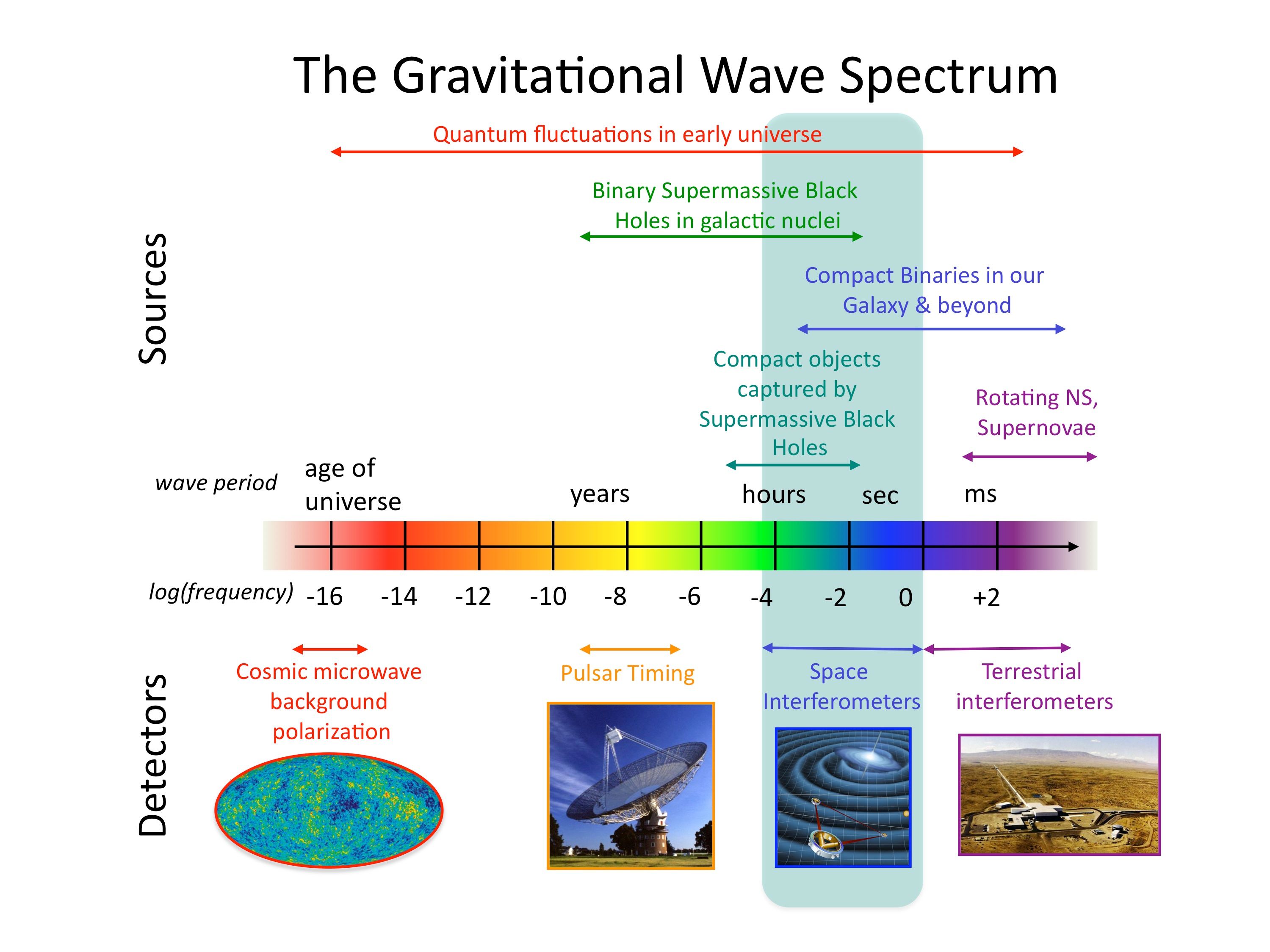
A highlight for next year: the first observing run of Advanced LIGO. Advanced LIGO is trying to make the first direct detection of gravitational waves. Gravitational waves are tiny stretches and squeezes in spacetime, to detect them you need to very carefully measure the distance between two points. This is where the 4 km arms come in: the Advanced LIGO detectors bounce lasers up and down their arms to measure the distance between the mirrors at the ends. The arms need to be as long as possible to make measuring the change in length as easy as possible. A typical change in length may be one part in 10²¹ (that is 1,000,000,000,000,000,000,000 or one sextillion… ). For comparison, that’s the same as measuring the distance between the Earth and the Sun to the diameter of a hydrogen atom or the distance from here to Alpha Centuri to the width of a human hair.

Aerial shot of LIGO Livingston, Louisiana. Two arms come out from the central building, one goes up the middle of the picture, the other goes off to the left out of shot. I think this gives a fair indication of the scale of the detectors. In addition to the instruments in Livingston, there is another LIGO in Hanford, Washington.

Making such an precise instrument is tricky. At least twice as tricky as remembering the names of all seven of the dwarfs. We shouldn’t be Bashful about saying how difficult it is. We need to keep the mirrors extremely still, any little wibbles from earth tremors, nearby traffic, or passing clouds need to be filtered out. Lots of clever Docs have been working on cunning means of keeping the mirrors still and then precisely measuring their position with the lasers. Some of that work was done here in Birmingham, in particular some of the mirror suspension systems. We’ll be rather Grumpy if those don’t work. However, things seem to be going rather well. Getting the mirrors working isn’t as simple as pushing a big red button, so it takes a while. On the 3 December, which is when we gave this talk at Astronomy in the City, the second detector achieved its first full lock: lock is when the mirrors are correctly held stably in position. This made me Happy. Also rather Sleepy, as it was a late night.

Team inspecting the optical systems at LIGO Livingston back at the start of 2014. (It’s a bit harder to detect the systems now, since they’re in a vacuum). You need to wear masks in case you are Sneezy, you’d feel rather Dopey if you ruined the mirrors by sneezing all over them. Credit: Michael Fyffe

5 (or more) planet-forming rings!

ALMA image of the planet-forming disc around HL Tau.

ALMA image of the young star HL Tau and its protoplanetary disc. The gaps in the disc indicate the formation of planets that sweep their orbits clear of dust and gas. Credit: ALMA, C. Brogan & B. Saxton

One of the most exciting discoveries of 2014 is this remarkable image of a planet-forming disc.There may be more than five planets, but it seemed like a shame not to fit this into our countdown here. The image is of the star HL Tauri. This is a young star, only a million years old (our Sun is about 4.6 billion years old). Remarkably, even at this young age, there seems to be indication of the formation of planets. The gaps are where planets have sucked up the dust, gas and loose change of the disc. This is the first time we’ve seen planet-formation in such detail, and matches predictions extremely well.

6 Frontier Fields

The six Frontier Fields are a group of six galaxy clusters that are being studied in unprecedented detail. They are being observing with three of NASA’s great observatories, the Hubble Space Telescope, the Spitzer Space Telescope (which observes in the infra-red) and the Chandra X-ray Observatory. These should allow us to measure all three components of the clusters (even the custard of the trifle). The clusters are all selected because the show strong gravitational lensing. This should give us excellent measurements of the mass of the clusters, and hence the distribution of dark matter.

Gravitational lensing by a galaxy cluster. The mass of the galaxy cluster bends spacetime. Light travelling through this curved spacetime is bent, just like passing through a lens. The amount of bending depends upon the mass, so we can weigh galaxy clusters by measuring the lensing. Credit: NASA, ESA & L. Calcada.

7 months until New Horizons reaches Pluto

New Horizons is a planetary mission to Pluto (and beyond). Launched in January 2006, New Horizons has been travelling through the Solar System ever since. In 2007 it made a fly-by of Jupiter, taking some amazing pictures. It is now just 7 months from reaching Pluto. This will give us the first ever detailed look at Pluto and its moons. You’ll need to wrap up warm if you wanted to head there yourself. I hope that New Horizons packed some mittens. New Horizons will tell us about Pluto and other icy (yes, that’s astronomers’ definition of ice again) items in the Kuiper belt.

Full trajectory of New Horizons, it’s come a long way! Credit: John Hopkins

New Horizons has been in hibernation for much of its flight. Who doesn’t like a good nap? New Horizons was woken up ahead of arriving at Pluto on 7 December. It got a special wake-up call from Russell Watson. I don’t think it has access to coffee though.

800 TB of data

This year’s Interstellar featured the most detailed simulations of the appearance of black holes. This involved a truly astounding amount of data. I’ve previously written about some of the science in Interstellar. I think it’s done a good at getting people interested in the topic of gravity. It’s scientific accuracy can be traced to the involvement of Kip Thorne, who has written a book on the film’s science (which might be a good Christmas present). Kip has done many things during his career, including being one of the pioneers of LIGO. After an exciting 2014 with the release of Interstellar, I’m sure he’s looking forward to 2015 and the first observations of Advanced LIGO too.

Light-bending around the black hole Gargantua in Interstellar. This shows the accretion disc about the black hole, the disc seen above and below the hole are actually the top and bottom of the disc behind the black hole. This extreme light-bending is a consequence of the extremely curved spacetime close to the black hole. This light-bending is exactly the same as the gravitational-lensing done by galaxy clusters, except much stronger!

999 Kepler exoplanets

When we gave the talk on 3 December, Kepler had discovered 998 exoplanets. It’s now 999, which I think means we get all the bonus points! Kepler is still doing good science, despite some technical difficulties. Kepler has been hugely successful. We now know that planets (as well as forming in quite short times) are common, that they are pretty much everywhere. Possibly even down the back of the sofa. Some of the work done here in Birmingham has been to estimate just how common planets are. On average, stars similar to the Sun have around 4 planets with periods shorter than 3 years (and radii bigger than 20% of Earth’s). That’s quite a few planets! But, if Christopher Nolan wants to direct another reasonably accurate sci-fi, we need to know how many of those are Earth-like. We don’t have enough data to work out details of atmospheres, but just looking at how many planets have a radius and period about the same as Earth’s, it seems that about 4% of these stars have Earth-like planets.

Kepler-186, a system which has a planet on the edge of the habitable zone.

Kepler-186, the first system discovered with an Earth-sized planet on the edge of the habitable zone (where liquid water could exist), was discovered in 2014.

10 lunar orbits

A Christmas highlight from 1968. On December 21, Apollo 8 launched. This was the first manned mission to ever leave Earth orbit. On Christmas Eve, it entered into orbit about the Moon. It’s three-man crew of Frank Borman, James Lovell and William Anders were the first people ever to orbit a body other than the Earth. To date, only 24 men have ever done so. Of course, even fewer have actually walked on the Moon, perhaps we should go back? Jim Lovell was also on the ill-fated Apollo 13 mission (you may have seen the film), making him the only person to orbit the Moon on two separate occasions and never land. Apollo 8 was successful, it orbited the Moon 10 times, giving us the first ever peek at the dark side of the moon (not the Pink Floyd album). This was also the first viewing of an Earthrise. Their Christmas Eve broadcast was most watched TV broadcast at the time. After orbiting, Apollo 8 returned home, splashing down December 27. I’m guessing they had a good New Year’s celebration!

Earthrise taken by the crew of Apollo 8, Christmas Eve 1968. Credit: NASA

11 (10 ¾) years for Rosetta

This year we landed on a comet. Rosetta has received fair amount of press. It is an amazing feat, Rosetta was in space for almost 11 years before making its comet rendezvous. It’ll be doing lots of science form orbit, such as determining that comets are unlikely to have delivered water to Earth. Most of the excitement surrounded the landing of Philae on the surface of the comet. That didn’t go quite as planned, but still taught us quite a bit. Rosetta has been heralded as one of the science breakthroughs of 2014. We’ll have to see what 2015 brings.

Colour image (yes, it’s grey) of 67P/Churyumov-Gerasimenko from Rosetta. Credit: ESA/Rosetta/MPS for OSIRIS Team MPS/UPD/LAM/IAA/SSO/INTA/UPM/DASP/IDA

12 (or more) galaxies in a cluster

To finish up, back to galaxy clusters. Galaxy clusters grow by merging. We throw two trifles together to get a bigger one. As you might imagine, if you throw two triffles together, you don’t get a nice, neat trifle. The layers do tend to mix. For galaxy clusters, you can get layers separating out: dark matter passes freely through everything, so it isn’t affected by a collision. The gas, however, does feel the shock and ends up a turbulent mess. It has been suggested that turbulence caused by mergers could trigger star formation: you squeeze the gas and some of it collapses down into stars. However, recent observational work at Birmingham can’t find any evidence for this. We’ll have to see if this riddle gets unravelled in 2015.

The merging bullet cluster. A composite of an optical image (showing galaxies), an X-ray image (in red, showing the hot gas), and a map of the total mass (in blue, from gravitational lensing). Dark matter, making up most of the mass, has past straight through the collision without interacting. Credit: NASA/CXC/CfA/STScI/ESO/U.Arizona/M. Markevitch/D. Clowe

Interstellar—science and fiction

November 8, 2014July 4, 2020 / CPLB / Leave a comment

Planet and accretion disc orbiting Gargantua, the black hole in Interstellar. Visual effects produced by the cunning people of Double Negative.

Interstellar is the latest film from Christopher Nolan. After completing his work with the Dark Knight, it seems he has moved onto even darker material: black holes. I have been looking forward to the film for some time, but not because of Nolan’s involvement (even though I have enjoyed his previous work). The film is based upon the ideas of Kip Thorne, an eminent theoretical physicist. Kip literally wrote the book on general relativity. He was a pioneer of gravitational-wave science, and earlier versions of the script included the detection of gravitational waves (I’m sad that this has been removed). Here, I’ll briefly discuss the film, before going on to look at it’s science (there are some minor spoilers).

My copies of Gravitation by Misner, Thorne & Wheeler, and General Theory of Relativity by Dirac. The difference in length might tell you something about the authors. MTW (as Gravitation is often called) is a useful textbook. It is so heavy that you can actually use it for experiments testing gravity.

Last week, my research group organised a meeting for our LIGO collaborators. We all got together in Birmingham to work on how we analyse gravitational-wave data. It was actually rather productive. We decided to celebrate the end of our meeting with a trip to see Interstellar. The consensus was that it was good. We were rather pleased by the amount of science in the film, undoubtedly due to Kip’s involvement (even if he doesn’t approve of everything)—we also liked how there was a robot called KIPP.

My favourite characters were, by far, the robots. They had more personality than any of the other characters: I was more concerned for their survival than for anyone else. (No-one was wearing red, but I thought it was quite obvious who was expendable). Michael Caine’s character is apparently based upon Kip—they do have similar beards.

The film is beautiful. Its visualisations have been much hyped (we’ll discuss these later). It shows an obvious debt to Kubrick’s 2001: A Space Odyssey. This is both for better and worse: mimicking the wonderful cinematography and the slow pacing. However, the conclusion lacks the mystery of 2001 or even the intelligence of Nolan’s earlier work Memento or Inception (both of which I would highly recommend).

I don’t want to say too much about the plot. I (unsurprisingly) approve of its pro-science perspective. There were some plot points that irked me. In particular, why on Earth (or off Earth) would a mission with the aim of continuing the human race only take one woman? Had no-one heard about putting all your eggs in one basket? Also, using Morse code to transmit complicated scientific data seems like a bad idea™. What if there were a typo? However, I did enjoy the action sequences and the few tense moments.

Why so scientific?

I expect that if you were after a proper film critique you’d be reading something else, so let’s discuss science. There is a lot of science in Interstellar, and I can’t go through it all, so I want to highlight a couple of pieces that I think are really cool.

Time is relative

An interesting story device is the idea that time is relative, and its passing depends upon where you are in gravitational field. This is entirely correct (and although time might flow at different apparent speeds, it never goes backwards). Imagine that you are tied to a length of extremely long and strong string, and lowered towards a black hole. (I wonder if that would make a good movie?) Let’s start off by considering a non-rotating black hole. The passage of time for you, relative to your friend with the other end of the string infinitely far away from the black hole, depends how close to the black hole you are. Times are related by

$\displaystyle \Delta T_\mathrm{infinity} = \left(1 - \frac{2 G M}{c^2 r}\right)^{-1/2} \Delta T_\mathrm{string}$ ,

where $M$ is the black hole’s mass, $G$ is Newton’s gravitational constant, $c$ is the speed of light, and $r$ measures how far you are from (the centre of) the black hole (more on this in a moment). If you were to flash a light every $\Delta T_\mathrm{string}$ , your friend at infinity would see them separated by time $\Delta T_\mathrm{infinity}$ ; it would be as if you were doing things in slow motion.

You might recognise $2GM/c^2$ as the location of the event horizon: the point of no return from a black hole. At the event horizon, we would be dividing by zero in the equation above, time would appear to run infinitely slowly for you. This is rather curious, time continues to run fine for you, but watching from infinity you would fade to a complete stand-still.

Actually, you would also fade from view too. The frequency of light gets shifted by gravity. Light is a wave, it’s frequency is set by how fast it completes one cycle. The period of the wave gets stretched using the formula above. As you get closer to a black hole, light from you becomes more red (then infra-red, radio, etc.), and also becomes dimmer (as less energy arrives at your friend at infinity in a given time). You appear to fade to to black as you approach the event horizon. This stretching of light to lower frequencies is known as red-shifting (as red light has the lowest frequencies of the visible spectrum). I didn’t see much sign of it in Interstellar (we’ll see the effect it should have had below), although it has appeared in an episode of Stargate: SG-1 as a plot device.

The event horizon is also the point where the force on the string would become infinite. Your friend at infinity would only be able to pull you back up if they ate an infinite amount of spinach, and sadly there is not enough balsamic dressing to go around.

A technicality that is often brushed over is what the distance $r$ actually measures. I said it tells you how how you are from the centre of the black hole, but it’s not as simple as dropping a tape measure in the see where the singularity is. In fact, we measure the distance differently. We instead measure the distance around the circumference of a circle, and divide this by $2\pi$ to calculate $r$ . The further away we are, the bigger the circle, and so the larger $r$ . If space were flat, this distance would be exactly the same as the distance to the middle, but when considering a black hole, we do not have flat space!

This time stretching due to gravity is a consequence of Einstein’s theory of general relativity. There is another similar effect in his theory of special relativity. If something travels past you with a speed $v$ , then time is slowed according to

$\displaystyle \Delta T_\mathrm{you} = \left(1 - \frac{v^2}{c^2}\right)^{-1/2} \Delta T_\mathrm{whizzing\:thing}$ .

If it were to travel closer and closer to the speed of light, the passage of time for it would slow to closer and closer to a standstill. This is just like crossing the event horizon.

Imagine that while you were sitting on the end of your string, a planet orbiting the black hole whizzed by. Someone of the planet flashes a torch every second (as they measure time), and when you see this, you flash your torch to your friend at infinity. The passage of time on the planet appears slowed to you because of the planet’s speed (using the special relativity formula above), and the passage of time for you appears slowed because of gravity to your friend at infinity. We can combine the two effects to work out the total difference in the apparent passage of time on the planet and at infinity. We need to know how fast the planet moves, but it’s not too difficult for a circular orbit, and after some algebra

$\displaystyle \Delta T_\mathrm{infinity} = \left(1 - \frac{3 G M}{c^2 r}\right)^{-1/2} \Delta T_\mathrm{planet}$ .

In Interstellar, there is a planet where each hour corresponds the seven years at a distance. That is a difference of about 61000. We can get this with our formula if $r \approx 3GM/c^2$ . Sadly, you can’t have a stable orbit inside $r = 6GM/c^2$ , so there wouldn’t be a planet there. However, the film does say that the black hole is spinning. This does change things (you can orbit closer in), so it should work out. I’ve not done the calculations, but I might give it a go in the future.

Black holes

Interstellar does an excellent job of representing a black hole. Black holes are difficult to visualise, but the film correctly depicts them as three-dimensional: they are not a two-dimensional hole.

As nothing escapes from a black hole (and they don’t have a surface), they are dark, a shadow on the sky. However, we can see their effects. The image at the top shows a disc about the black hole. Material falling into a black hole often has some angular momentum: it doesn’t fall straight in, but goes off to the side and swirls about, exactly as water whirls around the plug-hole before falling in. This material swirling around is known as an accretion disc. In the disc, things closer to the black hole are orbiting faster (just as planets closer to the Sun orbit faster than those further away). Hence different parts of the disc rub against each other. This slows the inner layers (making them lose angular momentum so that they move inwards), and also heats the disc. Try rubbing your hands together for a few seconds, they soon warm up. In an accretion disc about a black hole, things can become so hot (millions of degrees) that they emits X-rays. You wouldn’t want to get close because of this radiation! Looking for these X-rays is one way of spotting black holes.

The video below shows a simulation from NASA of an accretion disc about a black hole. It’s not quite as fancy as the Interstellar one, but it’s pretty cool. You can see the X-rays being red-shifted and blue-shifted (the opposite of red-shifted, when radiation gets squashed to higher frequencies) as a consequence of their orbital motion (the Doppler effect), but I’m not sure if it shows gravitational red-shifting.

Black holes bend spacetime, so light gets bent as it travels close to them. The video above shows this. You can see the light ring towards the centre, from light that has wrapped around the black hole. You can also see this in Interstellar. I especially like how the ring is offset to one side. This is exactly what you should expect for a rotating black hole: you can get closer in when you’re moving with the rotation of the black hole, getting swept around like a plastic duck around a whirlpool. You can also see how the disc appears bent as light from the back of the disc (which has to travel around the black hole) gets curved.

Light-bending and redshifting of an accretion disc around a black hole.

Light-bending around a black hole. This is figure 15 from James, von Tunzelmann, Franklin & Thorne (2015). The top image shows an accretion disc as seen in Interstellar, but without the lens flare. The middle image also includes (Doppler and gravitational) red-shifting that changes the colour of the light. To make the colour changes clear, the brightness has been artificially kept constant. The bottom image also includes the changes in brightness that would come with red-shifting. The left side of the disc is moving towards us, so it is brighter and blue-shifted, the right side is moving away so it is red-shifted. You can see (or rather can’t) how red-shifting causes things to fade from view. This is what the black hole and accretion disc would actually look like, but it was thought too confusing for the actual film.

It’s not only light from the disc that gets distorted, but light from stars (and galaxies) behind the black hole. This is known as gravitational lensing. This is one way of spotting black holes without accretion discs: you watch a field of stars and if a black hole passes in front of one, it’s gravitational lensing will magnify the star. Spotting that change tells you something has passed between you and the star, working our its mass and size can tell you if it’s a black hole.

Looking at the shadow of a black hole (the region from which there is no light, which is surrounded by the innermost light ring) can tell you about the structure of spacetime close to the black hole. This could give you an idea of its mass and spin, or maybe even test if it matches the predictions of general relativity. We are hoping to do this for the massive black hole at the centre of our Galaxy and the massive black hole of the galaxy Messier 87 (M87). This will be done using the Event Horizon Telescope, an exciting project to use several telescopes together to make extremely accurate images.

False-colour image of what the Event Horizon Telescope could see when look at Sagittarius A* (Dexter et al. 2010). Red-shifting makes some part of the the disc appear brighter and other parts dimmer.

Interstellar is science fiction, it contains many elements of fantasy. However, it does much better than most on getting the details of the physics correct. I hope that it will inspire many to investigate the fact behind the fiction (there’s now a paper out in Classical & Quantum Gravity about the visualisation of the black hole, it comes with some interesting videos). If you’ve not seen the film yet, it’s worth a watch. I wonder if they could put the gravitational waves back in for an extended DVD version?

Score out of 5 solar masses: enough for a neutron star, possibly not enough for a black hole.

Update: The Event Horizon Telescope Team did it! They have an image of M87’s black hole. It compares nicely to predictions. I’m impressed (definitely cake-worthy). Science has taken another bite out of science fiction.

The Event Horizon Telescope's image of M87*

The shadow of a black hole reconstructed from the radio observations of the Event Horizon Telescope. The black hole lies at the center of M87, and is about 6.5 billion solar masses. Credit: Event Horizon Team

The missing link for black holes

August 19, 2014September 2, 2020 / CPLB / Leave a comment

There has been some recent excitement about the claimed identification of a 400-solar-mass black hole. A team of scientists have recently published a letter in the journal Nature where they show how X-ray measurements of a source in the nearby galaxy M82 can be interpreted as originating from a black hole with mass of around 400 times the mass of the Sun—from now on I’ll use $M_\odot$ as shorthand for the mass of the Sun (one solar mass). This particular X-ray source is peculiarly bright and has long been suspected to potentially be a black hole with a mass around $100 M_\odot$ to $1000 M_\odot$ . If the result is confirmed, then it is the first definite detection of an intermediate-mass black hole, or IMBH for short, but why is this exciting?

Mass of black holes

In principle, a black hole can have any mass. To form a black hole you just need to squeeze mass down into a small enough space. For the something the mass of the Earth, you need to squeeze down to a radius of about 9 mm and for something about the mass of the Sun, you need to squeeze to a radius of about 3 km. Black holes are pretty small! Most of the time, things don’t collapse to form black holes because they materials they are made of are more than strong enough to counterbalance their own gravity.

These innocent-looking marshmallows could collapse down to form black holes if they were squeezed down to a size of about 10⁻²⁹ m. The only thing stopping this is the incredible strength of marshmallow when compared to gravity.

Stellar-mass black holes

Only very massive things, where gravitational forces are immense, collapse down to black holes. This happens when the most massive stars reach the end of their lifetimes. Stars are kept puffy because they are hot. They are made of plasma where all their constituent particles are happily whizzing around and bouncing into each other. This can continue to happen while the star is undergoing nuclear fusion which provides the energy to keep things hot. At some point this fuel runs out, and then the core of the star collapses. What happens next depends on the mass of the core. The least massive stars (like our own Sun) will collapse down to become white dwarfs. In white dwarfs, the force of gravity is balanced by electrons. Electrons are rather anti-social and dislike sharing the same space with each other (a concept known as the Pauli exclusion principle, which is a consequence of their exchange symmetry), hence they put up a bit of a fight when squeezed together. The electrons can balance the gravitational force for masses up to about $1.4 M_\odot$ , known as the Chandrasekhar mass. After that they get squeezed together with protons and we are left with a neutron star. Neutron stars are much like giant atomic nuclei. The force of gravity is now balanced by the neutrons who, like electrons, don’t like to share space, but are less easy to bully than the electrons. The maximum mass of a neutron star is not exactly known, but we think it’s somewhere between $2 M_\odot$ and $3 M_\odot$ . After this, nothing can resist gravity and you end up with a black hole of a few times the mass of the Sun.

Collapsing stars produce the imaginatively named stellar-mass black holes, as they are about the same mass as stars. Stars lose a lot of mass during their lifetime, so the mass of a newly born black hole is less than the original mass of the star that formed it. The maximum mass of stellar-mass black holes is determined by the maximum size of stars. We have good evidence for stellar-mass black holes, for example from looking at X-ray binaries, where we see a hot disc of material swirling around the black hole.

Massive black holes

We also have evidence for another class of black holes: massive black holes, MBHs to their friends, or, if trying to sound extra cool, supermassive black holes. These may be $10^5 M_\odot$ to $10^9 M_\odot$ . The strongest evidence comes from our own galaxy, where we can see stars in the centre of the galaxy orbiting something so small and heavy it can only be a black hole.

We think that there is an MBH at the centre of pretty much every galaxy, like there’s a hazelnut at the centre of a Ferrero Rocher (in this analogy, I guess the Nutella could be delicious dark matter). From the masses we’ve measured, the properties of these black holes is correlated with the properties of their surrounding galaxies: bigger galaxies have bigger MBHs. The most famous of these correlations is the M–sigma relation, between the mass of the black hole ( $M$ ) and the velocity dispersion, the range of orbital speeds, of stars surrounding it (the Greek letter sigma, $\sigma$ ). These correlations tell us that the evolution of the galaxy and it’s central black hole are linked somehow, this could be just because of their shared history or through some extra feedback too.

MBHs can grow by accreting matter (swallowing up clouds of gas or stars that stray too close) or by merging with other MBHs (we know galaxies merge). The rather embarrassing problem, however, is that we don’t know what the MBHs have grown from. There are really huge MBHs already present in the early Universe (they power quasars), so MBHs must be able to grow quickly. Did they grow from regular stellar-mass black holes or some form of super black hole that formed from a giant star that doesn’t exist today? Did lots of stellar-mass black holes collide to form a seed or did material just accrete quickly? Did the initial black holes come from somewhere else other than stars, perhaps they are leftovers from the Big Bang? We don’t have the data to tell where MBHs came from yet (gravitational waves could be useful for this).

Intermediate-mass black holes

However MBHs grew, it is generally agreed that we should be able to find some intermediate-mass black holes: black holes which haven’t grown enough to become IMBHs. These might be found in dwarf galaxies, or maybe in globular clusters (giant collections of stars that formed together), perhaps even in the centre of galaxies orbiting an MBH. Finding some IMBHs will hopefully tell us about how MBHs formed (and so, possibly about how galaxies formed too).

IMBHs have proved elusive. They are difficult to spot compared to their bigger brothers and sisters. Not finding any might mean we’d need to rethink our ideas of how MBHs formed, and try to find a way for them to either be born about a million times the mass of the Sun, or be guaranteed to grow that big. The finding of the first IMBH tells us that things are more like common sense would dictate: black holes can come in the expected range of masses (phew!). We now need to identify some more to learn about their properties as a population.

In conclusion, black holes can come in a range of masses. We know about the smaller stellar-mass ones and the bigger massive black holes. We suspect that the bigger ones grow from smaller ones, and we now have some evidence for the existence of the hypothesised intermediate-mass black holes. Whatever their size though, black holes are awesome, and they shouldn’t worry about their weight.

How does parameter estimation work?

Share this:

Parameter estimation

What we did

What we found

Notes

Share this:

Talks

Attendance

Share this:

Share this:

Share this:

Collaboration papers

Searching for gravitational waves from pulsars

Share this:

Share this:

A Newton under an apple tree

2 clear nights

3 components of a cluster

4 km long laser arms

5 (or more) planet-forming rings!

6 Frontier Fields

7 months until New Horizons reaches Pluto

800 TB of data

999 Kepler exoplanets

10 lunar orbits

11 (10 ¾) years for Rosetta

12 (or more) galaxies in a cluster

Share this:

Why so scientific?

Time is relative

Black holes

Share this:

Mass of black holes

Stellar-mass black holes

Massive black holes

Intermediate-mass black holes

Share this: