Advanced LIGO detects gravitational waves!

The first observing run (O1) of Advanced LIGO was scheduled to start 9 am GMT (10 am BST), 14 September 2015. Both gravitational-wave detectors were running fine, but there were few a extra things the calibration team wanted to do and not all the automated analysis had been set up, so it was decided to postpone the start of the run until 18 September. No-one told the Universe. At 9:50 am, 14 September there was an event. To those of us in the Collaboration, it is known as The Event.

Measured strain

The Event’s signal as measured by LIGO Hanford and LIGO Livingston. The shown signal has been filtered to make it more presentable. The Hanford signal is inverted because of the relative orientations of the two interferometers. You can clearly see that both observatories see that same signal, and even without fancy analysis, that there are definitely some wibbles there! Part of Fig. 1 from the Discovery Paper.

Detection

The detectors were taking data and the coherent WaveBurst (cWB) detection pipeline was set up analysing this. It finds triggers in near real time, and so about 3 minutes after the gravitational wave reached Earth, cWB found it. I remember seeing the first few emails… and ignoring them—I was busy trying to finalise details for our default parameter-estimation runs for the start of O1. However, the emails kept on coming. And coming. Something exciting was happening. The detector scientists at the sites swung in to action and made sure that the instruments would run undisturbed so we could get lots of data about their behaviour; meanwhile, the remaining data analysis codes were set running with ruthless efficiency.

The cWB algorithm doesn’t search for a particular type of signal, instead it looks for the same thing in both detectors—it’s what we call a burst search. Burst searches could find supernova explosions, black hole mergers, or something unexpected (so long as the signal is short). Looking at the data, we saw that the frequency increased with time, there was the characteristic chirp of a binary black hole merger! This meant that the searches that specifically look for the coalescence of binaries (black hole or neutron stars) should find it too, if the signal was from a binary black hole. It also meant that we could analyse the data to measure the parameters.

Time–frequency plot of The Event

A time–frequency plot that shows The Event’s signal power in the detectors. You can see the signal increase in frequency as time goes on: the characteristic chirp of a binary merger! The fact that you can spot the signal by eye shows how loud it is. Part of Fig. 1 from the Discovery Paper.

The signal was quite short, so it was quick for us to run parameter estimation on it—this makes a welcome change as runs on long, binary neutron-star signals can take months. We actually had the first runs done before all the detection pipelines had finished running. We kept the results secret: the detection people didn’t want to know the results before they looked at their own results (it reminded me of the episode of Whatever Happened to the Likely Lads where they try to avoid hearing the results of the football until they can watch the match). The results from each of the detection pipelines came in [bonus note]. There were the other burst searches: LALInferenceBurst found strong evidence for a signal, and BayesWave classified it clearly as a signal, not noise or a glitch; then the binary searches: both GstLAL and PyCBC found the signal (the same signal) at high significance. The parameter-estimation results were beautiful—we had seen the merger of two black holes!

At first, we couldn’t quite believe that we had actually made the detection. The signal seemed too perfect. Famously, LIGO conducts blind injections: fake signals are secretly put into the data to check that we do things properly. This happened during the run of initial LIGO (an event known as the Big Dog), and many people still remembered the disappointment. We weren’t set up for injections at the time (that was part of getting ready for O1), and the heads of the Collaboration said that there were no plans for blind injections, but people wanted to be sure. Only three or four people in the Collaboration can perform a blind injection; however, it’s a little publicised fact that you can tell if there was an injection. The data from the instruments is recorded at many stages, so there’s a channel which records the injected signal. During a blind-injection run, we’re not allowed to look at this, but this wasn’t a blind-injection run, so this was checked and rechecked. There was nothing. People considered other ways of injecting the signal that wouldn’t be recorded (perhaps splitting the signal up and putting small bits in lots of different systems), but no-one actually understands all the control systems well enough to get this to work. There were basically two ways you could fake the signal. The first is hack into the servers at both sites and CalTech simultaneously and modify the data before it got distributed. You would need to replace all the back-ups and make sure you didn’t leave any traces of tampering. You would also need to understand the control system well enough that all the auxiliary channels (the signal as recorded at over 30 different stages throughout the detectors’ systems) had the right data. The second is to place a device inside the interferometers that would inject the signal. As long as you had a detailed understanding of the instruments, this would be simple: you’d just need to break into both interferometers without being noticed. Since the interferometers are two of the most sensitive machines ever made, this is like that scene from Mission:Impossible, except on the actually impossible difficulty setting. You would need to break into the vacuum tube (by installing an airlock in the concrete tubes without disturbing the seismometers), not disturb the instrument while working on it, and not scatter any of the (invisible) infra-red laser light. You’d need to do this at both sites, and then break in again to remove the devices so they’re not found now that O1 is finished. The devices would also need to be perfectly synchronised. I would love to see a movie where they try to fake the signal, but I am convinced, absolutely, that the easiest way to inject the signal is to collide two black holes a billion years ago. (Also a good plot for a film?)

There is no doubt. We have detected gravitational waves. (I cannot articulate how happy I was to hit the button to update that page! [bonus note])

I still remember the exact moment this hit me. I was giving a public talk on black holes. It was a talk similar to ones I have given many times before. I start with introducing general relativity and the curving of spacetime, then I talk about the idea of a black hole. Next I move on to evidence for astrophysical black holes, and I showed the video zooming into the centre of the Milky Way, ending with the stars orbiting around Sagittarius A*, the massive black hole in the centre of our galaxy (shown below). I said that the motion of the stars was our best evidence for the existence of black holes, then I realised that this was no longer the case. Now, we have a whole new insight into the properties of black holes.

Gravitational-wave astronomy

Having caught a gravitational wave, what do you do with it? It turns out that there’s rather a lot of science you can do. The last few months have been exhausting. I think we’ve done a good job as a Collaboration of assembling all the results we wanted to go with the detection—especially since lots of things were being done for the first time! I’m sure we’ll update our analysis with better techniques and find new ways of using the data, but for now I hope everyone can enjoy what we have discovered so far.

I will write up a more technical post on the results, here we’ll run through some of the highlights. For more details of anything, check out the data release.

The source

The results of our parameter-estimation runs tell us about the nature of the source. We have a binary with objects of masses 36^{+5}_{-4} M_\odot and 29^{+4}_{-4} M_\odot, where M_\odot indicates the mass of our Sun (about 2 \times 10^{30} kilograms). If you’re curious what’s going with these numbers and the pluses and minuses, check out this bonus note.

Binary black hole masses

Estimated masses for the two black holes in the binary. m_1^\mathrm{source} is the mass of the heavier black hole and m_2^\mathrm{source} is the mass of the lighter black hole. The dotted lines mark the edge of our 90% probability intervals. The different coloured curves show different models: they agree which made me incredibly happy! Fig. 1 from the Parameter Estimation Paper.

We know that we’re dealing with compact objects (regular stars could never get close enough together to orbit fast enough to emit gravitational waves at the right frequency), and the only compact objects that can be as massive as these object are black holes. This means we’re discovered the first stellar-mass black hole binary! We’ve also never seen stellar-mass black holes (as opposed to the supermassive flavour that live in the centres of galaxies) this heavy, but don’t get too attached to that record.

Black holes have at most three properties. This makes them much simpler than a Starbucks Coffee (they also stay black regardless of how much milk you add). Black holes are described by their mass, their spin (how much they rotate), and their electric charge. We don’t expect black holes out in the Universe to have much electric charge because (i) its very hard to separate lots of positive and negative charge in the first place, and (ii) even if you succeed at (i), it’s difficult to keep positive and negative charge apart. This is kind of like separating small children and sticky things that are likely to stain. Since the electric charge can be ignored, we just need mass and spin. We’ve measured masses, can we measure spins?

Black hole spins are defined to be between 0 (no spin) and 1 (the maximum amount you can have). Our best estimates are that the bigger black hole has spin 0.3_{-0.3}^{+0.5}, and the small one has spin 0.5_{-0.4}^{+0.5} (these numbers have been rounded). These aren’t great measurements. For the smaller black hole, its spin is almost equally probable to take any allowed value; this isn’t quite the case, but we haven’t learnt much about its size. For the bigger black hole, we do slightly better, and it seems that the spin is on the smaller side. This is interesting, as measurements of spins for black holes in X-ray binaries tend to be on the higher side: perhaps there are different types of black holes?

We can’t measure the spins precisely for a few reasons. The signal is short, so we don’t see lots of wibbling while the binaries are orbiting each other (the tell-tale sign of spin). Results for the orientation of the binary also suggest that we’re looking at it either face on or face off, which makes any wobbles in the orbit that are there less visible. However, there is one particular combination of the spins, which we call the effective spin, that we can measure. The effective spin controls how the black holes spiral together. It has a value of 1 if both black holes have max spin values, and are rotating the same way as the binary is orbiting. It has a value of −1 if the black holes have max spin values and are both rotating exactly the opposite way to the binary’s orbit. We find that the effective spin is small, -0.06_{-0.18}^{+0.17}. This could mean that both black holes have small spins, or that they have larger spins that aren’t aligned with the orbit (or each other). We have learnt something about the spins, it’s just not too easy to tease that apart to give values for each of the black holes.

As the two black holes orbit each other, they (obviously, given what we’ve seen) emit gravitational waves. These carry away energy and angular momentum, so the orbit shrinks and the black holes inspiral together. Eventually they merge and settle down into a single bigger black hole. All this happens while we’re watching (we have great seats). A simulation of this happening is below. You can see that the frequency of the gravitational waves is twice that of the orbit, and the video freezes around the merger so you can see two become one.

What are the properties of the final black hole? The mass of the remnant black holes is 62^{+4}_{-4} M_\odot. It is the new record holder for the largest observed stellar-mass black hole!

If you do some quick sums, you’ll notice that the final black hole is lighter than the sum of the two initial black holes. This is because of that energy that was carried away by the gravitational waves. Over the entire evolution of the system, 3.0^{+0.5}_{-0.4} M_\odot c^2 \simeq 5.3_{-0.8}^{+0.9} \times 10^{47}~\mathrm{J} of energy was radiated away as gravitational waves (where c is the speed of light as in Einstein’s famous equation). This is a colossal amount of energy. You’d need to eat over eight billion times the mass of the Sun in butter to get the equivalent amount of calories. (Do not attempt the wafer-thin mint afterwards). The majority of that energy is radiated within the final second. For a brief moment, this one black hole merger outshines the whole visible Universe if you compare its gravitational-wave luminosity, to everything else’s visible-light luminosity!

We’ve measured mass, what about spin? The final black hole’s spin in 0.67^{+0.05}_{-0.07}, which is in the middling-to-high range. You’ll notice that we can deduce this to a much higher precisely than the spins of the two initial black holes. This is because it is largely fixed by the orbital angular momentum of the binary, and so its value is set by orbital dynamics and gravitational physics. I think its incredibly satisfying that we we can such a clean measurement of the spin.

We have measured both of the properties of the final black hole, and we have done this using spacetime itself. This is astounding!

Final black hole mass and spin

Estimated mass M_\mathrm{f}^\mathrm{source} and spin a_\mathrm{f}^\mathrm{source} for the final black hole. The dotted lines mark the edge of our 90% probability intervals. The different coloured curves show different models: they agree which still makes me incredibly happy! Fig. 3 from the Parameter Estimation Paper.

How big is the final black hole? My colleague Nathan Johnson-McDaniel has done some calculations and finds that the total distance around the equator of the black hole’s event horizon is about 1100~\mathrm{km} (about six times the length of the M25). Since the black hole is spinning, its event horizon is not a perfect sphere, but it bulges out around the equator. The circumference going over the black hole’s poles is about 1000~\mathrm{km} (about five and a half M25s, so maybe this would be the better route for your morning commute). The total area of the event horizon is about 37000~\mathrm{km}^2. If you flattened this out, it would cover an area about the size of Montana. Neil Cornish (of Montana State University) said that he’s not sure which we know more accurately: the area of the event horizon or the area of Montana!

OK, we’ve covered the properties of the black holes, perhaps it’s time for a celebratory biscuit and a sit down? But we’re not finished yet, where is the source?

We infer that the source is at a luminosity distance of 410^{+160}_{-180}~\mathrm{Mpc}, a megaparsec is a unit of length (regardless of what Han Solo thinks) equal to about 3 million light-years. The luminosity distance isn’t quite the same as the distance you would record using a tape measure because it takes into account the effects of the expansion of the Universe. But it’s pretty close. Using our 90% probability range, the merger would have happened sometime between 700 million years and 1.6 billion years ago. This coincides with the Proterozoic Eon on Earth, the time when the first oxygen-dependent animals appeared. Gasp!

With only the two LIGO detectors in operation, it is difficult to localise where on the sky source came from. To have a 90% chance of finding the source, you’d need to cover 600~\mathrm{deg^2} of the sky. For comparison, the full Moon is about 0.2~\mathrm{deg^2}. This is a large area to cover with a telescope, and we don’t expect there to be anything to see for a black hole merger, but that hasn’t stopped our intrepid partners from trying. For a lovely visualisation of where we think the source could be, marvel at the Gravoscope.

Astrophysics

The detection of this black hole merger tells us:

  • Black holes 30 times the mass of our Sun do form These must be the remains of really massive stars. Stars lose mass throughout their lifetime through stellar winds. How much they lose depends on what they are made from. Astronomers have a simple periodic table: hydrogen, helium and metals. (Everything that is not hydrogen or helium is a metal regardless of what it actually is). More metals means more mass loss, so to end up with our black holes, we expect that they must have started out as stars with less than half the fraction of metals found in our Sun. This may mean the parent stars were some of the first stars to be born in the Universe.
  • Binary black holes exist There are two ways to make a black hole binary. You can start with two stars in a binary (stars love company, so most have at least one companion), and have them live their entire lives together, leaving behind the two black holes. Alternatively, you could have somewhere where there are lots of stars and black holes, like a globular cluster, and the two black holes could wander close enough together to form the binary. People have suggested that either (or both) could happen. You might be able to tell the two apart using spin measurements. The spins of the black holes are more likely to be aligned (with each other and the way that the binary orbits) if they came from stars formed in a binary. The spins would be randomly orientated if two black holes came together to form a binary by chance. We can’t tell the two apart now, but perhaps when we have more observations!
  • Binary black holes merge Since we’ve seen a signal from two black holes inspiralling together and merging, we know that this happens. We can also estimate how often this happens, given how many signals we’ve seen in our observations. Somewhere in the observable Universe, a similar binary could be merging about every 15 minutes. For LIGO, this should mean that we’ll be seeing more. As the detectors’ sensitivity improves (especially at lower frequencies), we’ll be able to detect more and more systems [bonus note]. We’re still uncertain in our predictions of exactly how many we’ll see. We’ll understand things better after observing for longer: were we just lucky, or were we unlucky not to have seen more? Given these early results, we estimate that the end of the third observing run (O3), we could have over 30. It looks like I will be kept busy over the next few years…

Gravitational physics

Black holes are the parts of the Universe with the strongest possible gravity. They are the ideal place to test Einstein’s theory of general relativity. The gravitational waves from a black hole merger let us probe right down to the event horizon, using ripples in spacetime itself. This makes gravitational waves a perfect way of testing our understanding of gravity.

We have run some tests on the signal to see how well it matches our expectations. We find no reason to doubt that Einstein was right.

The first check is that if we try to reconstruct the signal, without putting in information about what gravitational waves from a binary merger look like, we find something that agrees wonderfully with our predictions. We can reverse engineer what the gravitational waves from a black hole merger look like from the data!

Estimated waveforms from different models

Recovered gravitational waveforms from our analysis of The Event. The dark band shows our estimate for the waveform without assuming a particular source (it is build from wavelets, which sound adorable to me). The light bands show results if we assume it is a binary black hole (BBH) as predicted by general relativity. They match really well! Fig. 6 from the Parameter Estimation Paper.

As a consistency test, we checked what would happen if you split the signal in two, and analysed each half independently with our parameter-estimation codes. If there’s something weird, we would expect to get different results. We cut the data into a high frequency piece and a low frequency piece at roughly where we think the merger starts. The lower frequency (mostly) inspiral part is more similar to the physics we’ve tested before, while the higher frequency (mostly) merger and ringdown is new and hence more uncertain. Looking at estimates for the mass and spin of the final black hole, we find that the two pieces are consistent as expected.

In general relativity, gravitational waves travel at the speed of light. (The speed of light is misnamed, it’s really a property of spacetime, rather than of light). If gravitons, the theoretical particle that carries the gravitational force, have a mass, then gravitational waves can’t travel at the speed of light, but would travel slightly slower. Because our signals match general relativity so well, we can put a limit on the maximum allowed mass. The mass of the graviton is less than 1.2 \times 10^{-22}~\mathrm{eV\,c^{-2}} (in units that the particle physicists like). This is tiny! It is about as many times lighter than an electron as an electron is lighter than a teaspoon of water (well, 4~\mathrm{g}, which is just under a full teaspoon), or as many times lighter than the almost teaspoon of water is than three Earths.

Limits on the Compton wavelength of the graviton

Bounds on the Compton wavelength \lambda_g of the graviton from The Event (GW150914). The Compton wavelength is a length defined by the mass of a particle: smaller masses mean large wavelengths. We place much better limits than existing tests from the Solar System or the double pulsar. There are some cosmological tests which are stronger still (but they make assumptions about dark matter). Fig. 8 from the Testing General Relativity Paper.

Overall things look good for general relativity, it has passed a tough new test. However, it will be extremely exciting to get more observations. Then we can combine all our results to get the best insights into gravity ever. Perhaps we’ll find a hint of something new, or perhaps we’ll discover that general relativity is perfect? We’ll have to wait and see.

Conclusion

100 years after Einstein predicted gravitational waves and Schwarzschild found the equations describing a black hole, LIGO has detected gravitational waves from two black holes orbiting each other. This is the culmination of over forty years of effort. The black holes inspiral together and merge to form a bigger black hole. This is the signal I would have wished for. From the signal we can infer the properties of the source (some better than others), which makes me exceedingly happy. We’re starting to learn about the properties of black holes, and to test Einstein’s theory. As we continue to look for gravitational waves (with Advanced Virgo hopefully joining next year), we’ll learn more and perhaps make other detections too. The era of gravitational-wave astronomy has begun!

After all that, I am in need of a good nap! (I was too excited to sleep last night, it was like a cross between Christmas Eve and the night before final exams). For more on the story from scientists inside the LIGO–Virgo Collaboration, check out posts by:

  • Matt Pitkin (the tireless reviewer of our parameter-estimation work)
  • Brynley Pearlstone (who’s just arrived at the LIGO Hanford site)
  • Amber Stuver (who  blogged through LIGO’s initial runs too)
  • Rebecca Douglas (a good person to ask about what build a detector out of)
  • Daniel Williams (someone fresh to the Collaboration)
  • Sean Leavey (a PhD student working on on interferometry)
  • Andrew Williamson (who likes to look for gravitational waves that coincide with gamma-ray bursts)
  • Shane Larson (another fan of space-based gravitational-wave detectors)
  • Roy Williams (who helps to make all the wonderful open data releases for LIGO)
  • Chris North (creator of the Gravoscope amongst other things)

There’s also this video from my the heads of my group in Birmingham on their reactions to the discovery (the credits at the end show how large an effort the detection is).

Discovery paper: Observation of Gravitational Waves from a Binary Black Hole Merger
Date release:
LIGO Open Science Center

Bonus notes

Search pipelines

At the Large Hadron Collider, there are separate experiments that independently analyse data, and this is an excellent cross-check of any big discoveries (like the Higgs). We’re not in a position to do this for gravitational waves. However, the different search pipelines are mostly independent of each other. They use different criteria to rank potential candidates, and the burst and binary searches even look for different types of signals. Therefore, the different searches act as a check of each other. The teams can get competitive at times, so they do check each other’s results thoroughly.

The announcement

Updating Have we detected gravitational waves yet? was doubly exciting as I had to successfully connect to the University’s wi-fi. I managed this with about a minute to spare. Then I hovered with my finger on the button until David Reitze said “We. Have detected. Gravitational waves!” The exact moment is captured in the video below, I’m just off to the left.

Univeristy of Birmingham detection announcement

The moment of the announcement of the first observation of gravitational waves at the University of Birmingham. Credit: Kat Grover

Parameters and uncertainty

We don’t get a single definite number from our analysis, we have some uncertainty too. Therefore, our results are usually written  as the median value (which means we think that the true value is equally probable to be above or below this number), plus the range needed to safely enclose 90% of the probability (so there’s a 10% chance the true value is outside this range. For the mass of the bigger black hole, the median estimate is 36 M_\odot, we think there’s a 5% chance that the mass is below 32 M_\odot =(36 - 4) M_\odot, and a 5% chance it’s above 41 M_\odot =(36 + 5) M_\odot, so we write our result as 36^{+5}_{-4} M_\odot.

Sensitivity and ranges

Gravitational-wave detectors measure the amplitude of the wave (the amount of stretch and squash). The measured amplitude is smaller for sources that are further away: if you double the luminosity distance of a source, you halve its amplitude. Therefore, if you improve your detectors’ sensitivity by a factor of two, you can see things twice as far away. This means that we observe a volume of space (2 × 2 × 2) = 8 times as big. (This isn’t exactly the case because of pesky factors from the expansion of the Universe, but is approximately right). Even a small improvement in sensitivity can have a considerable impact on the number of signals detected!

Advertisement

Neutrino oscillations and Nobel Prizes

This year’s Nobel Prize in Physics was awarded to Takaaki Kajita and Arthur McDonald for the discovery of neutrino oscillations. This is some really awesome physics which required some careful experimentation and some interesting new theory; it is also one of the things that got me interested in astrophysics.

Neutrinos

Neutrinos are an elusive type of subatomic particle. They are sometimes represented by the Greek letter nu \nu, and their antiparticle equivalents (antineutrinos) are denoted by \bar{\nu}. We’ll not worry about the difference between the two. Neutrinos are rather shy. They are quite happy doing their own thing, and don’t interact much with other particles. They don’t have an electric charge (they are neutral), so they don’t play with the electromagnetic force (and photons), they also don’t do anything with the strong force (and gluons). They only get involved with the weak force (W and Z bosons). As you might expect from the name, the weak force doesn’t do much (it only operates over short distances), so spotting a neutrino is a rare occurrence.
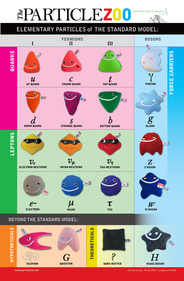
Particle Zoo

The charming bestiary of subatomic particles made by Particle Zoo.

There is a large family of subatomic particles. The electron is one of the most familiar, being a component of atoms (and hence you, me, cake and even marshmallows). The electron has two cousins: the muon (not to be confused with the moo-on) and the tau particle. All three have similar characteristics, with the only real difference being their mass. Electrons are the lightest, muons are about 207 times heavier, and tau are about 17 times heavier still (3477 times the mass of the electron). Each member of the electron family has a neutrino counterpart: there’s the electron-neutrino \nu_e, the muon-neutrino \nu_\mu (\mu is the Greek letter mu) and the tau-neutrino \nu_\tau (\tau is the Greek letter tau).

Neutrinos are created and destroyed in in certain types of nuclear reactions. Each flavour of neutrino is only involved in reactions that involve their partner from the electron family. If an electron-neutrino is destroyed in a reaction, an electron is created; if a muon is destroyed, a muon-neutrino is created, and so on.

Solar neutrinos

Every second, around sixty billion neutrinos pass through every square centimetre on the Earth. Since neutrinos so rarely interact, you would never notice them. The source of these neutrinos is the Sun. The Sun is powered by nuclear fusion. Hydrogen is squeezed into helium through a series of nuclear reactions. As well as producing the energy that keeps the Sun going, these create lots of neutrinos.

The pp chain

The nuclear reactions that power the Sun. Protons (p), which are the nuclei of hydrogen, are converted to Helium nuclei after a sequence of steps. Electron neutrinos \nu_e are produced along the way. This diagram is adapted from Giunti & Kim. The traditional names of the produced neutrinos are given in bold and the branch names are given in parentheses and percentages indicate branching fractions.

The neutrinos produced in the Sun are all electron-neutrinos. Once made in the core of the Sun, they are free to travel the 700,000 km to the surface of the Sun and then out into space (including to us on Earth). Detecting these neutrinos therefore lets you see into the very heart of the Sun!

Solar neutrinos were first detected by the Homestake experiment. This looked for the end results of nuclear reactions caused when an electron-neutrino is absorbed. Basically, it was a giant tub of dry-cleaning fluid. This contains chlorine, which turns to argon when a neutrino is absorbed. The experiment had to count how many atoms of argon where produced. In 1968, the detection was announced. However, we could only say that there were neutrinos around, not that they were coming from the Sun…

To pin down where the neutrinos were coming from required a new experiment. Deep in the Kamioka Mine, Kamiokande looked for interactions between neutrinos and electrons. Very rarely a neutrino will bump into an electron. This can give the electron a big kick (since the neutrino has a lot of momentum). Kamiokande had a large tank of water (and so lots of electrons to hit). If one got a big enough kick, it could travel faster than the speed of light in water (about 2/3 of the speed of light in vacuum). It then emits a flash of light called Cherenkov radiation, which is the equivalent of the sonic boom created when a plane travels faster than the speed of sound. Looking where the light comes from tells you where the electron was coming from and so where the neutrino came from. Tracing things back, it was confirmed that the neutrinos were coming from the Sun!

This discovery confirmed that the Sun was powered by fusion. I find it remarkable that it was only in the late 1980s that we had hard evidence for what was powering the Sun (that’s within my own lifetime). This was a big achievement, and Raymond Davies Jr., the leader of the Homestake experiment, and Masatoshi Koshiba, the leader of the Kamiokande experiment, were awarded the 2002 Nobel Prize in Physics for pioneering neutrino astrophysics. This also led to one of my all-time favourite pictures: the Sun at night.

The Sun at night!

The Sun at night. Solar neutrinos as detected by Super-Kamioknade looking through the Earth. I think this is the astronomical equivalent of checking if the fridge light does go off when you close the door. Credit: Marcus Chown & Super-Kamiokande.

The mystery of the missing neutrinos

Detecting solar neutrinos was a big success, but there was a problem. There were only a fraction of the predicted number. This became known as the solar neutrino problem. There were two possibilities, either solar physicists had got their models wrong, or particle physicists were missing a part of the Standard Model.

The solar models were recalculated and tweaked, with much work done by John Bahcall and collaborators. More sophisticated calculations were performed, even folding in new data from helioseismology, the study of waves in the Sun, but the difference could not be resolved.

However, there was an idea in particle physics by Bruno Pontecorvo and Vladimir Gribov: that neutrinos could change flavour, a phenomena known as neutrino oscillations. This was actually first suggested before the first Homestake results were announced, perhaps it deserved further attention?

The first evidence in favour of neutrino oscillations comes from Super-Kamiokande, the successor to the original Kamiokande. This evidence came from looking at neutrinos produced by cosmic rays. Cosmic rays are highly energetic particles that come from space. As they slam into the atmosphere, and collide with molecules in the air, they produce a shower of particles. These include muons and muon-neutrinos. Super-Kamiokande could detect muon-neutrinos from cosmic rays. Cosmic rays come from all directions, so Super-Kamiokande should see muon-neutrinos from all directions too. Just like we can see the solar neutrinos through the Earth, we should see muon-neutrinos both from above and below. However, more were detected from above than below.

Something must happen to muon-neutrinos during their journey through the Earth. Super-Kamiokande could detect them as electron-neutrinos or muon-neutrinos, but is not sensitive to tau-neutrinos. This is evidence that muon-neutrinos were changing flavour to tau-neutrinos.

Sudbury Neutrino Observatory

The Sudbury Neutrino Observatory detector, a 12-metre sphere containing 1000 tonnes of heavy water which is two kilometres underground. Credit: SNOLAB.

The solar neutrino problem was finally solved in 2001 through measurements of the Sudbury Neutrino Observatory (SNO). SNO is another Cherenkov detector like (Super-)Kamiokande, but it used heavy water instead of regular water. (High-purity heavy water is extremely expensive, it would have cost hundreds of millions of dollars for SNO to buy the 1000 tonnes it used, so it managed to secure it on loan from Atomic Energy of Canada Limited). Using heavy water meant that SNO was sensitive to all flavours of neutrinos. Like previous experiments, SNO found that there were not as many electron-neutrinos from the Sun as expected. However, there were also muon-neutrinos and tau-neutrinos, and when these were added, the total worked out!

The solar astrophysicists had been right all along, what was missing was that neutrinos oscillate between flavours. Studying the Sun had led to a discovery about some of the smallest particles in Nature.

Neutrino oscillations

Experiments have shown that neutrino oscillations occur, but how does this work? We need to delve into quantum mechanics.

The theory of neutrino oscillations say that each of the neutrino flavours corresponds to a different combination of neutrino mass states. This is weird, it means that if you were to somehow weight an electron-, muon- or tau-neutrino, you would get one of three values, but which one is random (although on average, each flavour would have a particular mass). By rearranging the mass states into a different combination you can get a different neutrino flavour. While neutrinos are created as a particular flavour, when they travel, the mass states rearrange relative to each other, so when they arrive at their destination, they could have changed flavour (or even changed flavour and then changed back again).

To get a more detailed idea of what’s going on, we’ll imagine the simpler case of there being only two neutrino flavours (and two neutrino mass states). We can picture a neutrino as a clock face with an hour hand and a minute hand. These represent the two mass states. Which neutrino flavour we have depends upon their relative positions. If they point in the same direction, we have one flavour (let’s say mint) and if they point in opposite directions, we have the other (orange). We’ll create a mint neutrino at 12 noon and watch it evolve. The hands more at different speeds, so at ~12:30 pm, they are pointing opposite ways, and our neutrino has oscillated into an orange neutrino. At ~1:05 pm, the hands are aligned again, and we’re back to mint. Which neutrino you have depends when you look. At 3:30 am, you’ll have a roughly even chance of finding either flavour and at 6:01 pm, you’ll be almost certain to have orange neutrino, but there’s still a tiny chance of finding an mint one. As time goes on, the neutrino oscillates back and forth.

With three neutrinos flavours, things are more complicated, but the idea is similar. You can imagine throwing in a second hand and making different flavours based upon the relative positions of all three hands.

We can now explain why Super-Kamiokande saw different numbers of muon-neutrinos from different sides of the Earth. Those coming from above only travel a short distance, there’s little time between when they were created and when they are detected, so there’s not much chance they’ll change flavour. Those coming through the Earth have had enough time to switch flavour.

A similar thing happens as neutrinos travel from the core of the Sun out to the surface. (There’s some interesting extra physics that happens here too. A side effect of there being so much matter at the centre of the Sun, the combination of mass states that makes up the different flavours is different than at the outside. This means that even without the hands on the clock going round, we can get a change in flavour).

Neutrino oscillations happen because neutrino mass states are not the same as the flavour states. This requires that neutrinos have mass. In the Standard Model, neutrinos are massless, so the Standard Model had to be extended.

2015 Physics Nobel laureates

2015 Physics Nobel laureates, Takaaki Kajita and Arthur B. McDonald. Credit: Nobel Foundation.

Happy ending

For confirming that neutrinos have mass, Takaaki Kajita of Super-Kamiokande and Arthur McDonald of SNO won this year’s Nobel Prize. It is amazing how much physics has been discovered from trying to answer as simple a question as how does the Sun shine?

Even though neutrinos are shy, they are really interesting characters when you get to know them.

Now that the mystery of the missing neutrinos is solved, what is next? Takaaki Kajita is now involved in another project in the Kamioka Mine, the construction of KAGRA, a gravitational-wave detector.

KAGRA control room

The control room of KAGRA, the gravitational-wave detector in the Hida Mountains, Japan. I visited June 2015. Could a third Nobel come out of the Kamioka Mine?

LIGO Magazine: Issue 7

It is an exciting time time in LIGO. The start of the first observing run (O1) is imminent. I think they just need to sort out a button that is big enough and red enough (or maybe gather a little more calibration data… ), and then it’s all systems go. Making the first direct detection of gravitational waves with LIGO would be an enormous accomplishment, but that’s not all we can hope to achieve: what I’m really interested in is what we can learn from these gravitational waves.

The LIGO Magazine gives a glimpse inside the workings of the LIGO Scientific Collaboration, covering everything from the science of the detector to what collaboration members like to get up to in their spare time. The most recent issue was themed around how gravitational-wave science links in with the rest of astronomy. I enjoyed it, as I’ve been recently working on how to help astronomers look for electromagnetic counterparts to gravitational-wave signals. It also features a great interview with Joseph Taylor Jr., one of the discoverers of the famous Hulse–Taylor binary pulsar. The back cover features an article I wrote about parameter estimation: an expanded version is below.

How does parameter estimation work?

Detecting gravitational waves is one of the great challenges in experimental physics. A detection would be hugely exciting, but it is not the end of the story. Having observed a signal, we need to work out where it came from. This is a job for parameter estimation!

How we analyse the data depends upon the type of signal and what information we want to extract. I’ll use the example of a compact binary coalescence, that is the inspiral (and merger) of two compact objects—neutron stars or black holes (not marshmallows). Parameters that we are interested in measuring are things like the mass and spin of the binary’s components, its orientation, and its position.

For a particular set of parameters, we can calculate what the waveform should look like. This is actually rather tricky; including all the relevant physics, like precession of the binary, can make for some complicated and expensive-to-calculate waveforms. The first part of the video below shows a simulation of the coalescence of a black-hole binary, you can see the gravitational waveform (with characteristic chirp) at the bottom.

We can compare our calculated waveform with what we measured to work out how well they fit together. If we take away the wave from what we measured with the interferometer, we should be left with just noise. We understand how our detectors work, so we can model how the noise should behave; this allows us to work out how likely it would be to get the precise noise we need to make everything match up.

To work out the probability that the system has a given parameter, we take the likelihood for our left-over noise and fold in what we already knew about the values of the parameters—for example, that any location on the sky is equally possible, that neutron-star masses are around 1.4 solar masses, or that the total mass must be larger than that of a marshmallow. For those who like details, this is done using Bayes’ theorem.

We now want to map out this probability distribution, to find the peaks of the distribution corresponding to the most probable parameter values and also chart how broad these peaks are (to indicate our uncertainty). Since we can have many parameters, the space is too big to cover with a grid: we can’t just systematically chart parameter space. Instead, we randomly sample the space and construct a map of its valleys, ridges and peaks. Doing this efficiently requires cunning tricks for picking how to jump between spots: exploring the landscape can take some time, we may need to calculate millions of different waveforms!

Having computed the probability distribution for our parameters, we can now tell an astronomer how much of the sky they need to observe to have a 90% chance of looking at the source, give the best estimate for the mass (plus uncertainty), or even figure something out about what neutron stars are made of (probably not marshmallow). This is the beginning of gravitational-wave astronomy!

Monty and Carla map parameter space

Monty, Carla and the other samplers explore the probability landscape. Nutsinee Kijbunchoo drew the version for the LIGO Magazine.

Puzzle procrastination: perplexing probabilities part II

A while ago I set some probability puzzles. If you’ve not yet pondered them, give them a whirl now. It’s OK, I’ll wait… All done? Final answer?

1 Girls, boys and doughnuts

We know that Laura has two children. There are four possibilities: two girls (\mathrm{GG}
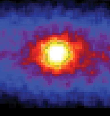
), a boy and a girl (\mathrm{BG}), a girl and a boy (\mathrm{GB}) and two boys (\mathrm{BB}). The probability of having a boy is almost identical to having a girl, so let’s keep things simple and assume that all four options have equal probability.

In this case, (i) the probability of having two girls is P(\mathrm{GG}) = 1/4; (ii) the probability of having a boy and a girl is P(\mathrm{B,\,G}) = P(\mathrm{BG}) + P(\mathrm{GB}) = 1/2, and (iii) the probability of having two boys is P(\mathrm{BB}) = 1/4.

After meeting Laura’s daughter Lucy, we know she doesn’t have two boys. What are the probabilities now? There are three options left (\mathrm{GG}, \mathrm{GB} and \mathrm{BG}), but they are not all equally likely. We’ve discussed a similar problem before (it involved water balloons). You can work out the probabilities using Bayes’ Theorem, but let’s see if we can get away without using any maths more complicated than addition. Lucy could either be the elder or the younger child, each is equally likely. There must be four possible outcomes: Lucy and then another girl (\mathrm{LG}), another girl and then Lucy (\mathrm{GL}), Lucy and then a boy (\mathrm{LB}) or a boy and then Lucy (\mathrm{BL}). Since the sex of children are not linked (if we ignore the possibility of identical twins), each of these are equally probable. Therefore, (i) P(\mathrm{GG}) = P(\mathrm{LG}) + P(\mathrm{GL}) = 1/2; (ii) P(\mathrm{B,\,G}) = P(\mathrm{LB}) + P(\mathrm{BL}) = 1/2, and (iii) P(\mathrm{BB}) = 0. We have ruled out one possibility, and changed the probability having two girls.

If we learn that Lucy is the eldest, then we are left with two options, \mathrm{LG} and \mathrm{LB}. This means (i) P(\mathrm{GG}) = P(\mathrm{LG}) = 1/2; (ii) P(\mathrm{B,\,G}) = P(\mathrm{LB}) = 1/2, and (iii) P(\mathrm{BB}) = 0. The probabilities haven’t changed! This is because the order of birth doesn’t influence the probability of being a boy or a girl.

Hopefully that all makes sense so far. Now let’s move on to Laura’s secret society for people who have two children of which at least one is a girl. There are three possibilities for the children: \mathrm{GG}, \mathrm{BG} or \mathrm{GB}. This time, all three are equally likely as we are just selecting them equally from the total population. Families with two children are equally likely to have each of the four combinations, but those with \mathrm{BB} are turned away at the door, leaving an equal mix of the other three. Hence,  (i)  P(\mathrm{GG}) = 1/3; (ii) P(\mathrm{B,\,G}) = P(\mathrm{BG}) + P(\mathrm{GB}) = 2/3, and (iii) P(\mathrm{BB}) = 0.

The probabilities are different in this final case than for Laura’s family! This is because of the difference in the way we picked are sample. With Laura, we knew she had two children, the probability that she would have a daughter with her depends upon how many daughters she has. It’s more likely that she’d have a daughter with her if she has two, than one (or zero). If we’re picking families with at least one girl at random, things are different. This has confused enough people to be known as the boy or girl paradox. However, if you’re careful in writing things down, it’s not too tricky to work things out.

2 Do or do-nut

You’re eating doughnuts, and trying to avoid the one flavour you don’t like. After eating six of twenty-four you’ve not encountered it. The other guests have eaten twelve, but that doesn’t tell you if they’ve eaten it. All you know is that it’s not in the six you’ve eaten, hence it must be one of the other eighteen. The probability that one of the twelve that the others have eaten is the nemesis doughnut is P(\mathrm{eaten}) = 12/18 = 2/3. Hence, the probability it is left is P(\mathrm{left}) = 1 - P(\mathrm{eaten}) = 1/3. Since there are six doughnuts left, the probability you’ll pick the nemesis doughnut next is P(\mathrm{next}) = P(\mathrm{left}) \times 1/6 = 1/18. Equally, you could have figured that out by realising that it’s equally probable that the nemesis doughnut is any of the eighteen that you’ve not eaten.

When twelve have been eaten, Lucy takes one doughnut to feed the birds. You all continue eating until there are four left. At this point, no-one has eaten that one doughnut. There are two possible options: either it’s still lurking or it’s been fed to the birds. Because we didn’t get to use it in the first part, I’ll use Bayes’ Theorem to work out the probabilities for both options.

The probability that Lucy luckily picked that one doughnut to feed to the birds is P(\mathrm{lucky}) = 1/12, the probability that she unluckily picked a different flavour is P(\mathrm{unlucky}) = 1 - P(\mathrm{lucky}) = 11/12. If we were lucky, the probability that we managed to get down to there being four left is P(\mathrm{four}|\mathrm{lucky}) = 1, we were guaranteed not to eat it! If we were unlucky, that the bad one is amongst the remaining eleven, the probability of getting down to four is P(\mathrm{four}|\mathrm{unlucky}) = 4/11. The total probability of getting down to four is

P(\mathrm{four}) = P(\mathrm{four}|\mathrm{lucky})P(\mathrm{lucky}) + P(\mathrm{four}|\mathrm{unlucky})P(\mathrm{unlucky}).

Substituting in gives

\displaystyle P(\mathrm{four}) = 1 \times \frac{1}{12} + \frac{4}{11} \times \frac{11}{12} = \frac{5}{12}.

The probability that the doughnut is not left is when there are four left is

\displaystyle P(\mathrm{lucky}|\mathrm{four}) = \frac{P(\mathrm{four}|\mathrm{lucky})P(\mathrm{lucky})}{P(\mathrm{four})},

putting in the numbers gives

\displaystyle P(\mathrm{lucky}|\mathrm{four}) = 1 \times \frac{1}{12} \times \frac{12}{5} = \frac{1}{5}.

The probability that it’s left must be

\displaystyle P(\mathrm{unlucky}|\mathrm{four}) = \frac{4}{5}.

We could’ve worked this out more quickly by realised that there are five doughnuts that could potential be the one: the four left and the one fed to the birds. Each one is equally probable, so that gives P(\mathrm{lucky}|\mathrm{four}) = 1/5 and P(\mathrm{unlucky}|\mathrm{four}) = 4/5.

If you take one doughnut each, one after another, does it matter when you pick? You have an equal probability of each being the one. The probability that it’s the first is

\displaystyle P(\mathrm{first}) = \frac{1}{4} \times P(\mathrm{unlucky}|\mathrm{four}) = \frac{1}{5};

the probability that it’s the second is

\displaystyle P(\mathrm{second}) = \frac{1}{3} \times \frac{3}{4} \times P(\mathrm{unlucky}|\mathrm{four}) = \frac{1}{5};

the probability that it’s the third is

\displaystyle P(\mathrm{third}) = \frac{1}{2} \times \frac{2}{3} \times \frac{3}{4} \times P(\mathrm{unlucky}|\mathrm{four}) = \frac{1}{5},

and the probability that it’s the fourth (last) is

\displaystyle P(\mathrm{third}) = 1 \times \frac{1}{2} \times \frac{2}{3} \times \frac{3}{4} \times P(\mathrm{unlucky}|\mathrm{four}) = \frac{1}{5}.

That doesn’t necessarily mean it doesn’t matter when you pick though! That really depends how you feel when taking an uncertain bite, how much you value the knowledge that you can safely eat your doughnut, and how you’d feel about skipping your doughnut rather than eating one you hate.

Gravitational-wave sensitivity curves

Differing weights and differing measures—
the LORD detests them both. — Proverbs 20:10

As a New Year’s resolution, I thought I would try to write a post on each paper I have published. (I might try to go back and talk about my old papers too, but that might be a little too optimistic.)  Handily, I have a paper that was published in Classical & Quantum Gravity on Thursday, so let’s get on with it, and hopefully 2015 will deliver those hoverboards soon.

This paper was written in collaboration with my old officemates, Chris Moore and Rob Cole, and originates from my time in Cambridge. We were having a weekly group meeting (surreptitiously eating cake—you’re not meant to eat in the new meeting rooms) and discussing what to do for the upcoming open afternoon. Posters are good as you can use them to decorate your office afterwards, so we decided on making one on gravitational-wave astronomy. Gravitational waves come in a range of frequencies, just like light (electromagnetic radiation). You can observe different systems with different frequencies, but you need different instruments to do so. For light, the range is from high frequency gamma rays (observed with satellites like Fermi) to low frequency radio waves (observed with telescopes like those at Jodrell Bank or Arecibo), with visible light (observed with Hubble or your own eyes) in the middle. Gravitational waves also have a spectrum, ground-based detectors like LIGO measure the higher frequencies, pulsar timing arrays measure the lower frequencies, and space-borne detectors like eLISA measure stuff in the middle. We wanted a picture that showed the range of each instrument and the sources they could detect, but we couldn’t find a good up-to-date one. Chris is not one to be put off by a challenge (especially if it’s a source of procrastination), so he decided to have a go at making one himself. How hard could it be? We never made that poster, but we did end up with a paper.

When talking about gravitational-wave detectors, you normally use a sensitivity curve. This shows how sensitive it is at a given frequency: you plot a graph with the sensitivity curve on, and then plot the spectrum of the source you’re interested in on the same graph. If your source is above the sensitivity curve, you can detect it (yay), but if it lies below it, then you can’t pick it out from the noise (boo). Making a plot with lots of sensitivity curves on sounds simple: you look up the details for lots of detectors, draw them together and add a few sources. However, there are lots of different conventions for how you actually measure sensitivity, and they’re frequently muddled up! We were rather confused by the whole thing, but eventually (after the open afternoon had flown by), we figured things out and made our picture. So we wouldn’t forget, we wrote up the different conventions, why you might want to use each, and how to convert between them; these notes became the paper. We also thought it would be handy to have a website where you could make your own plot, picking which detectors and sources you wanted to include. Rob also likes a challenge (especially if it’s a source of procrastination), so he set about making such a thing. I think it turned out rather well!

That’s the story of the paper. It explains different conventions for characterising gravitational-wave detectors and sources, and gives some examples. If you’d actually like to know some of the details, I’ll give a little explanation now, if not, just have a look at the pretty plots below (or, if looking for your own source of procrastination, have a go at Space Time Quest, a game where you try to build the most sensitive detector).

There are three common conventions in use for sensitivity-curve plots: the characteristic strain, the amplitude spectral density and the energy density.

You might wonder why we don’t just directly use the amplitude of the wave? Gravitational waves are a stretching and squashing of spacetime, so you can characterise how much they stretch and squeeze things and use that to describe the size of your waves. The sensitivity of your detector is then how much various sources of noise cause a similar wibbling. The amplitude of the wave is really, really small, so it’s difficult to detect, but if you were to consider observations over a time interval instead of just one moment, it’s easier to spot a signal: hints that there might be a signal add up until you’re certain that it’s there. The characteristic strain is a way of modifying the amplitude to take into account how we add up the signal. It’s especially handy, as if you make a log–log plot (such that the space between 1 and 10 is the same as between 10 and 100, etc.), then the area between the characteristic strain of your source and the detector sensitivity curve gives you a measure of the signal-to-noise ratio, a measure of how loud (how detectable) a signal is.

Characteristic strain plot

Gravitational-wave sensitivity-curve plot using characteristic strain. The area between the detector’s curve and the top of the box for a source indicates how loud that signal would be.

The characteristic strain is handy for quickly working out how loud a signal is, but it’s not directly related to anything we measure. The noise in a detector is usually described by its power spectral density or PSD. This tells you how much wibbling there is on average. Actually, it tells you the average amount of wibbling squared. The square root of the PSD is the amplitude spectral density or ASD. This gives a handy indication of the sensitivity of your detector, which is actually related to what you measure.

ASD plot

Gravitational-wave sensitivity-curve plot using the square root of the power spectral density (the amplitude spectral density).

The PSD is tied to the detector, but isn’t too relevant to the actual waves. An interesting property of the waves is how much energy they carry. We talk about this in terms of the energy density, the energy per unit volume. Cosmologists love this, and to make things easy for themselves, they like to divide energy densities by the amount that would make the Universe flat. (If you’ve ever wondered what astrophysicists mean when they say the Universe is about 70% dark energy and about 25% dark matter, they’re using these quantities). To make things even simpler, they like to multiply this quantity by something related to the Hubble constant (which measures the expansion rate of the Universe), as this means things don’t change if you tweak the numbers describing how the Universe evolves. What you’re left with is a quantity \Omega h_{100}^2 that is really convenient if you’re a cosmologist, but a pain for anyone else. It does have the advantage of making the pulsar timing arrays look more sensitive though.

Energy density plot

Gravitational-wave sensitivity-curve plot using the energy density that cosmologists love. The proper name of the plotted quantity is the critical energy density per logarithmic frequency interval multiplied by the reduced Hubble constant squared. I prefer Bob.

We hope that the paper will be useful for people (like us), who can never remember what the conventions are (and why). There’s nothing new (in terms of results) in this paper, but I think it’s the first time all this material has been collected together in one place. If you ever need to make a poster about gravitational waves, I know where you can find a good picture.

arXiv: 1408.0740 [gr-qc]
Journal: Classical & Qunatum Gravity32(1):015014(25); 2015
Website: Gravitational Wave Sensitivity Curve Plotter
Procrastination score: TBC


Puzzle procrastination: perplexing probabilities

I enjoy pondering over puzzles. Figuring out correct probabilities can be confusing, but it is a good exercise to practise logical reasoning. Previously, we have seen how to update probabilities when given new information; let’s see if we use this to solve some puzzles!

1 Girls, boys and doughnuts

As an example, we’ve previously calculated the probabilities for the boy–girl distribution of our office-mate Iris’ children. Let’s imagine that we’ve popped over to Iris’ for doughnuts (this time while her children are out), and there we meet her sister Laura. Laura tells us that she has two children. What are the probabilities that Laura has: (i) two girls, (ii) a girl and a boy, or (iii) two boys?

It turns out that Laura has one of her children with her. After you finish your second doughnut (a chocolatey, custardy one), Laura introduces you to her daughter Lucy. Lucy loves LEGO, but that is unimportant for the current discussion. How does Lucy being a girl change the probabilities?

While you are finishing up your third doughnut (with plum and apple jam), you discover that Lucy is the eldest child. What are the probabilities now—have they changed?

Laura is a member of an extremely selective club for mothers with two children of which at least one is a girl. They might fight crime at the weekends, Laura gets a little evasive about what they actually do. What are the probabilities that a random member of this club has (i) two girls, (ii) a girl and a boy, or (iii) two boys?

The answers to similar questions have been the subject to lots of argument, even though they aren’t about anything too complicated. If you figure out the answers, you might see how the  way you phrase the question is important.

2 Do or do-nut

You are continuing to munch through the doughnuts at Iris’. You are working your way through a box of 24. There is one of each flavour and you know there is one you do not like (which we won’t mention for liable reasons). There’s no way of telling what flavour a doughnut is before biting into it. You have now eaten six, not one of which was the bad one. The others have eaten twelve between them. What is the probability that your nemesis doughnut is left? What is the probability that you will pick it up next?

You continue munching, as do the others. You discover that Iris, Laura and Lucy all hate the same flavour that you do, but that none of them have eaten it. There are now just four doughnuts left. Lucy admits that she did take one of the doughnuts to feed the birds in the garden (although they didn’t actually eat it as they are trying to stick to a balanced diet). She took the doughnut while there were still 12 left. What is the probability that the accursed flavour is still lurking amongst the final four?

You are agree to take one each, one after another. Does it matter when you pick yours?

Happy pondering! I shall post the solutions later.

An introduction to probability: Inference and learning from data

Probabilities are a way of quantifying your degree of belief. The more confident you are that something is true, the larger the probability assigned to it, with 1 used for absolute certainty and 0 used for complete impossibility. When you get new information that updates your knowledge, you should revise your probabilities. This is what we do all the time in science: we perform an experiment and use our results to update what we believe is true. In this post, I’ll explain how to update your probabilities, just as Sherlock Holmes updates his suspicions after uncovering new evidence.

Taking an umbrella

Imagine that you are a hard-working PhD student and you have been working late in your windowless office. Having finally finished analysing your data, you decide it’s about time to go home. You’ve been trapped inside so long that you no idea what the weather is like outside: should you take your umbrella with you? What is the probability that it is raining? This will depend upon where you are, what time of year it is, and so on. I did my PhD in Cambridge, which is one of the driest places in England, so I’d be confident that I wouldn’t need one. We’ll assume that you’re somewhere it doesn’t rain most of the time too, so at any random time you probably wouldn’t need an umbrella. Just as you are about to leave, your office-mate Iris comes in dripping wet. Do you reconsider taking that umbrella? We’re still not certain that it’s raining outside (it could have stopped, or Iris could’ve just been in a massive water-balloon fight), but it’s now more probable that it is raining. I’d take the umbrella. When we get outside, we can finally check the weather, and be pretty certain if it’s raining or not (maybe not entirely certain as, after plotting that many graphs, we could be hallucinating).

In this story we get two new pieces of information: that newly-arrived Iris is soaked, and what we experience when we get outside. Both of these cause us to update our probability that it is raining. What we learn doesn’t influence whether it is raining or not, just what we believe regarding if it is raining. Some people worry that probabilities should be some statement of absolute truth, and so because we changed our probability of it raining after seeing that our office-mate is wet, there should be some causal link between office-mates and the weather. We’re not saying that (you can’t control the weather by tipping a bucket of water over your office-mate), our probabilities just reflect what we believe. Hopefully you can imagine how your own belief that it is raining would change throughout the story, we’ll now discuss how to put this on a mathematical footing.

Bayes’ theorem

We’re going to venture into using some maths now, but it’s not too serious. You might like to skip to the example below if you prefer to see demonstrations first. I’ll use P(A) 
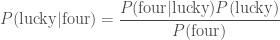
to mean the probability of A. A joint probability describes the probability of two (or more things), so we have P(A, B) as the probability that both A and B happen. The probability that A happens given that B happens is the conditional probability P(A|B). Consider the the joint probability of A and B: we want both to happen. We could construct this in a couple of ways. First we could imagine that A happens, and then B. In this case we build up the joint probability of both by working out the probability that A happens and then the probability B happens given A. Putting that in equation form

P(A,B) = P(A)P(B|A).

Alternatively, we could have B first and then A. This gives us a similar result of

P(A,B) = P(B)P(A|B).

Both of our equations give the same result. (We’ve checked this before). If we put the two together then

P(B|A)P(A) = P(A|B)P(B).

Now we divide both sides by P(A) and bam:

\displaystyle P(B|A) = \frac{P(A|B)P(B)}{P(A)},

this is Bayes’ theorem. I think the Reverend Bayes did rather well to get a theorem named after him for noting something that is true and then rearranging! We use Bayes’ theorem to update our probabilities.

Usually, when doing inference (when trying to learn from some evidence), we have some data (that our office-mate is damp) and we want to work out the probability of our hypothesis (that it’s raining). We want to calculate P(\mathrm{hypothesis}|\mathrm{data}). We normally have a model that can predict how likely it would be to observe that data if our hypothesis is true, so we know P(\mathrm{data}|\mathrm{hypothesis}), so we just need to convert between the two. This is known as the inverse problem.
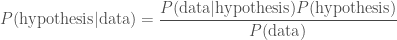
We can do this using Bayes’ theorem

\displaystyle P(\mathrm{hypothesis}|\mathrm{data}) = \frac{P(\mathrm{data}|\mathrm{hypothesis})P(\mathrm{hypothesis})}{P(\mathrm{data})}.

In this context, we give names to each of the probabilities (to make things sound extra fancy): P(\mathrm{hypothesis}|\mathrm{data}) is the posterior, because it’s what we get at the end; P(\mathrm{data}|\mathrm{hypothesis}) is the likelihood, it’s what you may remember calculating in statistics classes; P(\mathrm{hypothesis}) is the prior, because it’s what we believed about our hypothesis before we got the data, and P(\mathrm{data}) is the evidence. If ever you hear of someone doing something in a Bayesian way, it just means they are using the formula above. I think it’s rather silly to point this out, as it’s really the only logical way to do science, but people like to put “Bayesian” in the title of their papers as it sounds cool.

Whenever you get some new information, some new data, you should update your belief in your hypothesis using the above. The prior is what you believed about hypothesis before, and the posterior is what you believe after (you’ll use this posterior as your prior next time you learn something new). There are a couple of examples below, but before we get there I will take a moment to discuss priors.

About priors: what we already know

There have been many philosophical arguments about the use of priors in science. People worry that what you believe affects the results of science. Surely science should be above such things: it should be about truth, and should not be subjective! Sadly, this is not the case. Using Bayes’ theorem is the only logical thing to do. You can’t calculate a probability of what you believe after you get some data unless you know what you believed beforehand. If this makes you unhappy, just remember that when we changed our probability for it being raining outside, it didn’t change whether it was raining or not. If two different people use two different priors they can get two different results, but that’s OK, because they know different things, and so they should expect different things to happen.

To try to convince yourself that priors are necessary, consider the case that you are Sherlock Holmes (one of the modern versions), and you are trying to solve a bank robbery. There is a witness who saw the getaway, and they can remember what they saw with 99% accuracy (this gives the likelihood). If they say the getaway vehicle was a white transit van, do you believe them? What if they say it was a blue unicorn? In both cases the witness is the same, the likelihood is the same, but one is much more believable than the other. My prior that the getaway vehicle is a transit van is much greater than my prior for a blue unicorn: the latter can’t carry nearly as many bags of loot, and so is a silly choice.

If you find that changing your prior (to something else sensible) significantly changes your results, this just means that your data don’t tell you much. Imagine that you checked the weather forecast before leaving the office and it said “cloudy with 0–100% chance of precipitation”. You basically believe the same thing before and after. This really means that you need more (or better) data. I’ll talk about some good ways of calculating priors in the future.

Solving the inverse problem

Example 1: Doughnut allergy

We shall now attempt to use Bayes’ theorem to calculate some posterior probabilities. First, let’s consider a worrying situation. Imagine there is a rare genetic disease that makes you allergic to doughnuts. One in a million people have this disease, that only manifests later in life. You have tested positive. The test is 99% successful at detecting the disease if it is present, and returns a false positive (when you don’t have the disease) 1% of the time. How worried should you be? Let’s work out the probability of having the disease given that you tested positive

\displaystyle P(\mathrm{allergy}|\mathrm{positive}) = \frac{P(\mathrm{positive}|\mathrm{allergy})P(\mathrm{allergy})}{P(\mathrm{positive})}.

Our prior for having the disease is given by how common it is, P(\mathrm{allergy}) = 10^{-6}. The prior probability of not having the disease is P(\mathrm{no\: allergy}) = 1 - P(\mathrm{allergy}). The likelihood of our positive result is P(\mathrm{positive}|\mathrm{allergy}) = 0.99, which seems worrying. The evidence, the total probability of testing positive P(\mathrm{positive}) is found by adding the probability of a true positive and a false positive

 P(\mathrm{positive}) = P(\mathrm{positive}|\mathrm{allergy})P(\mathrm{allergy}) + P(\mathrm{positive}|\mathrm{no\: allergy})P(\mathrm{no\: allergy}).

The probability of a false positive is P(\mathrm{positive}|\mathrm{no\: allergy}) = 0.01. We thus have everything we need. Substituting everything in, gives

\displaystyle P(\mathrm{allergy}|\mathrm{positive}) = \frac{0.99 \times 10^{-6}}{0.99 \times 10^{-6} + 0.01 \times (1 - 10^{-6})} = 9.899 \times 10^{-5}.

Even after testing positive, you still only have about a one in ten thousand chance of having the allergy. While it is more likely that you have the allergy than a random member of the public, it’s still overwhelmingly probable that you’ll be fine continuing to eat doughnuts. Hurray!

Doughnut love

Doughnut love: probably fine.

Example 2: Boys, girls and water balloons

Second, imagine that Iris has three children. You know she has a boy and a girl, but you don’t know if she has two boys or two girls. You pop around for doughnuts one afternoon, and a girl opens the door. She is holding a large water balloon. What’s the probability that Iris has two girls? We want to calculate the posterior

\displaystyle P(\mathrm{two\: girls}|\mathrm{girl\:at\:door}) = \frac{P(\mathrm{girl\:at\:door}|\mathrm{two\: girls})P(\mathrm{two\: girls})}{P(\mathrm{girl\:at\:door})}.

As a prior, we’d expect boys and girls to be equally common, so P(\mathrm{two\: girls}) = P(\mathrm{two\: boys}) = 1/2. If we assume that it is equally likely that any one of the children opened the door, then the likelihood that one of the girls did so when their are two of them is P(\mathrm{girl\:at\:door}|\mathrm{two\: girls}) = 2/3. Similarly, if there were two boys, the probability of a girl answering the door is P(\mathrm{girl\:at\:door}|\mathrm{two\: boys}) = 1/3. The evidence, the total probability of a girl being at the door is

P(\mathrm{girl\:at\:door}) =P(\mathrm{girl\:at\:door}|\mathrm{two\: girls})P(\mathrm{two\: girls}) +P(\mathrm{girl\:at\:door}|\mathrm{two\: boys}) P(\mathrm{two\: boys}).

Using all of these,

\displaystyle P(\mathrm{two\: girls}|\mathrm{girl\:at\:door}) = \frac{(2/3)(1/2)}{(2/3)(1/2) + (1/3)(1/2)} = \frac{2}{3}.

Even though we already knew there was at least one girl, seeing a girl first makes it much more likely that the Iris has two daughters. Whether or not you end up soaked is a different question.

Example 3: Fudge!

Finally, we shall return to the case of Ted and his overconsumption of fudge. Ted claims to have eaten a lethal dose of fudge. Given that he is alive to tell the anecdote, what is the probability that he actually ate the fudge? Here, our data is that Ted is alive, and our hypothesis is that he did eat the fudge. We have

\displaystyle P(\mathrm{fudge}|\mathrm{survive}) = \frac{P(\mathrm{survive}|\mathrm{fudge})P(\mathrm{fudge})}{P(\mathrm{survive})}.

This is a case where our prior, the probability that he would eat a lethal dose of fudge P(\mathrm{fudge}), makes a difference. We know the probability of surviving the fatal dose is P(\mathrm{survive}|\mathrm{fudge}) = 0.5. The evidence, the total probability of surviving P(\mathrm{survive}),  is calculated by considering the two possible sequence of events: either Ted ate the fudge and survived or he didn’t eat the fudge and survived

P(\mathrm{survive}) = P(\mathrm{survive}|\mathrm{fudge})P(\mathrm{fudge}) + P(\mathrm{survive}|\mathrm{no\: fudge})P(\mathrm{no\: fudge}).

We’ll assume if he didn’t eat the fudge he is guaranteed to be alive, P(\mathrm{survive}| \mathrm{no\: fudge}) = 1. Since Ted either ate the fudge or he didn’t P(\mathrm{fudge}) + P(\mathrm{no\: fudge}) = 1. Therefore,

P(\mathrm{survive}) = 0.5 P(\mathrm{fudge}) + [1 - P(\mathrm{fudge})] = 1 - 0.5 P(\mathrm{fudge}).

This gives us a posterior

\displaystyle P(\mathrm{fudge}|\mathrm{survive}) = \frac{0.5 P(\mathrm{fudge})}{1 - 0.5 P(\mathrm{fudge})}.

We just need to decide on a suitable prior.

If we believe Ted could never possibly lie, then he must have eaten that fudge and P(\mathrm{fudge}) = 1. In this case,

\displaystyle P(\mathrm{fudge}|\mathrm{survive}) = \frac{0.5}{1 - 0.5} = 1.

Since we started being absolutely sure, we end up being absolutely sure: nothing could have changed our mind! This is a poor prior: it is too strong, we are being closed-minded. If you are closed-minded you can never learn anything new.

If we don’t know who Ted is, what fudge is, or the ease of consuming a lethal dose, then we might assume an equal prior on eating the fudge and not eating the fudge, P(\mathrm{fudge}) = 0.5. In this case we are in a state of ignorance. Our posterior is

\displaystyle P(\mathrm{fudge}|\mathrm{survive}) = \frac{0.5 \times 0.5}{1 - 0.5 \times 0.5} = \frac{1}{3}.

 Even though we know nothing, we conclude that it’s more probable that the Ted did not eat the fudge. In fact, it’s twice as probable that he didn’t eat the fudge than he did as P(\mathrm{no\: fudge}|\mathrm{survive}) = 1 -P(\mathrm{fudge}|\mathrm{survive}) = 2/3.

In reality, I think that it’s extremely improbable anyone could consume a lethal dose of fudge. I’m fairly certain that your body tries to protect you from such stupidity by expelling the fudge from your system before such a point. However, I will concede that it is not impossible. I want to assign a small probability to P(\mathrm{fudge}). I don’t know if this should be one in a thousand, one in a million or one in a billion, but let’s just say it is some small value p. Then

\displaystyle P(\mathrm{fudge}|\mathrm{survive}) = \frac{0.5 p}{1 - 0.5 p} \approx 0.5 p.

as the denominator is approximately one. Whatever small probability I pick, it is half as probable that Ted ate the fudge.

Mr. Impossible

I would assign a much higher probability to Mr. Impossible being able to eat that much fudge than Ted.

While it might not be too satisfying that we can’t come up with incontrovertible proof that Ted didn’t eat the fudge, we might be able to shut him up by telling him that even someone who knows nothing would think his story is unlikely, and that we will need much stronger evidence before we can overcome our prior.

Homework example: Monty Hall

You now have all the tools necessary to tackle the Monty Hall problem, one of the most famous probability puzzles:

You are on a game show and are given the choice of three doors. Behind one is a car (a Lincoln Continental), but behind the others are goats (which you don’t want). You pick a door. The host, who knows what is behind the doors, opens another door to reveal goat. They then offer you the chance to switch doors. Should you stick with your current door or not? — Monty Hall problem

You should be able to work out the probability of winning the prize by switching and sticking. You can’t guarantee you win, but you can maximise your chances.

Summary

Whenever you encounter new evidence, you should revise how probable you think things are. This is true in science, where we perform experiments to test hypotheses; it is true when trying to solve a mystery using evidence, or trying to avoid getting a goat on a game show. Bayes’ theorem is used to update probabilities. Although Bayes’ theorem itself is quite simple, calculating likelihoods, priors and evidences for use in it can be difficult. I hope to return to all these topics in the future.

How big is a black hole?

Physicist love things that are simple. This may be one of the reasons that I think black holes are cool.

Black holes form when you have something so dense that nothing can resist its own gravity: it collapses down becoming smaller and smaller. Whatever formerly made up your object (usually, the remains of what made up a star), is crushed out of existence. It becomes infinitely compact, squeezed into an infinitely small space, such that you can say that the whatever was there no longer exists. Black holes aren’t made of anything: they are just empty spacetime!

A spherical cow

Daisy, a spherical cow, or “moo-on”. Spherical cows are highly prized as pets amongst physicists because of their high degree of symmetry and ability to survive in a vacuum. They also produce delicious milkshakes.

Black holes are very simple because they are just vacuum. They are much simpler than tables, or mugs of coffee, or even spherical cows, which are all made up of things: molecules and atoms and other particles all wibbling about and interacting with each other. If you’re a fan of Game of Thrones, then you know the plot is rather complicated because there are a lot of characters. However, in a single glass of water there may be 1025 molecules: imagine how involved things can be with that many things bouncing around, occasionally evaporating, or plotting to take over the Iron Throne and rust it to pieces! Even George R. R. Martin would struggle to kill off 1025 characters. Black holes have no internal parts, they have no microstructure, they are just… nothing…

(In case you’re the type of person to worry about such things, this might not quite be true in a quantum theory, but I’m just treating them classically here.)

Since black holes aren’t made of anything, they don’t have a surface. There is no boundary, no crispy sugar shell, no transition from space to something else. This makes it difficult to really talk about the size of black holes: it is a question I often get asked when giving public talks. Black holes are really infinitely small if we just consider the point that everything collapsed to, but that’s not too useful. When we want to consider a size for a black hole, we normally use its event horizon.

Point of no return sign

The event horizon is not actually sign-posted. It’s not possible to fix a sign-post in empty space, and it would be sucked into the black hole. The sign would disappear faster than a Ramsay Street sign during a tour of the Neighbours set.

The event horizon is the point of no return. Once passed, the black hole’s gravity is inescapable; there’s no way out, even if you were able to travel at the speed of light (this is what makes them black holes). The event horizon separates the parts of the Universe where you can happily wander around from those where you’re trapped plunging towards the centre of the black hole. It is, therefore, a sensible measure of the extent of a black hole: it marks the region where the black hole’s gravity has absolute dominion (which is better than possessing the Iron Throne, and possibly even dragons).

The size of the event horizon depends upon the mass of the black hole. More massive black holes have stronger gravity, so there event horizon extends further. You need to stay further away from bigger black holes!

If we were to consider the simplest type of black hole, it’s relatively (pun intended) easy to work out where the event horizon is. The event horizon is a spherical surface, with radius

\displaystyle r_\mathrm{S} = \frac{2GM}{c^2},

This is known as the Schwarzschild radius, as this type of black hole was first theorised by Karl Schwarszchild (who was a real hard-core physicist). In this formula, M is the black hole’s mass (as it increases, so does the size of the event horizon); G is Newton’s gravitational constant (it sets the strength of gravity), and c is the speed of light (the same as in the infamous E = mc^2). You can plug in some numbers to this formula (if anything like me, two or three times before getting the correct answer), to find out how big a black hole is (or equivalently, how much you need to squeeze something before it will collapse to a black hole).

What I find shocking is that black holes are tiny! I meant it, they’re really small. The Earth has a Schwarzschild radius of 9 mm, which means you could easily lose it down the back of the sofa. Until it promptly swallowed your sofa, of course. Stellar-mass black holes are just a few kilometres across. For comparison, the Sun has a radius of about 700,000 km. For the massive black hole at the centre of our Galaxy, it is 1010 m, which does sound a lot until you release that it’s less than 10% of Earth’s orbital radius, and it’s about four million solar masses squeezed into that space.

The event horizon changes shape if the black hole has angular momentum (if it is spinning). In this case, you can get closer in, but the position of the horizon doesn’t change much. In the most extreme case, the event horizon is at a radius of

\displaystyle r_\mathrm{g} = \frac{GM}{c^2}.

Relativists like this formula, since it’s even simpler than for the Schwarzscild radius (we don’t have to remember the value of two), and it’s often called the gravitational radius. It sets the scale in relativity problems, so computer simulations often use it as a unit instead of metres or light-years or parsecs or any of the other units astronomy students despair over learning.

We’ve now figured out a sensible means of defining the size of a black hole: we can use the event horizon (which separates the part of the Universe where you can escape form the black hole, from that where there is no escape), and the size of this is around the gravitational radius r_\mathrm{g}. An interesting consequence of this (well, something I think is interesting), is to consider the effective density of a black hole. Density is how much mass you can fit into a given space. In our case, we’ll consider the mass of the black hole and the volume of its event horizon. This would be something like

\displaystyle \rho = \frac{3 M}{4 \pi r_\mathrm{g}^3} = \frac{3 c^6}{4 \pi G^3 M^2},

where I’ve used \rho for density and you shouldn’t worry about the factors of \pi or G or c, I’ve just put them in case you were curious. The interesting result is that the density decreases as the mass increases. More massive black holes are less dense! In fact, the most massive black holes, about a billion times the mass of our Sun, are less dense than water. They would float if you could find a big enough bath tub, and could somehow fill it without the water collapsing down to a black hole under its own weight…

In general, it probably makes a lot more sense (and doesn’t break the laws of physics), if you stick with a rubber duck, rather than a black hole, as a bath-time toy.

In conclusion, black holes might be smaller (and less dense) than you’d expect. However, this doesn’t mean that they’re not very dangerous. As Tyrion Lannister has shown, it doesn’t pay to judge someone by their size alone.

An introduction to probability: Great expectations

We use probabilities a lot in science. Previously, I introduced the concept of probabilities, here I’ll explain the concept of expectation and averages. Expectation and average values are one of the most useful statistics that we can construct from a probability distribution. This post contains a traces of calculus, but is peanut free.

Expectations

Imagine that we have a discrete set of numeric outcomes, such as the number from rolling a die. We’ll label these as x_1, x_2, etc., or as x_i where the subscript i is used as shorthand to indicate any of the possible outcomes. The probability of the numeric value being a particular x_i is given by P(x_i). For rolling our dice, the outcomes are one to six (x_1 =1, x_2 = 2, etc.) and the probabilities are

\displaystyle P(1) = P(2) = P(3) = P(4) = P(5) = P(6) = \frac{1}{6}.

The expectation value is the sum of all the possible outcomes multiplied by their respective probabilities,

\displaystyle \langle x \rangle = \sum_i x_i P(x_i),

where \sum_i means sum over all values of i (over all outcomes). The expectation value for rolling a die is

\displaystyle \langle x \rangle = 1 \times P(1) + 2 \times P(2) + 3 \times P(3) + 4 \times P(4) + 5 \times P(5) + 6 \times P(6) = \frac{7}{2} .

The expectation value of a distribution is its average, the value you’d expect after many (infinite) repetitions. (Of course this is possible in reality—you’d certainly get RSI—but it is useful for keeping statisticians out of mischief).

For a continuous distribution, the expectation value is given by

\displaystyle \langle x \rangle = \int x p(x) \, \mathrm{d} x ,

where p(x) is the probability density function.

You can use the expectation value to guide predictions for the outcome. You can never predict with complete accuracy (unless there is only one possible outcome), but you can use knowledge of the probabilities of the various outcomes the inform your predictions.

Imagine that after buying a large quantity of fudge, for entirely innocent reasons, the owner offers you the chance to play double-or-nothing—you’ll either pay double the bill or nothing, based on some random event—should you play?  Obviously, this depends upon the probability of winning. Let’s say that the probability of winning is p and find out how high it needs to be to be worthwhile. We can use the expectation value to calculate how much we should expect to pay, if this is less than the bill as it stands, it’s worth giving it a go, if the expectation value is larger than the original bill, we should expect to pay more (and so probably shouldn’t play). The expectation value is

\displaystyle \langle x \rangle = 0 \times (1 - p) + 2 \times p = 2 p,

where I’m working in terms of unified fudge currency, which, shockingly, is accepted in very few shops, but has the nice property that your fudge bill is always 1. Anyhow, if \langle x \rangle is less than one, so if p < 0.5, it’s worth playing. If we were tossing a (fair) coin, we’d expect to come out even, if we had to roll a six, we’d expect to pay more.

The expectation value is the equivalent of the mean. This is the average that people usually think of first. If you have a set of numeric results, you calculate the mean by adding up all or your results and dividing by the total number of results N. Imagine each outcome x_i occurs n_i times, then the mean is

\displaystyle \bar{x} = \sum_i x_i \frac{n_i}{N}.

We can estimate the probability of each outcome as P(x_i) = n_i/N so that \bar{x} = \langle x \rangle.

Median and mode

Aside from the mean there are two other commonly used averages, the median and the mode. These aren’t quite as commonly used, despite sounding friendlier. With a set of numeric results, the median is the middle result and the mode is the most common result. We can define equivalents for both when dealing with probability distributions.

To calculate the median we find the value where the total probability of being smaller (or bigger) than it is a half: P(x < x_\mathrm{med}) = 0.5. This can be done by adding up probabilities until you get a half

\displaystyle \sum_{x_i \, \leq \, x_\mathrm{med} } P(x_i) = 0.5.

For a continuous distribution this becomes

\displaystyle \int_{x_\mathrm{low}}^{x_\mathrm{med}} p(x) \, \mathrm{d}x = 0.5,

where x_\mathrm{low} is the lower limit of the distribution. (That’s all the calculus out of the way now, so if you’re not a fan you can relax). The LD50 lethal dose is a median. The median is effectively the middle of the distribution, the point at which you’re equally likely to be higher or lower.

The median is often used as it is not as sensitive as the mean to a few outlying results which are far from the typical values.

The mode is the value with the largest probability, the most probable outcome

\displaystyle P(x_\mathrm{mode}) = \max P(x_i).

For a continuous distribution, it is the point which maximises the probability density function

\displaystyle p(x_\mathrm{mode}) = \max p(x).

The modal value is the most probable outcome, the most likely result, the one to bet on if you only have one chance.

Education matters

Every so often, some official, usually an education minister, says something about wanting more than half of students to be above average. This results in much mocking, although seemingly little rise in the standards for education ministers. Having discussed averages ourselves, we can now see if it’s entirely fair to pick on these poor MPs.

The first line of defence, is that we should probably specify the distribution we’ve averaging. It may well be that they actually meant the average bear. It’s a sad truth that bears perform badly in formal education. Many blame the unfortunate stereotyping resulting from Winnie the Pooh. It might make sense to compare with performance in the past to see if standards are improving. We could imagine that taking the average from the 1400s would indeed show some improvement. For argument’s sake, let’s say that we are indeed talking about the average over this year’s students.

If the average we were talking about was the median, then it would be impossible for more (or fewer) than half of students to do better than average. In the case, it is entirely fair to mock the minister, and possibly to introduce them to the average bear. In this case, a mean bear.

If we were referring to the mode, then it is quite simple for more than half of the students to do better than this. To achieve this we just need a bottom-heavy distribution, a set of results where the most likely outcome is low, but most students do better than this. We might want to question an education system where the aim is to have a large number of students doing poorly though!

Finally, there is the mean; to use the mean, we first have to decide if we have a sensible if we are averaging a sensible quantity. For education performance this normally means exam results. Let’s sidestep the issue of if we want to reduce the output of the education system down to a single number, and consider the properties we want in order to take a sensible average. We want the results to be numeric (check); to be ordered, such that high is good and low is bad (or vice versa) so 42 is better than 41 but not as good as 43 and so on (check), and to be on a linear scale. The last criterion means that performance is directly proportional to the mark: a mark twice as big is twice as good. Most exams I’ve encountered are not like this, but I can imagine that it is possible to define a mark scheme this way. Let’s keep imagining, and assume things are sensible (and perhaps think about kittens and rainbows too… ).

We can construct a distribution where over half of students perform better than the mean. In this case we’d really need a long tail: a few students doing really very poorly. In this case, these few outliers are enough to skew the mean and make everyone else look better by comparison. This might be better than the modal case where we had a glut of students doing badly, as now we can have lots doing nicely. However, it also means that there are a few students who are totally failed by the system (perhaps growing up to become a minister for education), which is sad.

In summary, it is possible to have more than 50% of students performing above average, assuming that we are not using the median. It’s therefore unfair to heckle officials with claims of innumeracy. However, for these targets to be met requires lots of students to do badly. This seems like a poor goal. It’s probably better to try to aim for a more sensible distribution with about half of students performing above average, just like you’d expect.

On symmetry

Dave Green only combs half of his beard, the rest follows by symmetry. — Dave Green Facts

Physicists love symmetry! Using symmetry can dramatically simplify a problem. The concept of symmetry is at the heart of modern theoretical physics and some of the most beautiful of scientific results.

In this post, I’ll give a brief introduction to how physicists think about symmetry. Symmetry can be employed in a number of ways when tackling a problem; we’ll have a look at how they can help you ask the right question and then check that your answer makes sense. In a future post I hope to talk about Noether’s Theorem, my all-time favourite result in theoretical physics, which is deeply entwined with the concept of symmetry. First, we shall discuss what we mean when we talk about symmetry.

What is symmetry?

We say something is symmetric with respect to a particular operation if it is unchanged after that operation. That might sound rather generic, but that’s because the operation can be practically anything. Let’s consider a few examples:

  • Possibly the most familiar symmetry would be reflection symmetry, when something is identical to its mirror image. Something has reflection symmetry if it is invariant under switching left and right. Squares have reflection symmetry along lines in the middle of their sides and along their diagonals, rectangles only have reflection symmetry along the lines in the middle of their sides, and circles have reflection symmetry through any line that goes through their centre.
    The Star Trek Mirror Universe actually does not have reflection symmetry with our own Universe. First, they switch good and evil, rather than left and right, and second, after this transformation, we can tell the two universes apart by checking Spock’s beard.
  • Rotational symmetry is when an object is identical after being rotated. Squares are the same after a 90° rotation, rectangles are the same after a 180° rotation, and circles are the same after a rotation by any angle. There is a link between the rotational symmetry of these shapes and their mirror symmetry: you can combine two reflections to make a rotation. With rotations we have seen that symmetries can either be discrete, as for a square when we have to rotate by multiples of 90°, or continuous, as for the circle where we can pick any angle we like.
  • Translational symmetry is similar to rotational symmetry, but is when an object is the same when shifted along a particular direction. This could be a spatial direction, so shifting everything to the left, or in time. This are a little more difficult to apply to the real world than the simplified models that physicists like to imagine.
    For translational invariance, imagine an infinite, flat plane, the same in all directions. This would be translational invariant in any direction parallel to the ground. It would be a terrible place to lose your keys. If you can imagine an infinite blob of tangerine jelly, that is entirely the same in all directions, we can translate in any direction we like. We think the Universe is pretty much like this on the largest scales (where details like galaxies are no longer important), except, it’s not quite as delicious.
    The backgrounds in some Scooby-Doo cartoons show periodic translational invariance: they repeat on a loop, so if you translate by the right amount they are the same. This is a discrete symmetry, just like rotating my a fixed angle. Similarly, if you have a rigid daily routine, such that you do the same thing at the same time every day, then your schedule is symmetric with respect to a time translation of 24 hours.
  • Exchange symmetry is when you can swap two (or more) things. If you are building a LEGO model, you can switch two bricks of the same size and colour and end up with the same result, hence it is symmetric under the exchange of those bricks. The idea that we have the same physical system when we swap two particles, like two electrons, is important in quantum mechanics. In my description of translational symmetry, I could have equally well have used lime jelly instead of tangerine, or even strawberry, hence the argument is symmetric under exchange of flavours. The symmetry is destroyed should we eat the infinite jelly Universe (we might also get stomach ache).
    Mario and Luigi are not symmetric under exchange, as anyone who has tried to play multiplayer Super Mario Bros. will know, as Luigi is the better jumper and has the better moustache.

There are lots more potential symmetries. Some used by physicists seem quite obscure, such as Lorentz symmetry, but the important thing to remember is that a symmetry of a system means we get the same thing back after a transformation.

Sometimes we consider approximate symmetries, when something is almost the same under a transformation. Coke and Pepsi are approximately exchange symmetric: try switching them for yourself. They are similar, but it is possible to tell them apart. The Earth has approximate rotational symmetry, but it is not exact as it is lumpy. The spaceship at the start of Spaceballs has approximate translational invariance: it just keeps going and going, but the symmetry is not exact as it does end eventually, so the symmetry only applies to the middle.

How to use symmetry

When studying for an undergraduate degree in physics, one of the first things you come to appreciate is that some coordinate systems make problems much easier than others. Coordinates are the set of numbers that describe a position in some space. The most familiar are Cartesian coordinates, when you use x and y to describe horizontal and vertical position respectively. Cartesian coordinates give you a nice grid with everything at right-angles. Undergrad students often like to stick with Cartesian coordinates as they are straight-forward and familiar. However, they can be a pain when describing a circle. If we want to plot a line five units from the origin of of coordinate system (0,\,0), we have to solve \sqrt{x^2 + y^2} = 5. However, if we used a polar coordinate system, it would simply be r = 5. By using coordinates that match the symmetry of our system we greatly simplify the problem!

Treasure map

Pirates are trying to figure out where they buried their treasure. They know it’s 5 yarrrds from the doughnut. Calculating positions using Cartesian coordinates is difficult, but they are good for specifying specific locations, like of the palm tree.

Treasure map

Using polar coordinates, it is easy to specify the location of points 5 yarrrds from the doughnut. Pirates prefer using the polar coordinates, they really like using r.

Picking a coordinate system for a problem should depend on the symmetries of the system. If we had a system that was translation invariant, Cartesian coordinates are the best to use. If the system was invariant with respect to translation in the horizontal direction, then we know that our answer should not depend on x. If we have a system that is rotation invariant, polar coordinates are the best, as we should get an answer that doesn’t depend on the rotation angle \varphi. By understanding symmetries, we can formulate our analysis of the problem such that we ask the best questions.

At the end of my undergrad degree, my friends and I went along to an awards ceremony. I think we were hoping they’d have the miniature éclairs they normally had for special occasions. There was a chap from an evil corporation™ giving away branded clocks, that apparently ran on water. We were fairly convinced there was more to it than that, so, as now fully qualified physicists, we though we should able to figure it out. We quickly came up with two ideas: that there was some powder inside the water tank that reacted with the water to produce energy, or that the electrodes reacted in a similar way to in a potato clock. We then started to argue about how to figure this out. At this point, Peter Littlewood, then head of the Cavendish Laboratory, wandered over. We explained the problem, but not our ideas. Immediately, he said that it must be to do with the electrodes due to symmetry. Current flows to power the clock. It’ll either flow left to right through the tank, or right to left. It doesn’t matter which, but the important thing is the clock can’t have reflection symmetry. If it did, there would be no preferred direction for the current to flow. To break the symmetry, the two (similar looking) electrodes must actually be different (and hence the potato clock theory is along the right lines). My friends and I all felt appropriately impressed and humbled, but it served as a good reminder that a simple concept like symmetry can be a powerful tool.

A concept I now try to impress upon my students, is to use symmetry to guide their answers. Most are happy enough to use symmetry for error checking: if the solution is meant to have rotational symmetry and their answer depends on \varphi they know they’ve made a mistake. However, symmetry can sometimes directly tell you the answer.

Lets imagine that you’ve baked a perfectly doughnut, such that it has rotational symmetry. For some reason you sprinkled it with an even coating of electrons instead of hundreds and thousands. We now want to calculate the electric field surrounding the doughnut (for obvious reasons). The electric field tells us which way charges are pushed/pulled. We’d expect positive charges to be attracted towards our negatively charged doughnut. There should be a radial electric field to pull positive charges in, but since it has rotational symmetry, there shouldn’t be any field in the \varphi direction, as there’s now reason for charges to be pulled clockwise or anticlockwise round our doughnut. Therefore, we should be able to write down immediately that the electric field in the \varphi direction is zero, by symmetry.

Most undergrads, though, will feel that this is cheating, and will often attempt to do all the algebra (hopefully using polar coordinates). Some will get this wrong, although there might be a few who are smart enough to note that their answer must be incorrect because of the symmetry. If symmetry tells you the answer, use it! Although it is good to practise your algebra (you get better by training), you can’t learn anything more than you already knew by symmetry. Working efficiently isn’t cheating, it’s smart.

Symmetry is a useful tool for problem solving, and something that everyone should make use of.