Gravitational-wave astronomy lets us observing binary black holes. These systems, being made up of two black holes, are pretty difficult to study by any other means. It has long been argued that with this new information we can unravel the mysteries of stellar evolution. Just as a palaeontologist can discover how long-dead animals lived from their bones, we can discover how massive stars lived by studying their black hole remnants. In this paper, we quantify how much we can really learn from this black hole palaeontology—after 1000 detections, we should pin down some of the most uncertain parameters in binary evolution to a few percent precision.
Life as a binary
There are many proposed ways of making a binary black hole. The current leading contender is isolated binary evolution: start with a binary star system (most stars are in binaries or higher multiples, our lonesome Sun is a little unusual), and let the stars evolve together. Only a fraction will end with black holes close enough to merge within the age of the Universe, but these would be the sources of the signals we see with LIGO and Virgo. We consider this isolated binary scenario in this work [bonus note].
Now, you might think that with stars being so fundamentally important to astronomy, and with binary stars being so common, we’d have the evolution of binaries figured out by now. It turns out it’s actually pretty messy, so there’s lots of work to do. We consider constraining four parameters which describe the bits of binary physics which we are currently most uncertain of:
- Black hole natal kicks—the push black holes receive when they are born in supernova explosions. We now the neutron stars get kicks, but we’re less certain for black holes [bonus note].
- Common envelope efficiency—one of the most intricate bits of physics about binaries is how mass is transferred between stars. As they start exhausting their nuclear fuel they puff up, so material from the outer envelope of one star may be stripped onto the other. In the most extreme cases, a common envelope may form, where so much mass is piled onto the companion, that both stars live in a single fluffy envelope. Orbiting inside the envelope helps drag the two stars closer together, bringing them closer to merging. The efficiency determines how quickly the envelope becomes unbound, ending this phase.
- Mass loss rates during the Wolf–Rayet (not to be confused with Wolf 359) and luminous blue variable phases–stars lose mass through out their lives, but we’re not sure how much. For stars like our Sun, mass loss is low, there is enough to gives us the aurora, but it doesn’t affect the Sun much. For bigger and hotter stars, mass loss can be significant. We consider two evolutionary phases of massive stars where mass loss is high, and currently poorly known. Mass could be lost in clumps, rather than a smooth stream, making it difficult to measure or simulate.
We use parameters describing potential variations in these properties are ingredients to the COMPAS population synthesis code. This rapidly (albeit approximately) evolves a population of stellar binaries to calculate which will produce merging binary black holes.
The question is now which parameters affect our gravitational-wave measurements, and how accurately we can measure those which do?

Binary black hole merger rate at three different redshifts  as calculated by COMPAS. We show the rate in 30 different chirp mass bins for our default population parameters. The caption gives the total rate for all masses. Figure 2 of Barrett et al. (2018)
Gravitational-wave observations
For our deductions, we use two pieces of information we will get from LIGO and Virgo observations: the total number of detections, and the distributions of chirp masses. The chirp mass is a combination of the two black hole masses that is often well measured—it is the most important quantity for controlling the inspiral, so it is well measured for low mass binaries which have a long inspiral, but is less well measured for higher mass systems. In reality we’ll have much more information, so these results should be the minimum we can actually do.
We consider the population after 1000 detections. That sounds like a lot, but we should have collected this many detections after just 2 or 3 years observing at design sensitivity. Our default COMPAS model predicts 484 detections per year of observing time! Honestly, I’m a little scared about having this many signals…
For a set of population parameters (black hole natal kick, common envelope efficiency, luminous blue variable mass loss and Wolf–Rayet mass loss), COMPAS predicts the number of detections and the fraction of detections as a function of chirp mass. Using these, we can work out the probability of getting the observed number of detections and fraction of detections within different chirp mass ranges. This is the likelihood function: if a given model is correct we are more likely to get results similar to its predictions than further away, although we expect their to be some scatter.
If you like equations, the from of our likelihood is explained in this bonus note. If you don’t like equations, there’s one lurking in the paragraph below. Just remember, that it can’t see you if you don’t move. It’s OK to skip the equation.
To determine how sensitive we are to each of the population parameters, we see how the likelihood changes as we vary these. The more the likelihood changes, the easier it should be to measure that parameter. We wrap this up in terms of the Fisher information matrix. This is defined as
 ,
,
where  is the likelihood for data
  (the number of observations and their chirp mass distribution in our case),
  are our parameters (natal kick, etc.), and the angular brackets indicate the average over the population parameters. In statistics terminology, this is the variance of the score, which I think sounds cool. The Fisher information matrix nicely quantifies how much information we can lean about the parameters, including the correlations between them (so we can explore degeneracies). The inverse of the Fisher information matrix gives a lower bound on the covariance matrix (the multidemensional generalisation of the variance in a normal distribution) for the parameters . In the limit of a large number of detections, we can use the Fisher information matrix to estimate the accuracy to which we measure the parameters [bonus note].
We simulated several populations of binary black hole signals, and then calculate measurement uncertainties for our four population uncertainties to see what we could learn from these measurements.
Results
Using just the rate information, we find that we can constrain a combination of the common envelope efficiency and the Wolf–Rayet mass loss rate. Increasing the common envelope efficiency ends the common envelope phase earlier, leaving the binary further apart. Wider binaries take longer to merge, so this reduces the merger rate. Similarly, increasing the Wolf–Rayet mass loss rate leads to wider binaries and smaller black holes, which take longer to merge through gravitational-wave emission. Since the two parameters have similar effects, they are anticorrelated. We can increase one and still get the same number of detections if we decrease the other. There’s a hint of a similar correlation between the common envelope efficiency and the luminous blue variable mass loss rate too, but it’s not quite significant enough for us to be certain it’s there.
Adding in the chirp mass distribution gives us more information, and improves our measurement accuracies. The fraction uncertainties are about 2% for the two mass loss rates and the common envelope efficiency, and about 5% for the black hole natal kick. We’re less sensitive to the natal kick because the most massive black holes don’t receive a kick, and so are unaffected by the kick distribution [bonus note]. In any case, these measurements are exciting! With this type of precision, we’ll really be able to learn something about the details of binary evolution.

Measurement precision for the four population parameters after 1000 detections. We quantify the precision with the standard deviation estimated from the Fisher inforamtion matrix. We show results from 1500 realisations of the population to give an idea of scatter. Figure 5 of Barrett et al. (2018)
The accuracy of our measurements will improve (on average) with the square root of the number of gravitational-wave detections. So we can expect 1% measurements after about 4000 observations. However, we might be able to get even more improvement by combining constraints from other types of observation. Combining different types of observation can help break degeneracies. I’m looking forward to building a concordance model of binary evolution, and figuring out exactly how massive stars live their lives.
arXiv: 1711.06287 [astro-ph.HE]
Journal: Monthly Notices of the Royal Astronomical Society; 477(4):4685–4695; 2018
Favourite dinosaur: Professor Science
Bonus notes
Channel selection
In practise, we will need to worry about how binary black holes are formed, via isolated evolution or otherwise, before inferring the parameters describing binary evolution. This makes the problem more complicated. Some parameters, like mass loss rates or black hole natal kicks, might be common across multiple channels, while others are not. There are a number of ways we might be able to tell different formation mechanisms apart, such as by using spin measurements.
Kick distribution
We model the supernova kicks  as following a Maxwell–Boltzmann distribution,
 ,
,
where  is the unknown population parameter. The natal kick received by the black hole
  is not the same as this, however, as we assume some of the material ejected by the supernova falls back, reducing the over kick. The final natal kick is
 ,
,
where  is the fraction that falls back, taken from Fryer et al. (2012). The fraction is greater for larger black holes, so the biggest black holes get no kicks. This means that the largest black holes are unaffected by the value of .
The likelihood
In this analysis, we have two pieces of information: the number of detections, and the chirp masses of the detections. The first is easy to summarise with a single number. The second is more complicated, and we consider the fraction of events within different chirp mass bins.
Our COMPAS model predicts the merger rate  and the probability of falling in each chirp mass bin
  (we factor measurement uncertainty into this). Our observations are the the total number of detections
  and the number in each chirp mass bin
  (
( ). The likelihood is the probability of these observations given the model predictions. We can split the likelihood into two pieces, one for the rate, and one for the chirp mass distribution,
 .
.
For the rate likelihood, we need the probability of observing given the predicted rate . This is given by a Poisson distribution,
 ,
,
where  is the total observing time. For the chirp mass likelihood, we the probability of getting a number of detections in each bin, given the predicted fractions. This is given by a multinomial distribution,
 .
.
These look a little messy, but they simplify when you take the logarithm, as we need to do for the Fisher information matrix.
When we substitute in our likelihood into the expression for the Fisher information matrix, we get
![\displaystyle F_{ij} = \mu t_\mathrm{obs} \left[ \frac{1}{\mu^2} \frac{\partial \mu}{\partial \lambda_i} \frac{\partial \mu}{\partial \lambda_j} + \sum_k\frac{1}{p_k} \frac{\partial p_k}{\partial \lambda_i} \frac{\partial p_k}{\partial \lambda_j} \right]](https://s0.wp.com/latex.php?latex=%5Cdisplaystyle+F_%7Bij%7D+%3D+%5Cmu+t_%5Cmathrm%7Bobs%7D+%5Cleft%5B+%5Cfrac%7B1%7D%7B%5Cmu%5E2%7D+%5Cfrac%7B%5Cpartial+%5Cmu%7D%7B%5Cpartial+%5Clambda_i%7D%C2%A0%5Cfrac%7B%5Cpartial+%5Cmu%7D%7B%5Cpartial+%5Clambda_j%7D%C2%A0+%2B+%5Csum_k%5Cfrac%7B1%7D%7Bp_k%7D+%5Cfrac%7B%5Cpartial+p_k%7D%7B%5Cpartial+%5Clambda_i%7D%C2%A0%5Cfrac%7B%5Cpartial+p_k%7D%7B%5Cpartial+%5Clambda_j%7D+%5Cright%5D&bg=ffffff&fg=444444&s=0&c=20201002) .
.
Conveniently, although we only need to evaluate first-order derivatives, even though the Fisher information matrix is defined in terms of second derivatives. The expected number of events is  . Therefore, we can see that the measurement uncertainty defined by the inverse of the Fisher information matrix, scales on average as
  .
.
For anyone worrying about using the likelihood rather than the posterior for these estimates, the high number of detections [bonus note] should mean that the information we’ve gained from the data overwhelms our prior, meaning that the shape of the posterior is dictated by the shape of the likelihood.
Interpretation of the Fisher information matrix
As an alternative way of looking at the Fisher information matrix, we can consider the shape of the likelihood close to its peak. Around the maximum likelihood point, the first-order derivatives of the likelihood with respect to the population parameters is zero (otherwise it wouldn’t be the maximum). The maximum likelihood values of  and
and  are the same as their expectation values. The second-order derivatives are given by the expression we have worked out for the Fisher information matrix. Therefore, in the region around the maximum likelihood point, the Fisher information matrix encodes all the relevant information about the shape of the likelihood.
So long as we are working close to the maximum likelihood point, we can approximate the distribution as a multidimensional normal distribution with its covariance matrix determined by the inverse of the Fisher information matrix. Our results for the measurement uncertainties are made subject to this approximation (which we did check was OK).
Approximating the likelihood this way should be safe in the limit of large . As we get more detections, statistical uncertainties should reduce, with the peak of the distribution homing in on the maximum likelihood value, and its width narrowing. If you take the limit of  , you’ll see that the distribution basically becomes a delta function at the maximum likelihood values. To check that our
  was large enough, we verified that higher-order derivatives were still small.
Michele Vallisneri has a good paper looking at using the Fisher information matrix for gravitational wave parameter estimation (rather than our problem of binary population synthesis). There is a good discussion of its range of validity. The high signal-to-noise ratio limit for gravitational wave signals corresponds to our high number of detections limit.


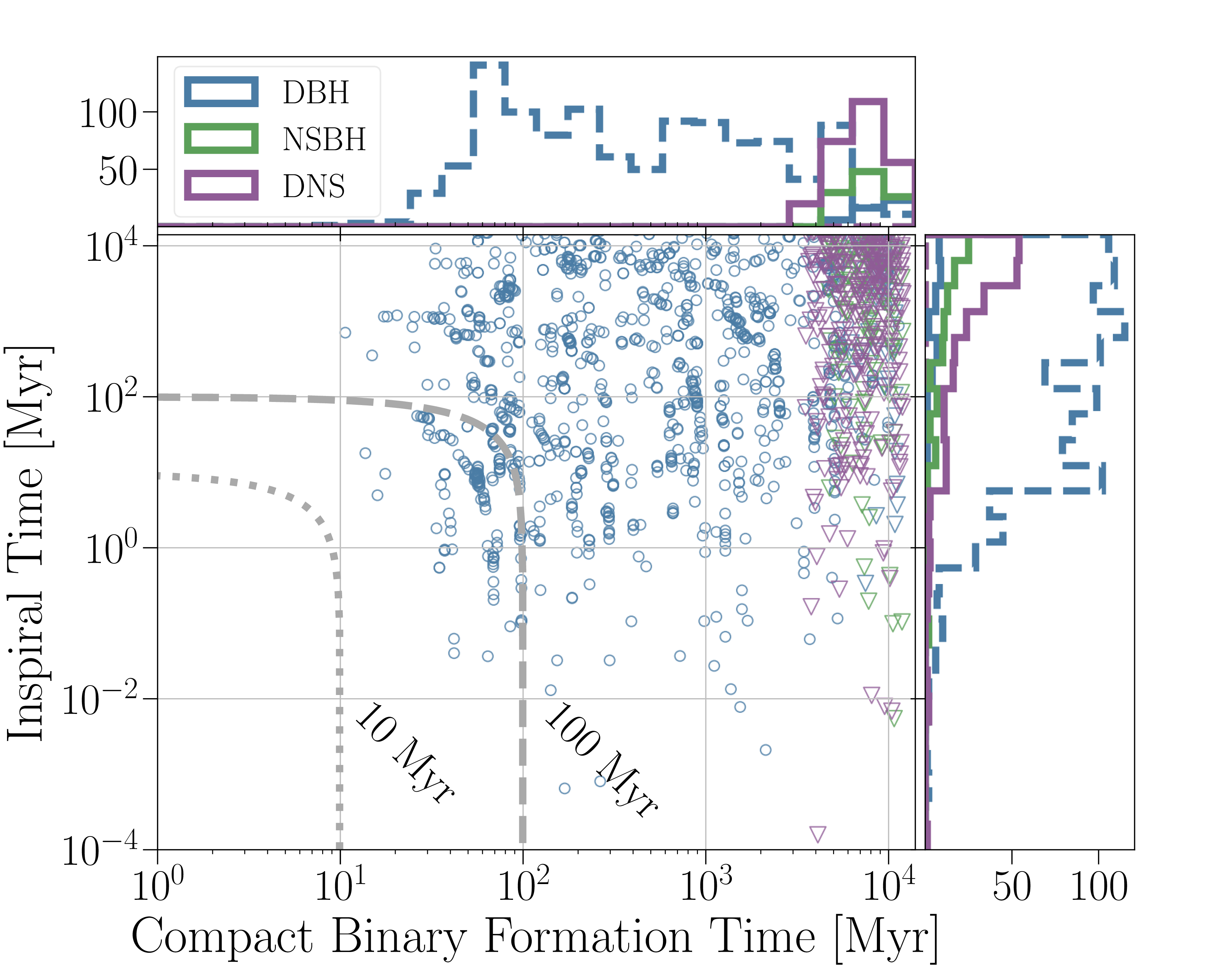

 vs inspiral time
  , and orbital separation
  vs eccentricity
  ) for our population models. The lines in the left-hand plots show the bounds for a binary to enrich a cluster of a given
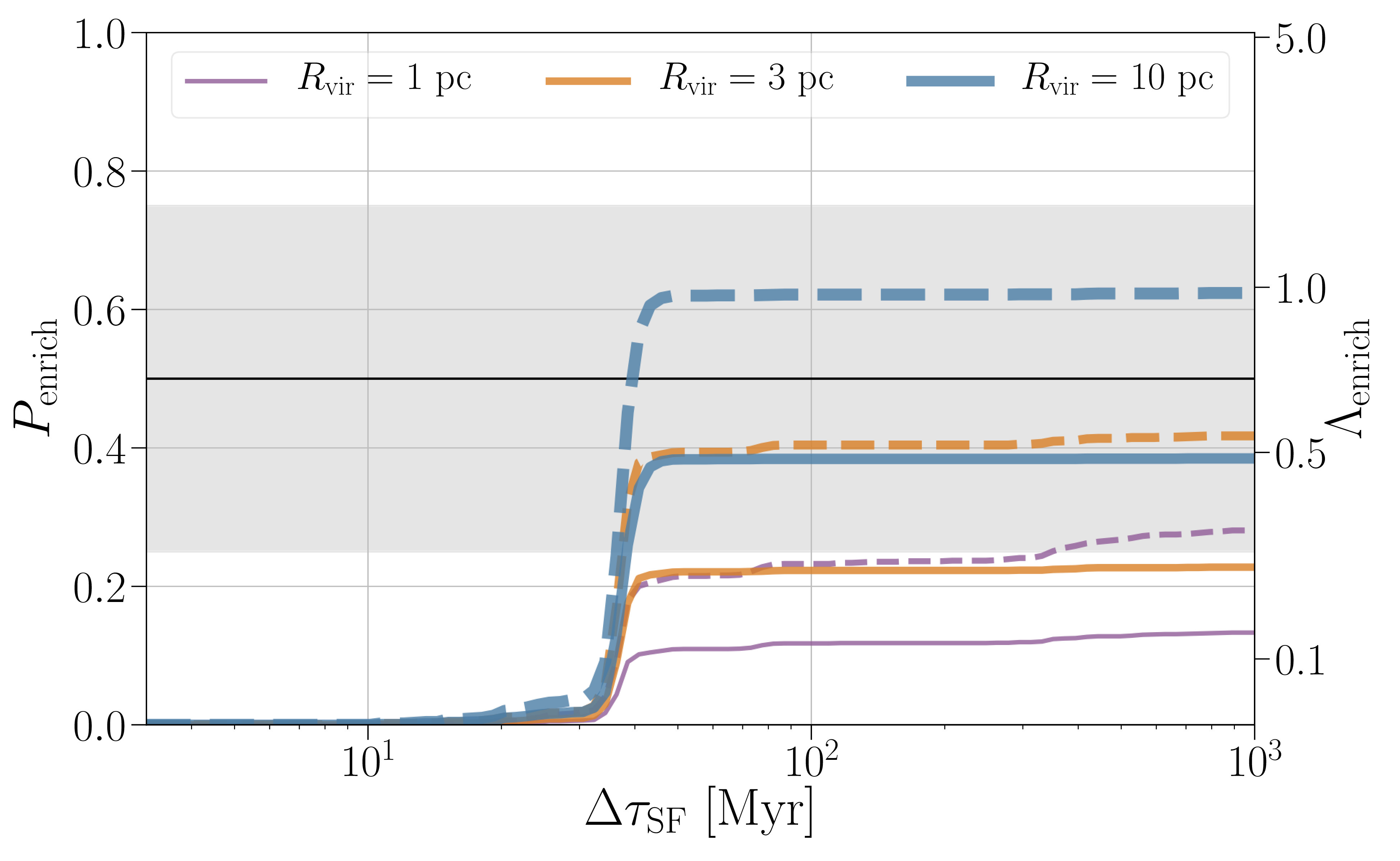
 and number of enriching binary neutron star mergers per cluster
  as a function of the timescale of star formation
  . Dashed lines are used of a cluster of a million solar masses and solid lines are used for a cluster of half this mass. Results are shown for Model D. The build up happens around the same time in different models. Figure 5 in


 binary out to a redshift of about
  . The planned detector upgrade
  . That’s pretty impressive, it means we’re covering 10 billion years of history. However, the peak in the Universe’s star formation happens at around
  when the Universe was only 200 million years old and the first stars light up.
 we need this low frequency sensitivity. At the moment, Advanced LIGO could get down to about
  . The plot below shows the signal from a
  binary at
  . The signal is completely undetectable at
 . If the questions can be answered with
  , then we don’t need anything beyond the currently planned A+. If we need a slightly larger
  (blue line) we can survey black holes around
  –
– across cosmic time.
 out to redshift
  . The blue curve highlights the reach at a boost factor of
  with a lower cut-off frequency of
  , we can investigate the various possibilities. The plot below shows the possible combinations of parameters which meet of requirements.

 per redshift bin as a function of A+ boost factor

 . The position is measured in terms of the
  . The
. The  . Part of Figure 1 of the

 –
– , which is about
  –
–
 –
– galaxies.


 is inversely proportional to the sixth power of the signal-to-noise ration
  . This is what you would expect. The localization volume depends upon the angular uncertainty on the sky
  , the distance to the source
  , and the distance uncertainty
  ,
, .
. .
. .
. .
.

 , the Wolf–Rayet mass loss rate
  , and the luminous blue variable mass loss rate
  . There is an anticorrealtion between
  and
and 


 . Results are shown for the different astrophysical models, and for the different signal models. The astrophysical model has little impact on the uncertainties. M4 shows a slight difference as it assumes heavier stellar-mass black holes. The results with the two signal models agree when the massive black hole is not spinning (M10 and M11). Otherwise, measurements are more precise with the AKK signal model, as this includes extra signal from the end of the inspiral. Part of Figure 11 of
 where
where  is the frequency emitted, and
  for a nearby source, and is larger for further away sources). Lower frequency gravitational waves correspond to higher mass systems, so it is often convenient to work with the redshifted mass, the mass corresponding to the signal you measure if you ignore redshifting. The redshifted mass of the massive black hole is
  where
where 
 . The signal model is not as important here, as the uncertainty only depends on how loud the signal is. Part of Figure 12 of
 . Results are similar to the mass and spin measurements. Figure 13 of
 , one for polar (north/south if we think of the spin of the massive black hole like the rotation of the Earth) motion
  and one for axial (around in the east/west direction) motion. As gravitational waves are emitted, and the orbit shrinks, these frequencies evolve. The animation above, made by
 –
– plane. Credit: Rob Cole
 which is defined below. Figure 4 of
  .
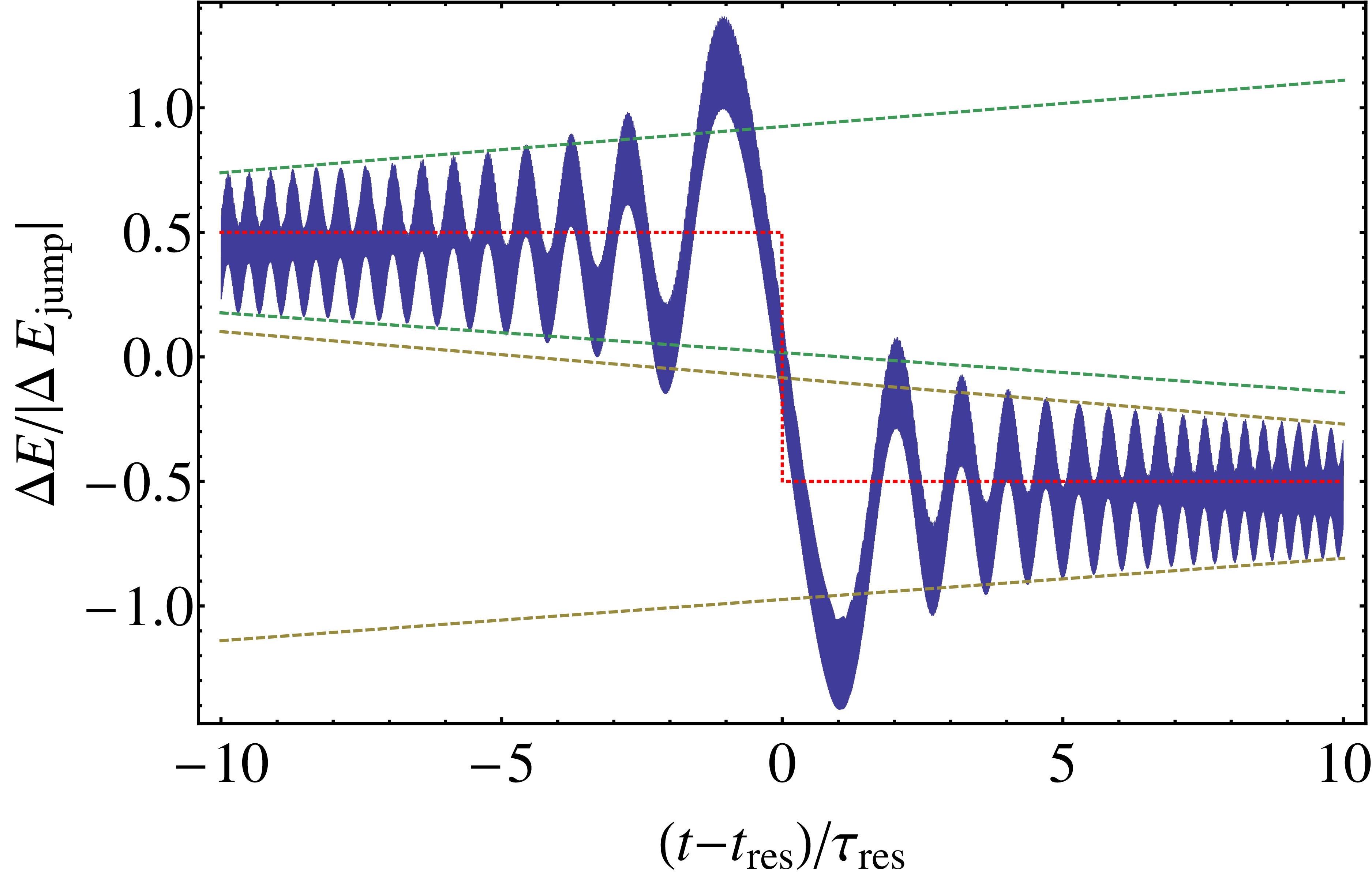
. . What should this depend on? There are three ingredients. First, the rate of change of this constant
  on the resonant orbit. Second, the time spent on resonance
  .
. . By varying
  ,
, . Now, we know the pieces, we can try to figure out what the pieces are.
 : the smaller the stellar-mass black hole is relative to the massive one, the smaller
  , which is zero exactly on resonance. If this is evolving at rate
  , then the resonance timescale is
![\displaystyle \tau_\mathrm{res} = \left[\frac{2\pi}{\dot{\Omega}}\right]^{1/2}](https://s0.wp.com/latex.php?latex=%5Cdisplaystyle+%5Ctau_%5Cmathrm%7Bres%7D+%3D+%5Cleft%5B%5Cfrac%7B2%5Cpi%7D%7B%5Cdot%7B%5COmega%7D%7D%5Cright%5D%5E%7B1%2F2%7D&bg=ffffff&fg=444444&s=0&c=20201002) .
. and the long evolution timescale
  :
: .
. , we need to do some quite involved maths (given in Appendix B of the
  and
and  ) have smaller jumps than lower-order ones. This makes sense, as higher-order resonances come closer to covering all the points in the space, and so are more like averaging over the entire space. Second, jumps are larger for higher eccentricity orbits. This also makes sense, as you can’t have resonances for circular (zero eccentricity orbits) as there’s no radial frequency, so the size of the jumps must tend to zero. We’ll see that these two points are important when it comes to observational consequences of transient resonances.
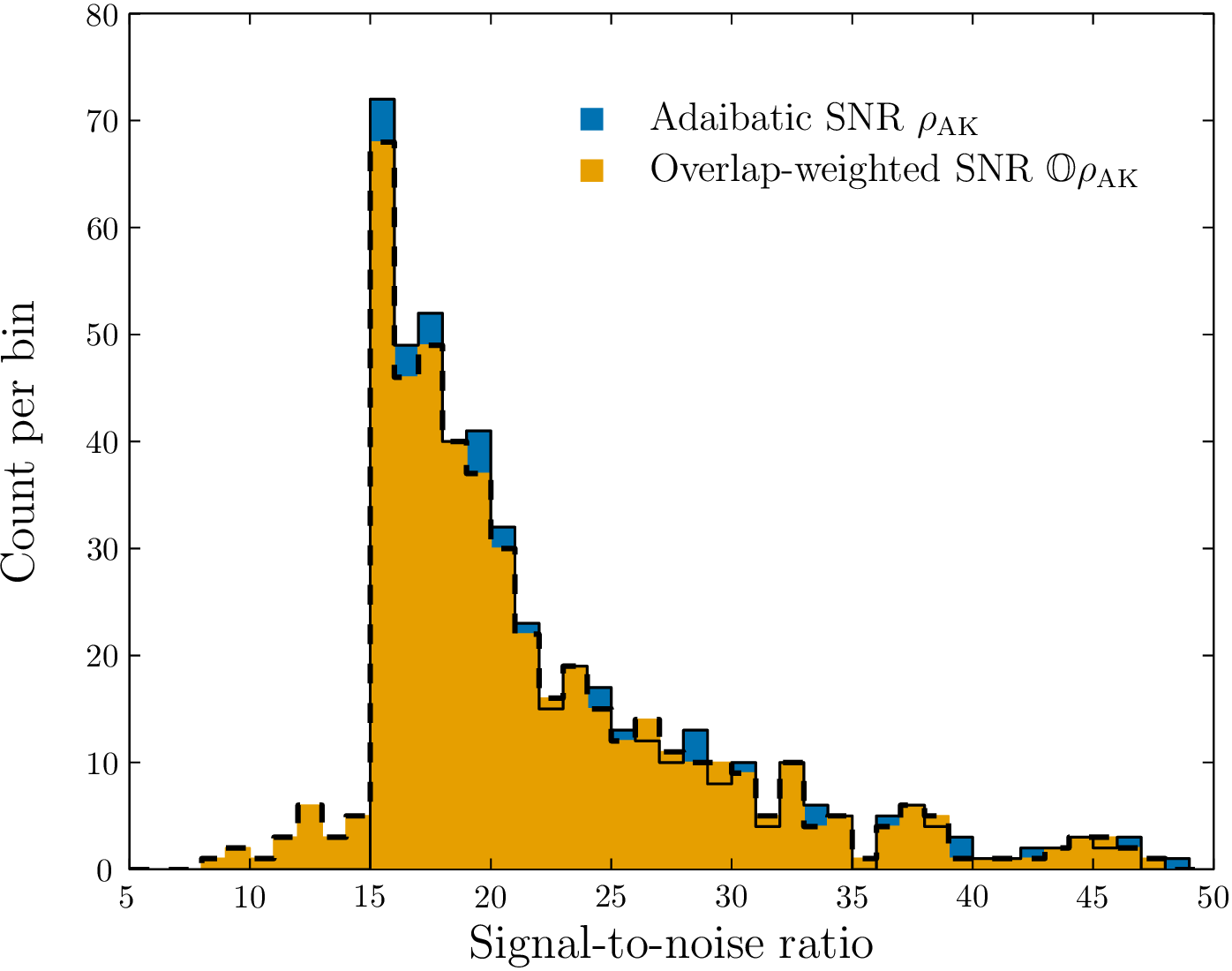
 are not important because the spacetime is axisymmetric. The equations are exactly identical for all values of the the axial angle
  , so it doesn’t matter where you are (or if you keep cycling over the same spot) for the evolution of the EMRI.
 , we want to know the probability that the parameters
  have different values, which is written as
  . This is calculated using
 ,
, is the likelihood, which we can calculate from our knowledge of the
  is the prior on the parameters (what we would have guessed before we had the data), and the normalisation constant
  is called the evidence. We’ll use the evidence again in the next layer of inference.
 ,
, denotes which model we are considering.
 , we can work this out using another application of Bayes’ theorem (yay)
 ,
, is just all the evidences for the individual events (given that model) multiplied together,
  is our prior for the different models, and
  is another normalisation constant.
