Going the distance: Mapping host galaxies of LIGO and Virgo sources in three dimensions using local cosmography and targeted follow-up

October 22, 2016August 10, 2018 / CPLB / Leave a comment

GW150914 claimed the title of many firsts—it was the first direct observation of gravitational waves, the first observation of a binary black hole system, the first observation of two black holes merging, the first time time we’ve tested general relativity in such extreme conditions… However, there are still many firsts for gravitational-wave astronomy yet to come (hopefully, some to be accompanied by cake). One of the most sought after, is the first is signal to have a clear electromagnetic counterpart—a glow in some part of the spectrum of light (from radio to gamma-rays) that we can observe with telescopes.

Identifying a counterpart is challenging, as it is difficult to accurately localise a gravitational-wave source. electromagnetic observers must cover a large area of sky before any counterparts fade. Then, if something is found, it can be hard to determine if that is from the same source as the gravitational waves, or some thing else…

To help the search, it helps to have as much information as possible about the source. Especially useful is the distance to the source. This can help you plan where to look. For nearby sources, you can cross-reference with galaxy catalogues, and perhaps pick out the biggest galaxies as the most likely locations for the source [bonus note]. Distance can also help plan your observations: you might want to start with regions of the sky where the source would be closer and so easiest to spot, or you may want to prioritise points where it is further and so you’d need to observe longer to detect it (I’m not sure there’s a best strategy, it depends on the telescope and the amount of observing time available). In this paper we describe a method to provide easy-to-use distance information, which could be supplied to observers to help their search for a counterpart.

Going the distance

This work is the first spin-off from the First 2 Years trilogy of papers, which looked a sky localization and parameter estimation for binary neutron stars in the first two observing runs of the advance-detector era. Binary neutron star coalescences are prime candidates for electromagnetic counterparts as we think there should be a bigger an explosion as they merge. I was heavily involved in the last two papers of the trilogy, but this study was led by Leo Singer: I think I mostly annoyed Leo by being a stickler when it came to writing up the results.

3D localization with the two LIGO detectors

Three-dimensional localization showing the 20%, 50%, and 90% credible levels for a typical two-detector early Advanced LIGO event. The Earth is shown at the centre, marked by $\oplus$ . The true location is marked by the cross. Leo poetically described this as looking like the seeds of the jacaranda tree, and less poetically as potato chips. Figure 1 of Singer et al. (2016).

The idea is to provide a convenient means of sharing a 3D localization for a gravitational wave source. The full probability distribution is rather complicated, but it can be made more manageable if you break it up into pixels on the sky. Since astronomers need to decide where to point their telescopes, breaking up the 3D information along different lines of sight, should be useful for them.

Each pixel covers a small region of the sky, and along each line of sight, the probability distribution for distance $D$ can be approximated using an ansatz

$\displaystyle p(D|\mathrm{data}) \propto D^2\exp\left[-\frac{(D - \mu)^2}{2\sigma}\right]$ ,

where $\mu$ and $\sigma$ are calculated for each pixel individually. The form of this ansatz can be understood as the posterior probability distribution is proportional to the product of the prior and the likelihood. Our prior is that sources are uniformly distributed in volume, which means $\propto D^2$ , and the likelihood can often be well approximated as a Gaussian distribution, which gives the other piece [bonus note].

The ansatz doesn’t always fit perfectly, but it performs well on average. Considering the catalogue of binary neutron star signals used in the earlier papers, we find that roughly 50% of the time sources are found within the 50% credible volume, 90% are found in the 90% volume, etc. We looked at a more sophisticated means of constructing the localization volume in a companion paper.

The 3D localization is easy to calculate, and Leo has worked out a cunning way to evaluate the ansatz with BAYESTAR, our rapid sky-localization code, meaning that we can produce it on minute time-scales. This means that observers should have something to work with straight-away, even if we’ll need to wait a while for the full, final results. We hope that this will improve prospects for finding counterparts—some potential examples are sketched out in the penultimate section of the paper.

If you are interested in trying out the 3D information, there is a data release and the supplement contains a handy Python tutorial. We are hoping that the Collaboration will use the format for alerts for LIGO and Virgo’s upcoming observing run (O2).

arXiv: 1603.07333 [astro-ph.HE]; 1605.04242 [astro-ph.IM]
Journal: Astrophysical Journal Letters; 829(1):L15(7); 2016; Astrophysical Journal Supplement Series; 226(1):10(8); 2016
Data release: Going the distance
Favourite crisp flavour: Salt & vinegar
Favourite jacaranda: Jacaranda mimosifolia

Bonus notes

Catalogue shopping

The Event’s source has a luminosity distance of around 250–570 Mpc. This is sufficiently distant that galaxy catalogues are incomplete and not much use when it comes to searching. GW151226 and LVT151012 have similar problems, being at around the same distance or even further.

The gravitational-wave likelihood

For the professionals interested in understanding more about the shape of the likelihood, I’d recommend Cutler & Flanagan (1994). This is a fantastic paper which contains many clever things [bonus bonus note]. This work is really the foundation of gravitational-wave parameter estimation. From it, you can see how the likelihood can be approximated as a Gaussian. The uncertainty can then be evaluated using Fisher matrices. Many studies have been done using Fisher matrices, but it important to check that this is a valid approximation, as nicely explained in Vallisneri (2008). I ran into a case when it didn’t during my PhD.

Mergin’

As a reminder that smart people make mistakes, Cutler & Flanagan have a typo in the title of arXiv posting of their paper. This is probably the most important thing to take away from this paper.

Parameter estimation on gravitational waves from neutron-star binaries with spinning components

October 1, 2016October 15, 2017 / CPLB / Leave a comment

blIn gravitation-wave astronomy, some parameters are easier to measure than others. We are sensitive to properties which change the form of the wave, but sometimes the effect of changing one parameter can be compensated by changing another. We call this a degeneracy. In signals for coalescing binaries (two black holes or neutron stars inspiralling together), there is a degeneracy between between the masses and spins. In this recently published paper, we look at what this means for observing binary neutron star systems.

History

This paper has been something of an albatross, and I’m extremely pleased that we finally got it published. I started working on it when I began my post-doc at Birmingham in 2013. Back then I was sharing an office with Ben Farr, and together with others in the Parameter Estimation Group, we were thinking about the prospect of observing binary neutron star signals (which we naively thought were the most likely) in LIGO’s first observing run.

One reason that this work took so long is that binary neutron star signals can be computationally expensive to analyse [bonus note]. The signal slowly chirps up in frequency, and can take up to a minute to sweep through the range of frequencies LIGO is sensitive to. That gives us a lot of gravitational wave to analyse. (For comparison, GW150914 lasted 0.2 seconds). We need to calculate waveforms to match to the observed signals, and these can be especially complicated when accounting for the effects of spin.

A second reason is shortly after submitting the paper in August 2015, we got a little distracted…

This paper was the third of a trilogy look at measuring the properties of binary neutron stars. I’ve written about the previous instalment before. We knew that getting the final results for binary neutron stars, including all the important effects like spin, would take a long time, so we planned to follow up any detections in stages. A probable sky location can be computed quickly, then we can have a first try at estimating other parameters like masses using waveforms that don’t include spin, then we go for the full results with spin. The quicker results would be useful for astronomers trying to find any explosions that coincided with the merger of the two neutron stars. The first two papers looked at results from the quicker analyses (especially at sky localization); in this one we check what effect neglecting spin has on measurements.

What we did

We analysed a population of 250 binary neutron star signals (these are the same as the ones used in the first paper of the trilogy). We used what was our best guess for the sensitivity of the two LIGO detectors in the first observing run (which was about right).

The simulated neutron stars all have small spins of less than 0.05 (where 0 is no spin, and 1 would be the maximum spin of a black hole). We expect neutron stars in these binaries to have spins of about this range. The maximum observed spin (for a neutron star not in a binary neutron star system) is around 0.4, and we think neutron stars should break apart for spins of 0.7. However, since we want to keep an open mind regarding neutron stars, when measuring spins we considered spins all the way up to 1.

What we found

Our results clearly showed the effect of the mass–spin degeneracy. The degeneracy increases the uncertainty for both the spins and the masses.

Even though the true spins are low, we find that across the 250 events, the median 90% upper limit on the spin of the more massive (primary) neutron star is 0.70, and the 90% limit on the less massive (secondary) neutron star is 0.86. We learn practically nothing about the spin of the secondary, but a little more about the spin of the primary, which is more important for the inspiral. Measuring spins is hard.

The effect of the mass–spin degeneracy for mass measurements is shown in the plot below. Here we show a random selection of events. The banana-shaped curves are the 90% probability intervals. They are narrow because we can measure a particular combination of masses, the chirp mass, really well. The mass–spin degeneracy determines how long the banana is. If we restrict the range of spins, we explore less of the banana (and potentially introduce an offset in our results).

Rough outlines for 90% credible regions for component masses for a random assortments of signals. The circles show the true values. The coloured lines indicate the extent of the distribution with different limits on the spins. The grey area is excluded from our convention on masses $m_1 \geq m_2$ . Figure 5 from Farr et al. (2016).

Although you can’t see it in the plot above, including spin does also increase the uncertainty in the chirp mass too. The plots below show the standard deviation (a measure width of the posterior probability distribution), divided by the mean for several mass parameters. This gives a measure of the fractional uncertainty in our measurements. We show the chirp mass $\mathcal{M}_\mathrm{c}$ , the mass ratio $q = m_2/m_1$ and the total mass 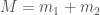$M = m_1 + m_2$ , where $m_1$ and $m_2$ are the masses of the primary and secondary neutron stars respectively. The uncertainties are small for louder signals (higher signal-to-noise ratio). If we neglect the spin, the true chirp mass can lie outside the posterior distribution, the average is about 5 standard deviations from the mean, but if we include spin, the offset is just 0.7 from the mean (there’s still some offset as we’re allowing for spins all the way up to 1).

Mass measurements for binary neutron stars with and without spin

Fractional statistical uncertainties in chirp mass (top), mass ratio (middle) and total mass (bottom) estimates as a function of network signal-to-noise ratio for both the fully spinning analysis and the quicker non-spinning analysis. The lines indicate approximate power-law trends to guide the eye. Figure 2 of Farr et al. (2016).

We need to allow for spins when measuring binary neutron star masses in order to explore for the possible range of masses.

Sky localization and distance, however, are not affected by the spins here. This might not be the case for sources which are more rapidly spinning, but assuming that binary neutron stars do have low spin, we are safe using the easier-to-calculate results. This is good news for astronomers who need to know promptly where to look for explosions.

arXiv: 1508.05336 [astro-ph.HE]
Journal: Astrophysical Journal; 825(2):116(10); 2016
Authorea [bonus note]: Parameter estimation on gravitational waves from neutron-star binaries with spinning components
Conference proceedings: Early Advanced LIGO binary neutron-star sky localization and parameter estimation
Favourite albatross: Wilbur

Bonus notes

How long?

The plot below shows how long it took to analyse each of the binary neutron star signals.

Run time for different analyses of binary neutron stars

Distribution of run times for binary neutron star signals. Low-latency sky localization is done with BAYESTAR; medium-latency non-spinning parameter estimation is done with LALInference and TaylorF2 waveforms, and high-latency fully spinning parameter estimation is done with LALInference and SpinTaylorT4 waveforms. The LALInference results are for 2000 posterior samples. Figure 9 from Farr et al. (2016).

BAYESTAR provides a rapid sky localization, taking less than ten seconds. This is handy for astronomers who want to catch a flash caused by the merger before it fades.

Estimates for the other parameters are computed with LALInference. How long this takes to run depends on which waveform you are using and how many samples from the posterior probability distribution you want (the more you have, the better you can map out the shape of the distribution). Here we show times for 2000 samples, which is enough to get a rough idea (we collected ten times more for GW150914 and friends). Collecting twice as many samples takes (roughly) twice as long. Prompt results can be obtained with a waveform that doesn’t include spin (TaylorF2), these take about a day at most.

For this work, we considered results using a waveform which included the full effects of spin (SpinTaylorT4). These take about twenty times longer than the non-spinning analyses. The maximum time was 172 days. I have a strong suspicion that the computing time cost more than my salary.

Waiting for LALInference runs to finish gives you some time to practise hobbies. This is a globe knitted by Hannah. The two LIGO sites marked in red, and a typical gravitational-wave sky localization stitched on.

In order to get these results, we had to add check-pointing to our code, so we could stop it and restart it; we encountered a new type of error in the software which manages jobs running on our clusters, and Hannah Middleton and I got several angry emails from cluster admins (who are wonderful people) for having too many jobs running.

In comparison, analysing GW150914, LVT151012 and GW151226 was a breeze. Grudgingly, I have to admit that getting everything sorted out for this study made us reasonably well prepared for the real thing. Although, I’m not looking forward to that first binary neutron star signal…

Authorea

Authorea is an online collaborative writing service. It allows people to work together on documents, editing text, adding comments, and chatting with each other. By the time we came to write up the paper, Ben was no longer in Birmingham, and many of our coauthors are scattered across the globe. Ben thought Authorea might be useful for putting together the paper.

Writing was easy, and the ability to add comments on the text was handy for getting feedback from coauthors. The chat was going for quickly sorting out issues like plots. Overall, I was quite pleased, up to the point we wanted to get the final document. Extracted a nicely formatted PDF was awkward. For this I switched to using the Github back-end. On reflection, a simple git repo, plus a couple of Skype calls might have been a smoother way of writing, at least for a standard journal article.

Authorea promises to be an open way of producing documents, and allows for others to comment on papers. I don’t know if anyone’s looked at our Authorea article. For astrophysics, most people use the arXiv, which is free to everyone, and I’m not sure if there’s enough appetite for interaction (beyond the occasional email to authors) to motivate people to look elsewhere. At least, not yet.

In conclusion, I think Authorea is a nice idea, and I would try out similar collaborative online writing tools again, but I don’t think I can give it a strong recommendation for your next paper unless you have a particular idea in mind of how to make the most of it.

Testing general relativity using golden black-hole binaries

August 27, 2016October 15, 2017 / CPLB / Leave a comment

Binary black hole mergers are the ultimate laboratory for testing gravity. The gravitational fields are strong, and things are moving at close to the speed of light. these extreme conditions are exactly where we expect our theories could breakdown, which is why we were so exciting by detecting gravitational waves from black hole coalescences. To accompany the first detection of gravitational waves, we performed several tests of Einstein’s theory of general relativity (it passed). This paper outlines the details of one of the tests, one that can be extended to include future detections to put Einstein’s theory to the toughest scrutiny.

One of the difficulties of testing general relativity is what do you compare it to? There are many alternative theories of gravity, but only a few of these have been studied thoroughly enough to give an concrete idea of what a binary black hole merger should look like. Even if general relativity comes out on top when compared to one alternative model, it doesn’t mean that another (perhaps one we’ve not thought of yet) can be ruled out. We need ways of looking for something odd, something which hints that general relativity is wrong, but doesn’t rely on any particular alternative theory of gravity.

The test suggested here is a consistency test. We split the gravitational-wave signal into two pieces, a low frequency part and a high frequency part, and then try to measure the properties of the source from the two parts. If general relativity is correct, we should get answers that agree; if it’s not, and there’s some deviation in the exact shape of the signal at different frequencies, we can get different answers. One way of thinking about this test is imagining that we have two experiments, one where we measure lower frequency gravitational waves and one where we measure higher frequencies, and we are checking to see if their results agree.

To split the waveform, we use a frequency around that of the last stable circular orbit: about the point that the black holes stop orbiting about each other and plunge together and merge [bonus note]. For GW150914, we used 132 Hz, which is about the same as the C an octave below middle C (a little before time zero in the simulation below). This cut roughly splits the waveform into the low frequency inspiral (where the two black hole are orbiting each other), and the higher frequency merger (where the two black holes become one) and ringdown (where the final black hole settles down).

We are fairly confident that we understand what goes on during the inspiral. This is similar physics to where we’ve been testing gravity before, for example by studying the orbits of the planets in the Solar System. The merger and ringdown are more uncertain, as we’ve never before probed these strong and rapidly changing gravitational fields. It therefore seems like a good idea to check the two independently [bonus note].

We use our parameter estimation codes on the two pieces to infer the properties of the source, and we compare the values for the mass $M_f$ and spin $\chi_f$ of the final black hole. We could use other sets of parameters, but this pair compactly sum up the properties of the final black hole and are easy to explain. We look at the difference between the estimated values for the mass and spin, $\Delta M_f$ and $\Delta \chi_f$ , if general relativity is a good match to the observations, then we expect everything to match up, and $\Delta M_f$ and $\Delta \chi_f$ to be consistent with zero. They won’t be exactly zero because we have noise in the detector, but hopefully zero will be within the uncertainty region [bonus note]. An illustration of the test is shown below, including one of the tests we did to show that it does spot when general relativity is not correct.

Results from the consistency test. The top panels show the outlines of the 50% and 90% credible levels for the low frequency (inspiral) part of the waveform, the high frequency (merger–ringdown) part, and the entire (inspiral–merger–ringdown, IMR) waveform. The bottom panel shows the fractional difference between the high and low frequency results. If general relativity is correct, we expect the distribution to be consistent with $(0,0)$ , indicated by the cross (+). The left panels show a general relativity simulation, and the right panel shows a waveform from a modified theory of gravity. Figure 1 of Ghosh et al. (2016).

A convenient feature of using $\Delta M_f$ and $\Delta \chi_f$ to test agreement with relativity, is that you can combine results from multiple observations. By averaging over lots of signals, you can reduce the uncertainty from noise. This allows you to pin down whether or not things really are consistent, and spot smaller deviations (we could get precision of a few percent after about 100 suitable detections). I look forward to seeing how this test performs in the future!

arXiv: 1602.02453 [gr-qc]
Journal: Physical Review D; 94(2):021101(6); 2016
Favourite golden thing: Golden syrup sponge pudding

Bonus notes

Review

I became involved in this work as a reviewer. The LIGO Scientific Collaboration is a bit of a stickler when it comes to checking its science. We had to check that the test was coded up correctly, that the results made sense, and that calculations done and written up for GW150914 were all correct. Since most of the team are based in India [bonus note], this involved some early morning telecons, but it all went smoothly.

One of our checks was that the test wasn’t sensitive to exact frequency used to split the signal. If you change the frequency cut, the results from the two sections do change. If you lower the frequency, then there’s less of the low frequency signal and the measurement uncertainties from this piece get bigger. Conversely, there’ll be more signal in the high frequency part and so we’ll make a more precise measurement of the parameters from this piece. However, the overall results where you combine the two pieces stay about the same. You get best results when there’s a roughly equal balance between the two pieces, but you don’t have to worry about getting the cut exactly on the innermost stable orbit.

Golden binaries

In order for the test to work, we need the two pieces of the waveform to both be loud enough to allow us to measure parameters using them. This type of signals are referred to as golden. Earlier work on tests of general relativity using golden binaries has been done by Hughes & Menou (2015), and Nakano, Tanaka & Nakamura (2015). GW150914 was a golden binary, but GW151226 and LVT151012 were not, which is why we didn’t repeat this test for them.

GW150914 results

For The Event, we ran this test, and the results are consistent with general relativity being correct. The plots below show the estimates for the final mass and spin (here denoted $a_f$ rather than $\chi_f$ ), and the fractional difference between the two measurements. The points $(0,0)$ is at the 28% credible level. This means that if general relativity is correct, we’d expect a deviation at this level to occur around-about 72% of the time due to noise fluctuations. It wouldn’t take a particular rare realisation of noise to cause the assume true value of $(0,0)$ to be found at this probability level, so we’re not too suspicious that something is amiss with general relativity.

Results from the consistency test for The Event. The top panels final mass and spin measurements from the low frequency (inspiral) part of the waveform, the high frequency (post-inspiral) part, and the entire (IMR) waveform. The bottom panel shows the fractional difference between the high and low frequency results. If general relativity is correct, we expect the distribution to be consistent with $(0,0)$ , indicated by the cross. Figure 3 of the Testing General Relativity Paper.

The authors

Abhirup Ghosh and Archisman Ghosh were two of the leads of this study. They are both A. Ghosh at the same institution, which caused some confusion when compiling the LIGO Scientific Collaboration author list. I think at one point one of them (they can argue which) was removed as someone thought there was a mistaken duplication. To avoid confusion, they now have their full names used. This is a rare distinction on the Discovery Paper (I’ve spotted just two others). The academic tradition of using first initials plus second name is poorly adapted to names which don’t fit the typical western template, so we should be more flexible.

Inference on gravitational waves from coalescences of stellar-mass compact objects and intermediate-mass black holes

June 4, 2016August 27, 2016 / CPLB / Leave a comment

I love collecting things, there’s something extremely satisfying about completing a set. I suspect that this is one of the alluring features of Pokémon—you’ve gotta catch ’em all. The same is true of black hole hunting. Currently, we know of stellar-mass black holes which are a few times the mass of our Sun, up to a few tens of the mass of our Sun (the black holes of GW150914 are the biggest yet to be observed), and we know of supermassive black holes, which are ten thousand to ten billion times the mass our Sun. However, we are missing intermediate-mass black holes which lie in the middle. We have Charmander and Charizard, but where is Charmeleon? The elusive ones are always the most satisfying to capture.

Adorable black hole (available for adoption). I’m sure this could be a Pokémon. It would be a Dark type. Not that I’ve given it that much thought…

Intermediate-mass black holes have evaded us so far. We’re not even sure that they exist, although that would raise questions about how you end up with the supermassive ones (you can’t just feed the stellar-mass ones lots of rare candy). Astronomers have suggested that you could spot intermediate-mass black holes in globular clusters by the impact of their gravity on the motion of other stars. However, this effect would be small, and near impossible to conclusively spot. Another way (which I’ve discussed before), would to be to look at ultra luminous X-ray sources, which could be from a disc of material spiralling into the black hole. However, it’s difficult to be certain that we understand the source properly and that we’re not misclassifying it. There could be one sure-fire way of identifying intermediate-mass black holes: gravitational waves.

The frequency of gravitational waves depend upon the mass of the binary. More massive systems produce lower frequencies. LIGO is sensitive to the right range of frequencies for stellar-mass black holes. GW150914 chirped up to the pitch of a guitar’s open B string (just below middle C). Supermassive black holes produce gravitational waves at too low frequency for LIGO (a space-based detector would be perfect for these). We might just be able to detect signals from intermediate-mass black holes with LIGO.

In a recent paper, a group of us from Birmingham looked at what we could learn from gravitational waves from the coalescence of an intermediate-mass black hole and a stellar-mass black hole [bonus note]. We considered how well you would be able to measure the masses of the black holes. After all, to confirm that you’ve found an intermediate-mass black hole, you need to be sure of its mass.

The signals are extremely short: we only can detect the last bit of the two black holes merging together and settling down as a final black hole. Therefore, you might think there’s not much information in the signal, and we won’t be able to measure the properties of the source. We found that this isn’t the case!

We considered a set of simulated signals, and analysed these with our parameter-estimation code [bonus note]. Below are a couple of plots showing the accuracy to which we can infer a couple of different mass parameters for binaries of different masses. We show the accuracy of measuring the chirp mass $\mathcal{M}$ (a much beloved combination of the two component masses which we are usually able to pin down precisely) and the total mass $M_\mathrm{total}$ .

Measured chirp mass for systems of different total masses. The shaded regions show the 90% credible interval and the dashed lines show the true values. The mass ratio $q$ is the mass of the stellar-mass black hole divided by the mass of the intermediate-mass black hole. Figure 1 of Haster et al. (2016).

Measured total mass for systems of different total masses. The shaded regions show the 90% credible interval and the dashed lines show the true values. Figure 2 of Haster et al. (2016).

For the lower mass systems, we can measure the chirp mass quite well. This is because we get a little information from the part of the gravitational wave from when the two components are inspiralling together. However, we see less and less of this as the mass increases, and we become more and more uncertain of the chirp mass.

The total mass isn’t as accurately measured as the chirp mass at low masses, but we see that the accuracy doesn’t degrade at higher masses. This is because we get some constraints on its value from the post-inspiral part of the waveform.

We found that the transition from having better fractional accuracy on the chirp mass to having better fractional accuracy on the total mass happened when the total mass was around 200–250 solar masses. This was assuming final design sensitivity for Advanced LIGO. We currently don’t have as good sensitivity at low frequencies, so the transition will happen at lower masses: GW150914 is actually in this transition regime (the chirp mass is measured a little better).

Given our uncertainty on the masses, when can we conclude that there is an intermediate-mass black hole? If we classify black holes with masses more than 100 solar masses as intermediate mass, then we’ll be able to say to claim a discovery with 95% probability if the source has a black hole of at least 130 solar masses. The plot below shows our inferred probability of there being an intermediate-mass black hole as we increase the black hole’s mass (there’s little chance of falsely identifying a lower mass black hole).

Intermediate-mass black hole probability

Probability that the larger black hole is over 100 solar masses (our cut-off mass for intermediate-mass black holes $M_\mathrm{IMBH}$ ). Figure 7 of Haster et al. (2016).

Gravitational-wave observations could lead to a concrete detection of intermediate mass black holes if they exist and merge with another black hole. However, LIGO’s low frequency sensitivity is important for detecting these signals. If detector commissioning goes to plan and we are lucky enough to detect such a signal, we’ll finally be able to complete our set of black holes.

arXiv: 1511.01431 [astro-ph.HE]
Journal: Monthly Notices of the Royal Astronomical Society; 457(4):4499–4506; 2016
Birmingham science summary: Inference on gravitational waves from coalescences of stellar-mass compact objects and intermediate-mass black holes (by Carl)
Other collectables: Breakthrough, Gruber, Shaw, Kavli, …

Bonus notes

Jargon

The coalescence of an intermediate-mass black hole and a stellar-mass object (black hole or neutron star) has typically been known as an intermediate mass-ratio inspiral (an IMRI). This is similar to the name for the coalescence of a a supermassive black hole and a stellar-mass object: an extreme mass-ratio inspiral (an EMRI). However, my colleague Ilya has pointed out that with LIGO we don’t really see much of the intermediate-mass black hole and the stellar-mass black hole inspiralling together, instead we see the merger and ringdown of the final black hole. Therefore, he prefers the name intermediate mass-ratio coalescence (or IMRAC). It’s a better description of the signal we measure, but the acronym isn’t as good.

Parameter-estimation runs

The main parameter-estimation analysis for this paper was done by Zhilu, a summer student. This is notable for two reasons. First, it shows that useful research can come out of a summer project. Second, our parameter-estimation code installed and ran so smoothly that even an undergrad with no previous experience could get some useful results. This made us optimistic that everything would work perfectly in the upcoming observing run (O1). Unfortunately, a few improvements were made to the code before then, and we were back to the usual level of fun in time for The Event.

Parameter estimation for binary neutron-star coalescences with realistic noise during the Advanced LIGO era

May 14, 2015February 9, 2020 / CPLB / Leave a comment

The first observing run (O1) of Advanced LIGO is nearly here, and with it the prospect of the first direct detection of gravitational waves. That’s all wonderful and exciting (far more exciting than a custard cream or even a chocolate digestive), but there’s a lot to be done to get everything ready. Aside from remembering to vacuum the interferometer tubes and polish the mirrors, we need to see how the data analysis will work out. After all, having put so much effort into the detector, it would be shame if we couldn’t do any science with it!

Parameter estimation

Since joining the University of Birmingham team, I’ve been busy working on trying to figure out how well we can measure things using gravitational waves. I’ve been looking at binary neutron star systems. We expect binary neutron star mergers to be the main source of signals for Advanced LIGO. We’d like to estimate how massive the neutron stars are, how fast they’re spinning, how far away they are, and where in the sky they are. Just published is my first paper on how well we should be able to measure things. This took a lot of hard work from a lot of people, so I’m pleased it’s all done. I think I’ve earnt a celebratory biscuit. Or two.

When we see something that looks like it could be a gravitational wave, we run code to analyse the data and try to work out the properties of the signal. Working out some properties is a bit trickier than others. Sadly, we don’t have an infinite number of computers, so it means it can take a while to get results. Much longer than the time to eat a packet of Jaffa Cakes…

The fastest algorithm we have for binary neutron stars is BAYESTAR. This takes the same time as maybe eating one chocolate finger. Perhaps two, if you’re not worried about the possibility of choking. BAYESTAR is fast as it only estimates where the source is coming from. It doesn’t try to calculate a gravitational-wave signal and match it to the detector measurements, instead it just looks at numbers produced by the detection pipeline—the code that monitors the detectors and automatically flags whenever something interesting appears. As far as I can tell, you give BAYESTAR this information and a fresh cup of really hot tea, and it uses Bayes’ theorem to work out how likely it is that the signal came from each patch of the sky.

To work out further details, we need to know what a gravitational-wave signal looks like and then match this to the data. This is done using a different algorithm, which I’ll refer to as LALInference. (As names go, this isn’t as cool as SKYNET). This explores parameter space (hopping between different masses, distances, orientations, etc.), calculating waveforms and then working out how well they match the data, or rather how likely it is that we’d get just the right noise in the detector to make the waveform fit what we observed. We then use another liberal helping of Bayes’ theorem to work out how probable those particular parameter values are.

It’s rather difficult to work out the waveforms, but some our easier than others. One of the things that makes things trickier is adding in the spins of the neutron stars. If you made a batch of biscuits at the same time you started a LALInference run, they’d still be good by the time a non-spinning run finished. With a spinning run, the biscuits might not be quite so appetising—I generally prefer more chocolate than penicillin on my biscuits. We’re working on speeding things up (if only to prevent increased antibiotic resistance).

In this paper, we were interested in what you could work out quickly, while there’s still chance to catch any explosion that might accompany the merging of the neutron stars. We think that short gamma-ray bursts and kilonovae might be caused when neutron stars merge and collapse down to a black hole. (I find it mildly worrying that we don’t know what causes these massive explosions). To follow-up on a gravitational-wave detection, you need to be able to tell telescopes where to point to see something and manage this while there’s still something that’s worth seeing. This means that using spinning waveforms in LALInference is right out, we just use BAYESTAR and the non-spinning LALInference analysis.

What we did

To figure out what we could learn from binary neutron stars, we generated a large catalogue of fakes signals, and then ran the detection and parameter-estimation codes on this to see how they worked. This has been done before in The First Two Years of Electromagnetic Follow-Up with Advanced LIGO and Virgo which has a rather delicious astrobites write-up. Our paper is the sequel to this (and features most of the same cast). One of the differences is that The First Two Years assumed that the detectors were perfectly behaved and had lovely Gaussian noise. In this paper, we added in some glitches. We took some real data™ from initial LIGO’s sixth science run and stretched this so that it matches the sensitivity Advanced LIGO is expected to have in O1. This process is called recolouring [bonus note]. We now have fake signals hidden inside noise with realistic imperfections, and can treat it exactly as we would real data. We ran it through the detection pipeline, and anything which was flagged as probably being a signal (we used a false alarm rate of once per century), was analysed with the parameter-estimation codes. We looked at how well we could measure the sky location and distance of the source, and the masses of the neutron stars. It’s all good practice for O1, when we’ll be running this analysis on any detections.

What we found

The flavour of noise (recoloured or Gaussian) makes no difference to how well we can measure things on average.
Sky-localization in O1 isn’t great, typically hundreds of square degrees (the median 90% credible region is 632 deg²), for comparison, the Moon is about a fifth of a square degree. This’ll make things interesting for the people with telescopes.
Probability that of a gravitational-wave signal coming from different points on the sky. The darker the red, the higher the probability. The star indicates the true location. This is one of the worst localized events from our study for O1. You can find more maps in the data release (including 3D versions), this is Figure 6 of Berry et al. (2015).
BAYESTAR does just as well as LALInference, despite being about 2000 times faster.
Sky localization (the size of the patch of the sky that we’re 90% sure contains the source location) varies with the signal-to-noise ratio (how loud the signal is). The approximate best fit is $\log_{10}(\mathrm{CR}_{0.9}/\mathrm{deg^2}) \approx -2 \log_{10}(\varrho) +5.06$ , where $\mathrm{CR}_{0.9}$ is the 90% sky area and $\varrho$ is the signal-to-noise ratio. The results for BAYESTAR and LALInference agree, as do the results with Gaussian and recoloured noise. This is Figure 9 of Berry et al. (2015).
We can’t measure the distance too well: the median 90% credible interval divided by the true distance (which gives something like twice the fractional error) is 0.85.
Because we don’t include the spins of the neutron stars, we introduce some error into our mass measurements. The chirp mass, a combination of the individual masses that we’re most sensitive to [bonus note], is still reliably measured (the median offset is 0.0026 of the mass of the Sun, which is tiny), but we’ll have to wait for the full spinning analysis for individual masses.
Fraction of events with difference between the mean estimated and true chirp mass smaller than a given value. There is an error because we are not including the effects of spin, but this is small. Again, the type of noise makes little difference. This is Figure 15 of Berry et al. (2015).

There’s still some work to be done before O1, as we need to finish up the analysis with waveforms that include spin. In the mean time, our results are all available online for anyone to play with.

arXiv: 1411.6934 [astro-ph.HE]
Journal: Astrophysical Journal; 904(2):114(24); 2015
Data release: The First Two Years of Electromagnetic Follow-Up with Advanced LIGO and Virgo
Favourite colour: Blue. No, yellow…

Notes

The colour of noise: Noise is called white if it doesn’t have any frequency dependence. We made ours by taking some noise with initial LIGO’s frequency dependence (coloured noise), removing the frequency dependence (making it white), and then adding in the frequency dependence of Advanced LIGO (recolouring it).

The chirp mass: Gravitational waves from a binary system depend upon the masses of the components, we’ll call these $m_1$ and $m_2$ . The chirp mass is a combination these that we can measure really well, as it determines the most significant parts of the shape of the gravitational wave. It’s given by

$\displaystyle \mathcal{M} = \frac{m_1^{3/5} m_2^{3/5}}{(m_1 + m_2)^{1/5}}$ .

We get lots of good information on the chirp mass, unfortunately, this isn’t too useful for turning back into the individual masses. For that we next extra information, for example the mass ratio $m_2/m_1$ . We can get this from less dominant parts of the waveform, but it’s not typically measured as precisely as the chirp mass, so we’re often left with big uncertainties.

Gravitational-wave sensitivity curves

January 10, 2015May 22, 2018 / CPLB / 4 Comments

Differing weights and differing measures—
the LORD detests them both. — Proverbs 20:10

As a New Year’s resolution, I thought I would try to write a post on each paper I have published. (I might try to go back and talk about my old papers too, but that might be a little too optimistic.) Handily, I have a paper that was published in Classical & Quantum Gravity on Thursday, so let’s get on with it, and hopefully 2015 will deliver those hoverboards soon.

This paper was written in collaboration with my old officemates, Chris Moore and Rob Cole, and originates from my time in Cambridge. We were having a weekly group meeting (surreptitiously eating cake—you’re not meant to eat in the new meeting rooms) and discussing what to do for the upcoming open afternoon. Posters are good as you can use them to decorate your office afterwards, so we decided on making one on gravitational-wave astronomy. Gravitational waves come in a range of frequencies, just like light (electromagnetic radiation). You can observe different systems with different frequencies, but you need different instruments to do so. For light, the range is from high frequency gamma rays (observed with satellites like Fermi) to low frequency radio waves (observed with telescopes like those at Jodrell Bank or Arecibo), with visible light (observed with Hubble or your own eyes) in the middle. Gravitational waves also have a spectrum, ground-based detectors like LIGO measure the higher frequencies, pulsar timing arrays measure the lower frequencies, and space-borne detectors like eLISA measure stuff in the middle. We wanted a picture that showed the range of each instrument and the sources they could detect, but we couldn’t find a good up-to-date one. Chris is not one to be put off by a challenge (especially if it’s a source of procrastination), so he decided to have a go at making one himself. How hard could it be? We never made that poster, but we did end up with a paper.

When talking about gravitational-wave detectors, you normally use a sensitivity curve. This shows how sensitive it is at a given frequency: you plot a graph with the sensitivity curve on, and then plot the spectrum of the source you’re interested in on the same graph. If your source is above the sensitivity curve, you can detect it (yay), but if it lies below it, then you can’t pick it out from the noise (boo). Making a plot with lots of sensitivity curves on sounds simple: you look up the details for lots of detectors, draw them together and add a few sources. However, there are lots of different conventions for how you actually measure sensitivity, and they’re frequently muddled up! We were rather confused by the whole thing, but eventually (after the open afternoon had flown by), we figured things out and made our picture. So we wouldn’t forget, we wrote up the different conventions, why you might want to use each, and how to convert between them; these notes became the paper. We also thought it would be handy to have a website where you could make your own plot, picking which detectors and sources you wanted to include. Rob also likes a challenge (especially if it’s a source of procrastination), so he set about making such a thing. I think it turned out rather well!

That’s the story of the paper. It explains different conventions for characterising gravitational-wave detectors and sources, and gives some examples. If you’d actually like to know some of the details, I’ll give a little explanation now, if not, just have a look at the pretty plots below (or, if looking for your own source of procrastination, have a go at Space Time Quest, a game where you try to build the most sensitive detector).

There are three common conventions in use for sensitivity-curve plots: the characteristic strain, the amplitude spectral density and the energy density.

You might wonder why we don’t just directly use the amplitude of the wave? Gravitational waves are a stretching and squashing of spacetime, so you can characterise how much they stretch and squeeze things and use that to describe the size of your waves. The sensitivity of your detector is then how much various sources of noise cause a similar wibbling. The amplitude of the wave is really, really small, so it’s difficult to detect, but if you were to consider observations over a time interval instead of just one moment, it’s easier to spot a signal: hints that there might be a signal add up until you’re certain that it’s there. The characteristic strain is a way of modifying the amplitude to take into account how we add up the signal. It’s especially handy, as if you make a log–log plot (such that the space between 1 and 10 is the same as between 10 and 100, etc.), then the area between the characteristic strain of your source and the detector sensitivity curve gives you a measure of the signal-to-noise ratio, a measure of how loud (how detectable) a signal is.

Gravitational-wave sensitivity-curve plot using characteristic strain. The area between the detector’s curve and the top of the box for a source indicates how loud that signal would be.

The characteristic strain is handy for quickly working out how loud a signal is, but it’s not directly related to anything we measure. The noise in a detector is usually described by its power spectral density or PSD. This tells you how much wibbling there is on average. Actually, it tells you the average amount of wibbling squared. The square root of the PSD is the amplitude spectral density or ASD. This gives a handy indication of the sensitivity of your detector, which is actually related to what you measure.

Gravitational-wave sensitivity-curve plot using the square root of the power spectral density (the amplitude spectral density).

The PSD is tied to the detector, but isn’t too relevant to the actual waves. An interesting property of the waves is how much energy they carry. We talk about this in terms of the energy density, the energy per unit volume. Cosmologists love this, and to make things easy for themselves, they like to divide energy densities by the amount that would make the Universe flat. (If you’ve ever wondered what astrophysicists mean when they say the Universe is about 70% dark energy and about 25% dark matter, they’re using these quantities). To make things even simpler, they like to multiply this quantity by something related to the Hubble constant (which measures the expansion rate of the Universe), as this means things don’t change if you tweak the numbers describing how the Universe evolves. What you’re left with is a quantity $\Omega h_{100}^2$ that is really convenient if you’re a cosmologist, but a pain for anyone else. It does have the advantage of making the pulsar timing arrays look more sensitive though.

Gravitational-wave sensitivity-curve plot using the energy density that cosmologists love. The proper name of the plotted quantity is the critical energy density per logarithmic frequency interval multiplied by the reduced Hubble constant squared. I prefer Bob.

We hope that the paper will be useful for people (like us), who can never remember what the conventions are (and why). There’s nothing new (in terms of results) in this paper, but I think it’s the first time all this material has been collected together in one place. If you ever need to make a poster about gravitational waves, I know where you can find a good picture.

arXiv: 1408.0740 [gr-qc]
Journal: Classical & Qunatum Gravity; 32(1):015014(25); 2015
Website: Gravitational Wave Sensitivity Curve Plotter
Procrastination score: TBC

Christopher Berry

Gravitational-wave astronomer

Short author-list papers

Going the distance: Mapping host galaxies of LIGO and Virgo sources in three dimensions using local cosmography and targeted follow-up

Going the distance

Bonus notes

Catalogue shopping

The gravitational-wave likelihood

Mergin’

Parameter estimation on gravitational waves from neutron-star binaries with spinning components

History

What we did

What we found

Bonus notes

How long?

Authorea

Testing general relativity using golden black-hole binaries

Bonus notes

Review

Golden binaries

GW150914 results

The authors

Inference on gravitational waves from coalescences of stellar-mass compact objects and intermediate-mass black holes

Bonus notes

Jargon

Parameter-estimation runs

Parameter estimation for binary neutron-star coalescences with realistic noise during the Advanced LIGO era

Parameter estimation

What we did

What we found

Notes

Gravitational-wave sensitivity curves

Going the distance

Bonus notes

Catalogue shopping

The gravitational-wave likelihood

Mergin’

Share this:

Like this:

History

What we did

What we found

Bonus notes

How long?

Authorea

Share this:

Like this:

Bonus notes

Review

Golden binaries

GW150914 results

The authors

Share this:

Like this:

Bonus notes

Jargon

Parameter-estimation runs

Share this:

Like this:

Parameter estimation

What we did

What we found

Notes

Share this:

Like this:

Share this:

Like this: