An introduction to probability: Great expectations

August 16, 2014October 25, 2014 / CPLB / Leave a comment

We use probabilities a lot in science. Previously, I introduced the concept of probabilities, here I’ll explain the concept of expectation and averages. Expectation and average values are one of the most useful statistics that we can construct from a probability distribution. This post contains a traces of calculus, but is peanut free.

Expectations

Imagine that we have a discrete set of numeric outcomes, such as the number from rolling a die. We’ll label these as $x_1$ , $x_2$ , etc., or as $x_i$ where the subscript $i$ is used as shorthand to indicate any of the possible outcomes. The probability of the numeric value being a particular $x_i$ is given by $P(x_i)$ . For rolling our dice, the outcomes are one to six ( $x_1 =1$ , $x_2 = 2$ , etc.) and the probabilities are

$\displaystyle P(1) = P(2) = P(3) = P(4) = P(5) = P(6) = \frac{1}{6}$ .

The expectation value is the sum of all the possible outcomes multiplied by their respective probabilities,

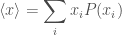
$\displaystyle \langle x \rangle = \sum_i x_i P(x_i)$ ,

where $\sum_i$ means sum over all values of $i$ (over all outcomes). The expectation value for rolling a die is

$\displaystyle \langle x \rangle = 1 \times P(1) + 2 \times P(2) + 3 \times P(3) + 4 \times P(4) + 5 \times P(5) + 6 \times P(6) = \frac{7}{2}$ .

The expectation value of a distribution is its average, the value you’d expect after many (infinite) repetitions. (Of course this is possible in reality—you’d certainly get RSI—but it is useful for keeping statisticians out of mischief).

For a continuous distribution, the expectation value is given by

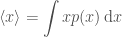
$\displaystyle \langle x \rangle = \int x p(x) \, \mathrm{d} x$ ,

where $p(x)$ is the probability density function.

You can use the expectation value to guide predictions for the outcome. You can never predict with complete accuracy (unless there is only one possible outcome), but you can use knowledge of the probabilities of the various outcomes the inform your predictions.

Imagine that after buying a large quantity of fudge, for entirely innocent reasons, the owner offers you the chance to play double-or-nothing—you’ll either pay double the bill or nothing, based on some random event—should you play? Obviously, this depends upon the probability of winning. Let’s say that the probability of winning is $p$ and find out how high it needs to be to be worthwhile. We can use the expectation value to calculate how much we should expect to pay, if this is less than the bill as it stands, it’s worth giving it a go, if the expectation value is larger than the original bill, we should expect to pay more (and so probably shouldn’t play). The expectation value is

$\displaystyle \langle x \rangle = 0 \times (1 - p) + 2 \times p = 2 p$ ,

where I’m working in terms of unified fudge currency, which, shockingly, is accepted in very few shops, but has the nice property that your fudge bill is always 1. Anyhow, if $\langle x \rangle$ is less than one, so if $p < 0.5$ , it’s worth playing. If we were tossing a (fair) coin, we’d expect to come out even, if we had to roll a six, we’d expect to pay more.

The expectation value is the equivalent of the mean. This is the average that people usually think of first. If you have a set of numeric results, you calculate the mean by adding up all or your results and dividing by the total number of results $N$ . Imagine each outcome $x_i$ occurs $n_i$ times, then the mean is

$\displaystyle \bar{x} = \sum_i x_i \frac{n_i}{N}$ .

We can estimate the probability of each outcome as $P(x_i) = n_i/N$ so that $\bar{x} = \langle x \rangle$ .

Median and mode

Aside from the mean there are two other commonly used averages, the median and the mode. These aren’t quite as commonly used, despite sounding friendlier. With a set of numeric results, the median is the middle result and the mode is the most common result. We can define equivalents for both when dealing with probability distributions.

To calculate the median we find the value where the total probability of being smaller (or bigger) than it is a half: $P(x < x_\mathrm{med}) = 0.5$ . This can be done by adding up probabilities until you get a half

$\displaystyle \sum_{x_i \, \leq \, x_\mathrm{med} } P(x_i) = 0.5$ .

For a continuous distribution this becomes

$\displaystyle \int_{x_\mathrm{low}}^{x_\mathrm{med}} p(x) \, \mathrm{d}x = 0.5$ ,

where $x_\mathrm{low}$ is the lower limit of the distribution. (That’s all the calculus out of the way now, so if you’re not a fan you can relax). The LD₅₀ lethal dose is a median. The median is effectively the middle of the distribution, the point at which you’re equally likely to be higher or lower.

The median is often used as it is not as sensitive as the mean to a few outlying results which are far from the typical values.

The mode is the value with the largest probability, the most probable outcome

$\displaystyle P(x_\mathrm{mode}) = \max P(x_i)$ .

For a continuous distribution, it is the point which maximises the probability density function

$\displaystyle p(x_\mathrm{mode}) = \max p(x)$ .

The modal value is the most probable outcome, the most likely result, the one to bet on if you only have one chance.

Education matters

Every so often, some official, usually an education minister, says something about wanting more than half of students to be above average. This results in much mocking, although seemingly little rise in the standards for education ministers. Having discussed averages ourselves, we can now see if it’s entirely fair to pick on these poor MPs.

The first line of defence, is that we should probably specify the distribution we’ve averaging. It may well be that they actually meant the average bear. It’s a sad truth that bears perform badly in formal education. Many blame the unfortunate stereotyping resulting from Winnie the Pooh. It might make sense to compare with performance in the past to see if standards are improving. We could imagine that taking the average from the 1400s would indeed show some improvement. For argument’s sake, let’s say that we are indeed talking about the average over this year’s students.

If the average we were talking about was the median, then it would be impossible for more (or fewer) than half of students to do better than average. In the case, it is entirely fair to mock the minister, and possibly to introduce them to the average bear. In this case, a mean bear.

If we were referring to the mode, then it is quite simple for more than half of the students to do better than this. To achieve this we just need a bottom-heavy distribution, a set of results where the most likely outcome is low, but most students do better than this. We might want to question an education system where the aim is to have a large number of students doing poorly though!

Finally, there is the mean; to use the mean, we first have to decide if we have a sensible if we are averaging a sensible quantity. For education performance this normally means exam results. Let’s sidestep the issue of if we want to reduce the output of the education system down to a single number, and consider the properties we want in order to take a sensible average. We want the results to be numeric (check); to be ordered, such that high is good and low is bad (or vice versa) so 42 is better than 41 but not as good as 43 and so on (check), and to be on a linear scale. The last criterion means that performance is directly proportional to the mark: a mark twice as big is twice as good. Most exams I’ve encountered are not like this, but I can imagine that it is possible to define a mark scheme this way. Let’s keep imagining, and assume things are sensible (and perhaps think about kittens and rainbows too… ).

We can construct a distribution where over half of students perform better than the mean. In this case we’d really need a long tail: a few students doing really very poorly. In this case, these few outliers are enough to skew the mean and make everyone else look better by comparison. This might be better than the modal case where we had a glut of students doing badly, as now we can have lots doing nicely. However, it also means that there are a few students who are totally failed by the system (perhaps growing up to become a minister for education), which is sad.

In summary, it is possible to have more than 50% of students performing above average, assuming that we are not using the median. It’s therefore unfair to heckle officials with claims of innumeracy. However, for these targets to be met requires lots of students to do badly. This seems like a poor goal. It’s probably better to try to aim for a more sensible distribution with about half of students performing above average, just like you’d expect.

An introduction to probability: Leaving nothing to chance

August 9, 2014October 25, 2014 / CPLB / Leave a comment

Probabilities and science

Understanding probabilities is important in science. Once you’ve done an experiment, you need to be able to extract from your data information about your theory. Only rarely do you get a simple yes or no: most of the time you have to work with probabilities to quantify your degree of certainty. I’ll (probably) be writing about probabilities in connection with my research, so I thought it would be useful to introduce some of the concepts.

I’ll be writing a series of posts, hopefully going through from the basics to the limits of my understanding. We’ll begin with introducing the concept of probability. There’s a little bit of calculus, but you can skip that without effecting the rest, just remember you can’t grow up to be big and strong if you don’t finish your calculus.

What is a probability?

A probability describes the degree of belief that you have in a proposition. We talk about probabilities quite intuitively: there are some angry-looking, dark clouds overhead and I’ve just lit the barbecue, so it’s probably going to rain; it’s more likely that United will win this year’s sportsball league than Rovers, or it’s more credible that Ted is exaggerating in his anecdote than he actually ate that much fudge…

We formalise the concept of a probability, so that it can be used in calculations, by assigning them numerical values (not by making them wear a bow-tie, although that is obviously cool). Conventionally, we use 0 for impossible, 1 for certain and the range in between for intermediate probabilities. For example, if we were tossing a coin, we might expect it to be heads half the time, hence the probability of heads is $P(\mathrm{head}) = 1/2$ , or if rolling a die, the probability of getting a six is $P(6) = 1/6$ .

For both the coin and the die we have a number of equally probable outcomes: two for the coin (heads and tails) and six for the die (1, 2, 3, 4, 5 and 6). This does not have to be the case: imagine picking a letter at random from a sample of English text. Some letters are more common than others—this is why different letters have different values in Scrabble and why hangman can be tricky. The most frequent letter is “e”, the probability of picking it is about 0.12, and the least frequent is “z”, the probability of picking that is just 0.0007.

Often we consider a parameter that has a continuous range, rather than discrete values (as in the previous examples). For example, I might be interested in the mass of a black hole, which can have any positive value. We then use a probability density function $p(x)$ such that the probability for the parameter lies in the range $a \leq x \leq b$ is given by the integral

$\displaystyle P(a \leq x \leq b) = \int_a^b p(x)\, \mathrm{d}x$ .

Performing an integral is just calculating the area under a curve, it can be thought of a the equivalent of adding up an infinite number of infinitely closely spaced slices. Returning to how much fudge Ted actually ate, we might to find the probability that he a mass of fudge $m$ that was larger than zero, but smaller than the fatal dose $M$ . If we a had probability density function $p(m)$ , we would calculate

$\displaystyle P(0 < m \leq M) = \int_0^{M} p(m)\, \mathrm{d}m$ .

The probability density is largest where the probability is greatest and smallest where the probability is smallest, as you’d expect. Calculating probabilities and probability distributions is, in general, a difficult problem, it’s actually what I spend a lot of my time doing. We’ll return to calculating probabilities later.

Combining probabilities

There are several recipes for combining probabilities to construct other probabilities, just like there are recipes to combine sugar and dairy to make fudge. Admittedly, probabilities are less delicious than fudge, but they are also less likely to give you cavities. If we have a set of of disjoint outcomes, we can work out the probability of that set by adding up the probabilities of the individual outcomes. For example, when rolling our die, the probability of getting an even number is

$\displaystyle P(\mathrm{even}) = P(2) + P(4) + P(6) = \frac{1}{6} +\frac{1}{6} +\frac{1}{6} = \frac{1}{2}$ .

(This is similar to what we’re doing when integrating up the probability density function for continuous distributions: there we’re adding up the probability that the variable $x$ is in each infinitesimal range $\mathrm{d}x$ ).

If we have two independent events, then the probability of both of them occurring is calculated by multiplying the two individual probabilities together. For example, we could consider the probability of rolling a six and the probability of Ted surviving eating the lethal dose of fudge, then

$\displaystyle P(\mathrm{6\: and\: survive}) = P(6) \times P(\mathrm{survive})$ .

The most commonly quoted quantity for a lethal dose is the median lethal dose or LD₅₀, which is the dose that kills half the population, so we can take the probability of surviving to be 0.5. Thus,

$\displaystyle P(\mathrm{6\: and\: survive}) = P(6) \times P(\mathrm{survive}) = \frac{1}{12}$ .

Events are independent if they don’t influence each other. Rolling a six shouldn’t influence Ted’s medical condition, and Ted’s survival shouldn’t influence the roll of a die, so these events are independent.

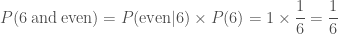
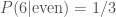
Things are more interesting when events are not independent. We then have to deal with conditional probabilities: the conditional probability $P(\mathrm{A}|\mathrm{B})$ is the probability of $\mathrm{A}$ given that $B$ is true. For example, if I told you that I rolled an even number, the probability of me having rolled a six is $P(6|\mathrm{even}) = 1/3$ . If I told you that I have rolled a six, then the probability of me having rolled an even number is $P(\mathrm{even}|6) = 1$ —it’s a dead cert, so bet all your fudge on that! When combining probabilities from dependent events, we chain probabilities together in a logical chain. The probability of rolling a six and an even number is the probability of rolling an even number multiplied by the probability of rolling a six given that I rolled an even number

$\displaystyle P(\mathrm{6\: and\: even}) = P(6|\mathrm{even}) \times P(\mathrm{even})= \frac{1}{3} \times \frac{1}{2} = \frac{1}{6}$ ,

or equivalently the probability of rolling six multplied by the probability of rolling an even number given that I rolled a six

$\displaystyle P(\mathrm{6\: and\: even}) = P(\mathrm{even} | 6) \times P(6) = 1 \times \frac{1}{6} = \frac{1}{6}$ .

Reassuringly, we do get the same answer. This is a bit of a silly example, as we know that if we’ve rolled a six we have rolled an even number, so all we are doing if calculating the probability of rolling a six.

We can use conditional probabilities for independent events: this is really easy as the conditional probability is just the straight probability. The probability of Ted surviving his surfeit of fudge given that I rolled a six is just the probability of him surviving, $P(\mathrm{survive}|6) = P(\mathrm{survive})$ .

Let’s try a more complicated example, let’s imagine that Ted is playing fudge roulette. This is like Russian roulette, except you roll a die and if it comes up six, then you have to eat the lethal dose of fudge. His survival probability now depends on the roll of the die. We want to calculate the probability that Ted will live to tomorrow. If Ted doesn’t roll a six, we’ll assume that he has a 100% survive rate (based on that one anecdote where he claims to have created a philosopher’s stone by soaking duct tape in holy water), this isn’t quite right, but is good enough. The probability of Ted surviving given he didn’t roll a six is

$\displaystyle P(\mathrm{not\: 6\: and\: survive}) = P(\mathrm{survive} | \mathrm{not\: 6}) \times P(\mathrm{not\: 6}) = 1 \times \frac{5}{6} = \frac{5}{6}$ .

The probability of Ted rolling a six (and eating the fudge) and then surviving is

$\displaystyle P(\mathrm{6\: and\: survive}) = P(\mathrm{survive} | \mathrm{6}) \times P(\mathrm{6}) = \frac{1}{2} \times \frac{1}{6} = \frac{1}{12}$ .

We have two disjoint outcomes (rolling a six and survivng, and not rolling a six and surving), so the total probability of surviving is given by the sum

$\displaystyle P(\mathrm{survive}) =P(\mathrm{not\: 6\: and\: survive}) +P(\mathrm{6\: and\: survive}) = \frac{5}{6} +\frac{1}{12} =\frac{11}{12}$ .

It seems likely that he’ll make it, although fudge roulette is still a dangerous game!

There’s actually an easier way of calculating the probability that Ted survives. There are only two possible outcomes: Ted survives or he doesn’t. Since one of these must happen, their probabilities must add to one: the survive probability is

$P(\mathrm{survive}) = 1 - P(\mathrm{not\: survive})$ .

We’ve already seen this, as we’ve used the probability of not rolling a six is $P(\mathrm{not\: 6}) = 1 - P(6) = 5/6$ . The probability of not surviving is much easier to work out as there’s only one way that can happen: rolling a six and then overdosing on fudge. The probability is

$\displaystyle P(\mathrm{not\: surviving}) = P(\mathrm{fudge\: overdose}|6) \times P(6) = \frac{1}{2} \times \frac{1}{6} = \frac{1}{12}$ ,

and so the survival probability is $P(\mathrm{survive}) = 1 - 1/12 = 11/12$ , exactly as before, but in fewer steps.

In a future post we’ll try working out the probability that Ted did eat a lethal dose of fudge given that he is alive to tell the anecdote. This is known as an inverse problem, and is similar to what scientists do all the time. We do experiments and get data, then we need to work out the probability of our theory (that Ted ate the fudge) being correct given the data (that he’s still alive).

Interpreting probabilities

We have now discussed what a probability is and how we can combine them. We should now think about how to interpret them. It’s easy enough to understand that a probability of 0.05 means that we expect something should happen on average once in 20 times, and that it is more probable than something with a probability of 0.01, but less likely than something with a probability of 0.10. However, we are not good at having an intuitive understanding of probabilities.

Consider the case that a scientist announces a result with 95% confidence. That sounds pretty good. Think how surprised you would be (assuming that their statistics are all correct) that the result was wrong. I feel like I would be pretty surprised. Now consider rolling tow dice, how surprised would you be if you rolled two sixes? The probability of the result being wrong is $1 - 0.95 = 0.05$ , or one in twenty. The probability of rolling two sixes is $1/6 \times 1/6 = 1/36$ or about one in forty. Hence, you should be almost twice as surprised by rolling double six as for a 95% confidence-level result being incorrect.

When dealing with probabilities, I find it useful to make a comparison to something familiar. While Ted is more likely than not to survive fudge roulette, there is a one is twelve chance of dying. That’s three times as likely as rolling a double six, or equally probable as rolling a six and getting heads. That’s riskier than I’d like, so I’m going to stick to consuming fudge in moderation.