GW200115 and GW200105 are the first gravitational-wave candidates announced from the second half of LIGO and Virgo’s third observing run (O3b). They may be our first ever observations of neutron star–black hole binaries [bonus note]. These mixed binaries of one neutron star and one black hole have long proved elusive, but we are now on our way to revealing their secrets.

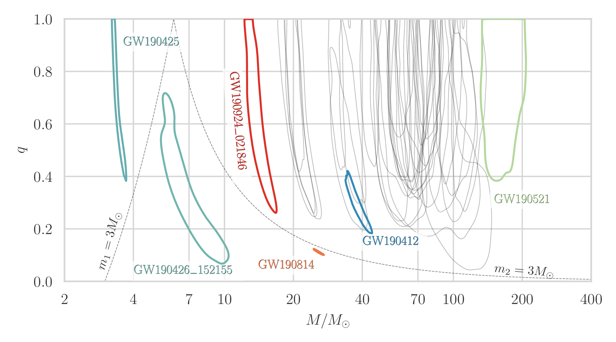
The population of compact objects (black holes and neutron stars) observed with gravitational waves and with electromagnetic astronomy, including a few that are uncertain. The sources for GW200115 (left) and GW200105 (right) are highlighted. Source: Northwestern
The first gravitational-wave signal ever detected, GW150914, came from a binary black hole system: two black holes that inspiralled together to form a bigger black hole. (I hope you are all imagining a bloopy chirp to accompany this). We had never before observed a binary black hole system. However, binary black holes have proved to be the most common source of gravitational waves, and we are now starting to understand their properties. We found our next type of gravitational-wave source with GW170817, which came from a binary neutron star system (two neutron stars that orbited each other). Before we had gravitational-wave astronomy, we knew this type of binary existed as we had observed pulsars in binaries thanks to radio astronomy. Yet, our second binary neutron star observation, GW190425, still showed that we didn’t know everything about their properties. After finding binary black holes and binary neutron stars, what about a mixed neutron star–black hole binary? These should exist, but finding evidence for them has proved difficult.
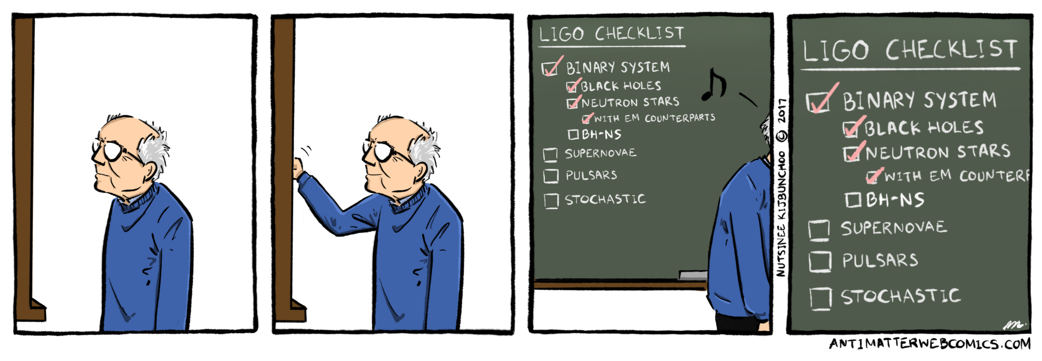
Time to tick neutron star–black hole binaries off the checklist. Part of a comic by Nutsinee Kijbunchoo drawn following the discovery of GW170817 showing Rai Weiss rather happy with his work. [Update]
Previous candidates
The first hints of neutron star–black hole binaries came in the first half of LIGO and Virgo’s third observing run (O3a, yes we are the best at thinking up names). The gravitational-wave candidate GW190426_152155 (the best at names) looks like it could have come from a neutron star–black hole binary. However, this is a quiet signal, so we are not sure whether it is real or a false alarm.
Our detection pipelines search the data from the detectors looking for signals. Our searches designed to specifically look for signals from binaries match the data against templates of what the signals should look like. From this comparison, they consider two pieces of information: how loud a signal is (its signal-to-noise ratio), and how consistent the signal is with the template. These are combined into a ranking statistic, and by comparing the ranking statistic with values produced by a background of noise, we can compute a false alarm rate of how often something at least this signal-like would happen in random noise. For GW190426_152155, this is 
The false alarm rate is not the end of the story though: we need to consider the true alarm rate: how often we expect to detect such a signal. If something is an everyday occurrence, you don’t need much evidence to convince yourself it’s real. Consider the quality of a photo you would need to convince yourself there was a horse walking around outside, and the quality needed to convince yourself there is a unicorn. For gravitational waves, a false alarm rate of
Estimated total mass 
The next potential candidate was GW190814. This is a super clear detection. However, the nature of the source is more mysterious. The primary (the more massive object in the binary) is definitely a black hole, but the secondary, at around 

Discovery
Observations in O3b changed everything. Within the space of ten days in January 2020 [bonus note], we collected two neutron star–black hole candidates: GW200105_162426 (GW200105 for short) and GW200115_042309 (GW200115).
GW200115 is a clear detection. All three detectors were observing at the time, and we get a good signal in both LIGO Livingston and LIGO Hanford (Virgo, being less sensitive currently, has less informative data). From these observations, our search algorithm GstLAL estimates a false alarm rate of 

GW200105 is more difficult. LIGO Hanford was offline at the time, so we only have LIGO Livingston and Virgo. In Livingston data we can see a beautiful chirp, but in Virgo the signal is too quiet for the detection algorithms to use. This is like the case for GW190425, we must try to establish the significance using a single detector.

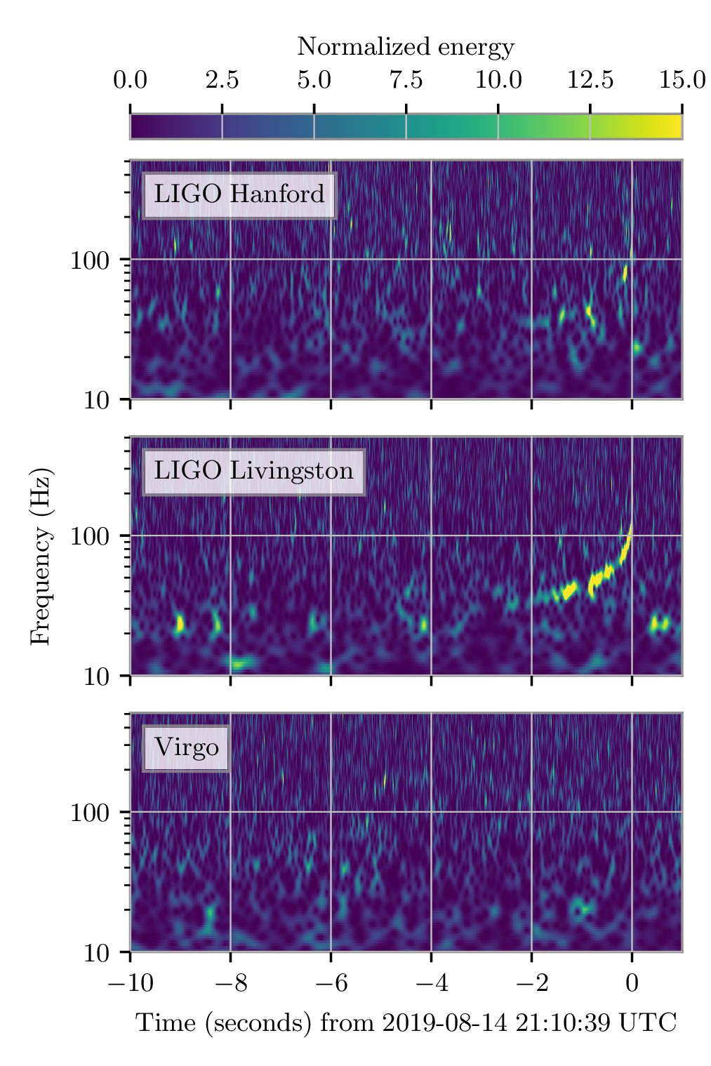
Time–frequency plots for GW200105 (left) and GW200115 (right) as measured by LIGO Hanford, LIGO Livingston and Virgo. LIGO Hanford was not observing at the time of GW200105. The chirp of a binary coalescence is clearest in Livingston for GW200105; these are usually hard to see for these types of signals. The Livingston data for GW200105 is shown after glitch subtraction, and the Livingston data for GW200115 shows light-scattering glitches at low frequencies. Figure 1 of the NSBH Discovery Paper.
When we have multiple detectors, we can ask how often we would expect to see the same signal at compatible times in multiple detectors. It is much less likely that multiple detectors would have the same random bit of noise in one detector and at the same time in another. We can estimate how often this would happen, for example, by comparing data from the detectors at different times. Considering many different time offsets, we can build up statistics for tens of thousands of years, even though we have only been observing for a few months (the upper limit on the false alarm rate quoted for GW200115 is because it stands out after we have exhausted all these times slides). When we have a single detector, we can’t do this.
GW200105 stands out from anything we have seen in the data we’ve analysed. We could therefore assign a false alarm rate of one per observing time. However, that doesn’t quite encode everything we know. We expect louder noise artifacts to be rarer than quieter ones. An outlier with signal-to-noise ratio of 12 should be rarer than one with signal-to-noise ratio of 11 (and GW200105 is over 13), and hence we can use this knowledge to try to extrapolate a false alarm rate.

Detection statistics for GW200105, GW200115 and GW190426_152155, showing they compare to background data. The plot shows the signal-to-noise 

Currently, only GstLAL can calculate single-detector false alarm rates. PyCBC and MBTA both identify the same feature in the data, but cannot assign a significance to this. Using GstLAL’s extrapolation, which is chosen to be conservative (not as conservative as one per observing time, but a better representation of the data), we calculate a false alarm rate of 
It is very tempting to look at GW200105‘s clear chirp and convince yourself it must be real. However, our detection algorithms are more sensitive than our eyes and more reliable. They are carefully tested, and build up their statistics analysing large chunks of data. Hence, we should acknowledge that the difficulty in assigning a false alarm rate is an intrinsic difficulty when you only have so much data. Even the best signal can only end up with a modest false alarm rate. It’s kind of like winning the lottery on your third go if you don’t know how the lottery works: you can estimate that the probability of winning is about 1/3, even if you suspect it should be much smaller. The results computed for this paper only use a fraction of O3b, so we could be able to do a little better in the future.
Sources
Let us assume both signals are real, where do they come from? Do we at last have our undisputable neutron star–black hole binaries?
We infer [bonus note] that GW200115 comes from a binary with component masses 


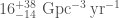
For GW200105, we infer that the primary has mass 


Estimated masses for the binary primary and secondary masses 

The masses for GW200115 overlap nicely with those inferred for GW190426_152155 

The masses align nicely with expectations for neutron star–black hole binaries, so there are no surprises there. Ideally, we would confirm that we have seen neutron stars by measuring the tidal distortion of the neutron star [bonus note]. Unfortunately, these effects get harder to measure when the asymmetry in masses gets more significant, and we can’t pick anything out of the data. However, we did compare the secondary masses to various expectations for the maximum neutron star mass, and find that there’s over a 93% probability that the secondaries are safely below this. In conclusion, I think we have a good case for having completed our set of binaries and found neutron star–black hole binaries.
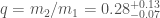
Estimated orientation and magnitude of the two component spins for GW200105 (left) and GW200115 (right). The distribution for the more massive primary component is on the left, and for the lighter secondary component on the right. The probability is binned into areas which have uniform prior probabilities, so if we had learnt nothing, the plot would be uniform. The maximum spin magnitude of 1 is appropriate for black holes. The solid line shows the 90% credible region using the high spin prior (which is used for the rest of the plot) and the dashed line shows the 90% contour for the low-spin prior. Figure 6 of the NSBH Discovery Paper.
The spins are more interesting. Spins range from zero for non-spinning, to one for a maximally spinning black hole. As a consequence of the large mass asymmetry, we measure the spin of the black holes better than for the neutron stars. For GW200105, we can constrain the spin magnitude to be 

For GW200115, the primary spin is also consistent with zero. However, there is also support for larger spins, and intriguingly, spin misaligned (or even antialigned as there’s little evidence of spin components in the orbital plane) with the orbital angular momentum. It is often convenient to work with the effective inspiral spin, which is a mass-weighted combination of the two spins projected along the direction of the orbital momentum. A positive value indicates the spins are overall aligned with the orbital angular momentum, while a negative value indicates the spins are overall misaligned. For GW200105, we find 


Generally aligned spins are expected for binaries formed from two binary stars that lived their lives together. The stars would have formed from the same cloud of gas, so you would expect the stars to start out rotating the same way. Tides and mass transfer between the stars should also help to align spins. Supernova explosions could tilt the spins, but it’s hard to get a complete reversal without disrupting the binary. This did happen for the double pulsar, so it’s not impossible, but overall you would expect it to be rare. However, for binaries formed dynamically, the spins would be randomly aligned.
Does the spin for GW200115 thus point to a dynamical origin? That would be unexpected, as isolated evolution generally predicts higher rates of forming neutron star–black hole binaries than dynamical channels. Dynamical channels tend to prefer making more massive binaries. The spin is perfectly consistent with being small and aligned, so perhaps that is the correct answer, and there’s nothing unexpected to see.
Estimated primary mass 

Since the spin is correlated with the mass, if we impose that GW200115‘s primary spin is small and aligned, we also find that the primary mass is towards the upper end of its range. This would keep it safely out of the proposed range of the lower mass gap. I’m not sure if that is of any physical relevance (as I’m not sure if I believe there is a gap), but it is potentially worth keeping in mind if you want to model the progenitor (you need to fit mass and spin together).
I look forward to lots of studies looking at how to form these systems.
Rates
Now we have confirmation that neutron star–black hole binaries exist, how many do we think there are out there? To go from our detections to a merger rate density, we need to assume something about the population of neutron star–black hole binaries (we need to know about the systems that we could have observed but didn’t). This is rather tricky, as neutron star–black hole binaries could potentially have a diverse range of properties, and we can’t be sure of this distribution with only a couple of observations. Therefore, we’ve tried a few different things.
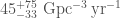
First, we considered what are the rates of binaries that match the inferred properties of the two sources. We infer that the rate of GW200115-like binaries is 

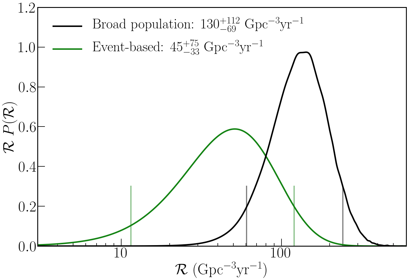
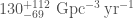
Probability distribution for the neutron star–black hole binary merger rate density. The green curve shows the event-based rate assuming all neutron star–black hole binaries are like GW200105 or GW200115. The black line assumes a broader population that also includes GW190814 and higher mass black holes. The vertical lines mark the 90% credible interval. Figure 9 of the NSBH Discovery Paper.
The second approach is to take a much more agnostic approach, and consider all output from our detection pipelines over a plausible mass range. The population here is defined more for convenience than anything else. We picked search triggers (down to a signal-to-noise ratio) corresponding to binaries with a primary mass between 


I don’t think these will rule out any models, but they give the ballpark to aim for. As we find more neutron star–black hole candidates, these rates should evolve as our uncertainties will shrink, and we get a better understanding of the source population.
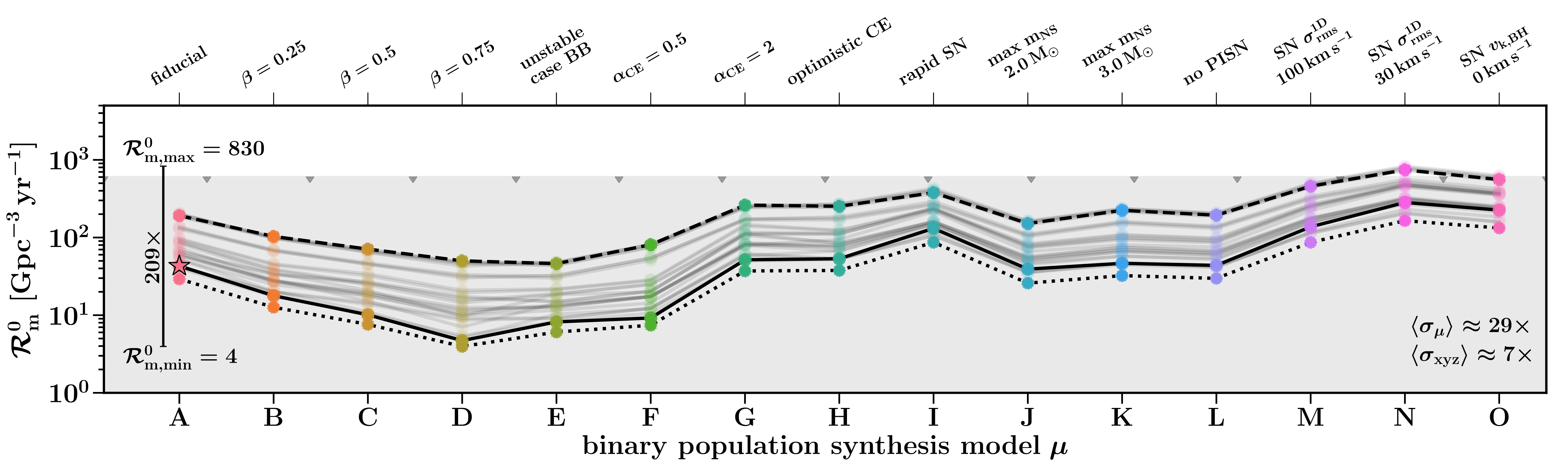
Predictions for the neutron star–black hole binary merger rate density as modelled by the COMPAS population synthesis code. The different models illustrate variations in the input physics, highlighting the range of predictions for isolated binary evolution. Other channels could potentially form neutron star–black hole binaries too. Figure 9 of Broekgaarden et al. (2021).
Summary
We have finally found our neutron star–black hole binaries. They’re pretty neat. These are the first discoveries from O3b. They will not be the last.
Title: Observation of gravitational waves from two neutron star–black hole coalescences
Journal: Astrophysical Journal Letters; 915(1):L5(25)
arXiv: 2106.15163 [astro-ph.HE]
Science summary: A new source of gravitational waves: Neutron star–black hole binaries
Data release: GW200105; GW200115
GW200105 Rating: 🐦🍨🥇😮
GW200115 Rating: 🐭🍨😮🙃🏆
Bonus notes
Cookies
I like to think of neutron star–black hole binaries as the mirror counterparts of fluffernutter cookies. Black holes are black and super dense, completely unlike marshmallows. Neutron stars are made of something mysterious that we don’t know the properties of, but we think all neutron stars are made of the same type of stuff™, whereas peanut butter is made of well known ingredients, but has both smooth and crunchy equations of state. Despite the difference in ingredients, for both, when we mix the two types we get something delicious.
Even years
Previously, all our LIGO–Virgo discoveries came during odd-numbered years, so I was kind of hoping for a quiet 2020. This didn’t work out.
Waveform models
One of the most difficult things with inferring the properties of neutron star–black hole binaries is the waveform models that we use. We need accurate models to compare with the data to get good estimates of the parameters. Unfortunately, we don’t have models that include all the physics we want (spin precession, higher-order multipole moments, and the effects of the neutron star stuff™). From our tests, it seems like spin precession and higher-order multipole moments are more important. The latter is certainly important for asymmetric binaries. Therefore, for our main results, we use binary black hole waveforms that include spin precession and higher-order multipole moments (but no neutron star stuff™ effects). These models should be a pretty good representation of the overall physics (especially if the neutron tar gets swallowed whole). However, they may not give the best estimate of the final black hole mass. In the paper, we used the neutron star–black hole waveforms that include neutron star stuff™ effects but not spin precession and higher-order multipole moments, but I think it’s a bit confusing to mix the two results here, so I’ll skip over final masses and spins.
GW190426_152155’s properties
While GW190426_152155 agrees nicely with GW200115‘s masses, its other properties are somewhat different. Its effective inspiral spin is 


Electromagnetic observations
An electromagnetic counterpart, as was found for GW170817, would confirm the presence of stuff™, and that we didn’t just have two black holes. However, with these mass black holes, we would expect the neutron stars to be pretty much swallowed whole (like me consuming a fluffernutter cookie) with nothing to see [bonus bonus note]. So far nothing has been reported, which is about as surprising as failing to find a needle in a haystack, when there is no needle.
Ejecta
We estimate that the amount of neutron star stuff ejected during the merger is less than 


 . All contours are for 90% probabilities. Figure 2 of the
  solar masses (quoting the 90% range for parameters), and the other
  solar masses. This is remarkable for two reasons: first, the lower mass object is right in the range where we might hit the maximum mass of a neutron star, and second, this is the most asymmetric masses from any of our gravitational wave sources.
 . We show results several different waveform models (which include spin precession and higher order multiple moments). The two-dimensional shows the 90% probability contour. The one-dimensional plot shows individual masses; the dotted lines mark 90% bounds away from equal mass. Estimates for the maximum neutron star mass are shown for comparison with the mass of the lighter component
  M&Ms (plain; for peanut butter it would be different, and of course, more delicious) into the volume of just
  M&Ms (ignoring the fact that you can’t perfectly pack them)! Neutron stars are about
  times more dense than M&Ms. As you make neutron stars heavier, their gravity gets stronger until at some point the strange stuff™ they are made of can’t take
  and the tidal deformability
  .
.
 . The mass ratio changes a few things about the gravitational wave signal. When you have unequal masses, it is possible to observe
  . We again spot the next harmonic in GW190814, this time it is even more clear. Modelling gravitational waves from systems with mass ratios of
  is tricky, it is important to include the higher order multipole moments in order to get good estimates of the source parameters.
 . This is our best ever measurement of black hole spin!
 . Harder to measure is the spin in the orbital plane. This controls the amount of spin precession (wobbling in the spin orientation as the orbital angular momentum is not aligned with the total angular momentum), and is characterised by the effective precession spin parameter. For GW190814, we find
  , which is our tightest measurement. It might seem odd that we get our best measurement of in-plane spin in the case when there is no precession. However, this is because if there were precession, we would clearly measure it. Since there is no support for precession in the data, we know that it isn’t there, and hence that the amount of in-plane spin is small.
 . From GW190814 alone, we get
  (quoting numbers with our usual median and symmetric 90% interval convention; if you like mode and narrowest 68% region, it’s
  ). If we combine with results for GW170817, we get
  (or
(or  ) [
) [ . If you think you know how GW190814 formed, you’ll need to make sure to get a compatible rate estimate.
 is the orbital separation,
  is the orbital inclination,
  is the time since the stars started their life on the main sequence. The letters on the right indicate the evolution phase: ZAMS is zero-age main sequence, MS is main sequence (burning hydrogen), CHeB is core helium burning (once the hydrogen has been used up), and BH and NS mean black hole and neutron star. At low metallicities
  (when stars have few elements heavier than hydrogen and helium), the two channels are about as common, as metallicity increases Channel A becomes more common. Figure 6 of
  . The luminosity distance is a measure which incorporates the effects of the signal travelling through an expanding Universe, so it’s not quite the same as the actual distance between us and the source. Given the uncertainties on the luminosity distance, it would have taken the signal somewhere between 600 million and 850 million years to reach us. It therefore set out during the
  calories. That seems like a lot of energy, but it’s less than
  of the energy emitted as gravitational waves for GW190814.
 (mode and narrowest 68% region) using GW190814. Adding in GW170814 they get
  as a gravitational-wave-only measurement, and including GW170817 and its electromagnetic counterpart gives
  .
. .
.
 is the merger rate, and
  is the surveyed time–volume (you expect more detections if your detectors are more sensitive, so that they can find signals from further away, or if you leave them on for longer). We can estimate
  . We use a uniform prior, for consistency with what we’ve done in the past.
 confidence level limit on the rate is
 ,
,
 , the equivalent results is
![\displaystyle R_c = \frac{\left[\mathrm{erf}^{-1}(c)\right]^2}{\langle VT \rangle}](https://s0.wp.com/latex.php?latex=%5Cdisplaystyle+R_c+%3D+%5Cfrac%7B%5Cleft%5B%5Cmathrm%7Berf%7D%5E%7B-1%7D%28c%29%5Cright%5D%5E2%7D%7B%5Clangle+VT+%5Crangle%7D&bg=ffffff&fg=444444&s=0&c=20201002) ,
, , so results would be the same to within a factor of 2, but the results with the uniform prior are more conservative.
 for isotropic spins up to 0.05, and
  if you allow the spins up to 0.4.
 to
to  for a 1.4 solar mass neutron star and a black hole between 30 and 5 solar masses and a range of different spins (Table II of the
 and if they all come from neutron star–black hole mergers the angle needs to be bigger than
  .
.
 , and define an effective distance
  defined so that
  where
where  is the analysed amount of time. The plot below show our limits on rate and effective distance for our different injections.
 indicates the spin aligned with the orbital angular momentum. Figure 2 of the
