The Universe is full of awesome things. These posts will hopefully explain a few of these while pointing out some mysteries still to be solved. There’s probably a bias towards black holes because they’re especially awesome.
GW200115 and GW200105 are the first gravitational-wave candidates announced from the second half of LIGO and Virgo’s third observing run (O3b). They may be our first ever observations of neutron star–black hole binaries [bonus note]. These mixed binaries of one neutron star and one black hole have long proved elusive, but we are now on our way to revealing their secrets.
The population of compact objects (black holes and neutron stars) observed with gravitational waves and with electromagnetic astronomy, including a few that are uncertain. The sources for GW200115 (left) and GW200105 (right) are highlighted. Source: Northwestern
The first gravitational-wave signal ever detected, GW150914, came from a binary black hole system: two black holes that inspiralled together to form a bigger black hole. (I hope you are all imagining a bloopy chirp to accompany this). We had never before observed a binary black hole system. However, binary black holes have proved to be the most common source of gravitational waves, and we are now starting to understand their properties. We found our next type of gravitational-wave source with GW170817, which came from a binary neutron star system (two neutron stars that orbited each other). Before we had gravitational-wave astronomy, we knew this type of binary existed as we had observed pulsars in binaries thanks to radio astronomy. Yet, our second binary neutron star observation, GW190425, still showed that we didn’t know everything about their properties. After finding binary black holes and binary neutron stars, what about a mixed neutron star–black hole binary? These should exist, but finding evidence for them has proved difficult.
Time to tick neutron star–black hole binaries off the checklist. Part of a comic by Nutsinee Kijbunchoo drawn following the discovery of GW170817 showing Rai Weiss rather happy with his work. [Update]
Previous candidates
The first hints of neutron star–black hole binaries came in the first half of LIGO and Virgo’s third observing run (O3a, yes we are the best at thinking up names). The gravitational-wave candidate GW190426_152155 (the best at names) looks like it could have come from a neutron star–black hole binary. However, this is a quiet signal, so we are not sure whether it is real or a false alarm.
Our detection pipelines search the data from the detectors looking for signals. Our searches designed to specifically look for signals from binaries match the data against templates of what the signals should look like. From this comparison, they consider two pieces of information: how loud a signal is (its signal-to-noise ratio), and how consistent the signal is with the template. These are combined into a ranking statistic, and by comparing the ranking statistic with values produced by a background of noise, we can compute a false alarm rate of how often something at least this signal-like would happen in random noise. For GW190426_152155, this is , which isn’t too great.
The false alarm rate is not the end of the story though: we need to consider the true alarm rate: how often we expect to detect such a signal. If something is an everyday occurrence, you don’t need much evidence to convince yourself it’s real. Consider the quality of a photo you would need to convince yourself there was a horse walking around outside, and the quality needed to convince yourself there is a unicorn. For gravitational waves, a false alarm rate of would be enough to give you a fair (but not necessarily conclusive) probability of the signal being real if the source were a binary black hole, as we know they are pretty common. We don’t yet know how common gravitational waves from neutron star–black hole binaries are, but the fact that we are lacking good examples indicates that they are at least somewhat rare. Therefore, with the balance of probability, it seems plausible that GW190426_152155 is noise, and the hunt needs to continue.
Estimated total mass and mass ratio $q = m_2/m_1 \leq 1$ of the binary sources for the candidates in O3a. The contours mark the 90% credible regions. The dashed lines mark a robust upper limit on the maximum neutron star mass. Figure 6 of the GWTC-2 Paper.
The next potential candidate was GW190814. This is a super clear detection. However, the nature of the source is more mysterious. The primary (the more massive object in the binary) is definitely a black hole, but the secondary, at around (where is a solar mass) is either potentially too large to be a neutron star. We’re not entirely sure of the maximum mass a neutron star can be before collapsing. Hence, we’re not quite sure if we have a massive neutron star, or a really small black hole. I think the black hole is more likely. The curious nature of GW190814’s source means we are still missing an unambiguous neutron star–black hole.
Discovery
Observations in O3b changed everything. Within the space of ten days in January 2020 [bonus note], we collected two neutron star–black hole candidates: GW200105_162426 (GW200105 for short) and GW200115_042309 (GW200115).
GW200115 is a clear detection. All three detectors were observing at the time, and we get a good signal in both LIGO Livingston and LIGO Hanford (Virgo, being less sensitive currently, has less informative data). From these observations, our search algorithm GstLAL estimates a false alarm rate of , PyCBC estimates , and MBTA (being used for the first time for final search results) estimates . All of the search algorithms agree that this is a significant detection.
GW200105 is more difficult. LIGO Hanford was offline at the time, so we only have LIGO Livingston and Virgo. In Livingston data we can see a beautiful chirp, but in Virgo the signal is too quiet for the detection algorithms to use. This is like the case for GW190425, we must try to establish the significance using a single detector.
Time–frequency plots for GW200105 (left) and GW200115 (right) as measured by LIGO Hanford, LIGO Livingston and Virgo. LIGO Hanford was not observing at the time of GW200105. The chirp of a binary coalescence is clearest in Livingston for GW200105; these are usually hard to see for these types of signals. The Livingston data for GW200105 is shown after glitch subtraction, and the Livingston data for GW200115 shows light-scattering glitches at low frequencies. Figure 1 of the NSBH Discovery Paper.
When we have multiple detectors, we can ask how often we would expect to see the same signal at compatible times in multiple detectors. It is much less likely that multiple detectors would have the same random bit of noise in one detector and at the same time in another. We can estimate how often this would happen, for example, by comparing data from the detectors at different times. Considering many different time offsets, we can build up statistics for tens of thousands of years, even though we have only been observing for a few months (the upper limit on the false alarm rate quoted for GW200115 is because it stands out after we have exhausted all these times slides). When we have a single detector, we can’t do this.
GW200105 stands out from anything we have seen in the data we’ve analysed. We could therefore assign a false alarm rate of one per observing time. However, that doesn’t quite encode everything we know. We expect louder noise artifacts to be rarer than quieter ones. An outlier with signal-to-noise ratio of 12 should be rarer than one with signal-to-noise ratio of 11 (and GW200105 is over 13), and hence we can use this knowledge to try to extrapolate a false alarm rate.
Detection statistics for GW200105, GW200115 and GW190426_152155, showing they compare to background data. The plot shows the signal-to-noise ratio and signal-consistency statistic from the GstLAL algorithm. The coloured density plot shows the distribution of background triggers. LHO indicates a trigger from LIGO Hanford, and LLO indicates a trigger from LIGO Livingston. GW200105 is distinct from anything else seen in O3. However, GW200105 is calculated less significant than GW200115 as it only has a trigger from a single detector. Figure 3 of the NSBH Discovery Paper.
Currently, only GstLAL can calculate single-detector false alarm rates. PyCBC and MBTA both identify the same feature in the data, but cannot assign a significance to this. Using GstLAL’s extrapolation, which is chosen to be conservative (not as conservative as one per observing time, but a better representation of the data), we calculate a false alarm rate of . This is good enough to be interesting, and better than for GW190426_152155, but not enough to be absolutely conclusive. I think we may see some active development of estimating single-detector false alarm rates (or lowering the threshold for Virgo data to be used) in the future to try to address these difficulties.
It is very tempting to look at GW200105‘s clear chirp and convince yourself it must be real. However, our detection algorithms are more sensitive than our eyes and more reliable. They are carefully tested, and build up their statistics analysing large chunks of data. Hence, we should acknowledge that the difficulty in assigning a false alarm rate is an intrinsic difficulty when you only have so much data. Even the best signal can only end up with a modest false alarm rate. It’s kind of like winning the lottery on your third go if you don’t know how the lottery works: you can estimate that the probability of winning is about 1/3, even if you suspect it should be much smaller. The results computed for this paper only use a fraction of O3b, so we could be able to do a little better in the future.
Sources
Let us assume both signals are real, where do they come from? Do we at last have our undisputable neutron star–black hole binaries?
We infer [bonus note] that GW200115 comes from a binary with component masses and (or and if we restrict the secondary’s spin to ). The primary here looks to be a black hole. It is one of the smallest we have seen. The uncertainties on the measurement potentially take it into the hypothesised lower mass gap between neutron stars and black holes suggested from X-ray observations (and somewhat questioned by GW190814); however, there is a 70% chance that the mass is , so it is pretty consistent with the population of black holes we’ve seen in X-ray binaries. The secondary is perfectly in the neutron star range. Hence, this looks like a great neutron star–black hole binary candidate.
For GW200105, we infer that the primary has mass and secondary has mass (or and with low secondary spin). The primary is a nice black hole, the secondary is a nice plump neutron star. It is towards the more massive end of the distribution we have seen with radio observations, but it is consistent with past observations. Unlike for GW190814, we do not have any trouble explaining such as mass given what we know about the stiffness of neutron star stuff™. This is another good neutron star–black hole binary candidate.
Estimated masses for the binary primary and secondary masses and for neutron star–black hole binary candidates. The two-dimensional plot shows the 90% probability contour. For GW200105 and GW200115 we show results for two different spin priors for the secondary. The one-dimensional plot shows individual masses; the vertical lines mark 90% bounds away from equal mass. Estimates for the maximum neutron star mass (based upon Galactic neutron stars and studies of the equation of state) are shown for comparison with the mass of the secondary. Figure 4 of the NSBH Discovery Paper.
The masses for GW200115 overlap nicely with those inferred for GW190426_152155 and [bonus note]. The uncertainties for GW190426_152155 are larger, on account of it being quieter. Perhaps this could indicate this is fairly typical for neutron star–black hole binaries (and we might need to revise that true alarm rate)? It’s still too early to say, but I very much look forward to finding out!
The masses align nicely with expectations for neutron star–black hole binaries, so there are no surprises there. Ideally, we would confirm that we have seen neutron stars by measuring the tidal distortion of the neutron star [bonus note]. Unfortunately, these effects get harder to measure when the asymmetry in masses gets more significant, and we can’t pick anything out of the data. However, we did compare the secondary masses to various expectations for the maximum neutron star mass, and find that there’s over a 93% probability that the secondaries are safely below this. In conclusion, I think we have a good case for having completed our set of binaries and found neutron star–black hole binaries.
Estimated orientation and magnitude of the two component spins for GW200105 (left) and GW200115 (right). The distribution for the more massive primary component is on the left, and for the lighter secondary component on the right. The probability is binned into areas which have uniform prior probabilities, so if we had learnt nothing, the plot would be uniform. The maximum spin magnitude of 1 is appropriate for black holes. The solid line shows the 90% credible region using the high spin prior (which is used for the rest of the plot) and the dashed line shows the 90% contour for the low-spin prior. Figure 6 of the NSBH Discovery Paper.
The spins are more interesting. Spins range from zero for non-spinning, to one for a maximally spinning black hole. As a consequence of the large mass asymmetry, we measure the spin of the black holes better than for the neutron stars. For GW200105, we can constrain the spin magnitude to be at 90% probability (or with the low neutron star spin prior). This matches what we have seen for a lot of our black holes (as for GW190814‘s primary, but probably not for GW190412‘s primary), that their spins are small and nicely consistent with being zero.
For GW200115, the primary spin is also consistent with zero. However, there is also support for larger spins, and intriguingly, spin misaligned (or even antialigned as there’s little evidence of spin components in the orbital plane) with the orbital angular momentum. It is often convenient to work with the effective inspiral spin, which is a mass-weighted combination of the two spins projected along the direction of the orbital momentum. A positive value indicates the spins are overall aligned with the orbital angular momentum, while a negative value indicates the spins are overall misaligned. For GW200105, we find (or with low neutron star spin). This is consistent with zero, and what you would expect if spins were small, or if there were no preferred alignment. For GW200115 however, we find ( with low neutron star spin). This is still consistent with positive or zero values, but prefers negative values.
Generally aligned spins are expected for binaries formed from two binary stars that lived their lives together. The stars would have formed from the same cloud of gas, so you would expect the stars to start out rotating the same way. Tides and mass transfer between the stars should also help to align spins. Supernova explosions could tilt the spins, but it’s hard to get a complete reversal without disrupting the binary. This did happen for the double pulsar, so it’s not impossible, but overall you would expect it to be rare. However, for binaries formed dynamically, the spins would be randomly aligned.
Does the spin for GW200115 thus point to a dynamical origin? That would be unexpected, as isolated evolution generally predicts higher rates of forming neutron star–black hole binaries than dynamical channels. Dynamical channels tend to prefer making more massive binaries. The spin is perfectly consistent with being small and aligned, so perhaps that is the correct answer, and there’s nothing unexpected to see.
Estimated primary mass , spin component in the orbital plane , and spin component aligned with the orbital angular momentum and for GW200115. The (off-diagonal) two-dimensional plots show the correlations between parameters. The solid lines indicate 50% and 90% credible regions with the high-spin prior for the secondary, and the dashed lines show the same for the low-spin prior. The (on-diagonal) one-dimensional plots show probability densities. The vertical lines indicate 90% credible intervals. The black lines show the priors. Figure 7 of the NSBH Discovery Paper.
Since the spin is correlated with the mass, if we impose that GW200115‘s primary spin is small and aligned, we also find that the primary mass is towards the upper end of its range. This would keep it safely out of the proposed range of the lower mass gap. I’m not sure if that is of any physical relevance (as I’m not sure if I believe there is a gap), but it is potentially worth keeping in mind if you want to model the progenitor (you need to fit mass and spin together).
I look forward to lots of studies looking at how to form these systems.
Rates
Now we have confirmation that neutron star–black hole binaries exist, how many do we think there are out there? To go from our detections to a merger rate density, we need to assume something about the population of neutron star–black hole binaries (we need to know about the systems that we could have observed but didn’t). This is rather tricky, as neutron star–black hole binaries could potentially have a diverse range of properties, and we can’t be sure of this distribution with only a couple of observations. Therefore, we’ve tried a few different things.
First, we considered what are the rates of binaries that match the inferred properties of the two sources. We infer that the rate of GW200115-like binaries is using the results of GstLAL (and using PyCBC). The rate of GW200105-like binaries is (since PyCBC couldn’t detect this event, we could only set an upper limit, which is less interesting). GW200115 is less massive than GW200105, and so could not be detected to as great a distance. Therefore, since we’ve detected one of both, it means that the rate of GW200115-like binaries should be a bit higher. If we assume all neutron star–black hole binaries are like one of the two, we find an overall event-based rate of .
Probability distribution for the neutron star–black hole binary merger rate density. The green curve shows the event-based rate assuming all neutron star–black hole binaries are like GW200105 or GW200115. The black line assumes a broader population that also includes GW190814 and higher mass black holes. The vertical lines mark the 90% credible interval. Figure 9 of the NSBH Discovery Paper.
The second approach is to take a much more agnostic approach, and consider all output from our detection pipelines over a plausible mass range. The population here is defined more for convenience than anything else. We picked search triggers (down to a signal-to-noise ratio) corresponding to binaries with a primary mass between and and a secondary mass between and . The upper limit on the primary mass is set by the limits of our waveforms. Potentially, this mass could catch some binary neutron stars or binary black holes too. Therefore, we consider a mixture model and probabilistically assign candidates to being either noise, binary neutron star (if both components are below ), binary black hole (if both components are above ), and neutron star–black hole binaries (for things in between). I think we’ve been very inclusive in defining the neutron star–black hole space here, both excluding the possibility of binary neutron star components above (which I think unlikely, but possible), and binary black hole components below (which I think probable). Therefore, we should absolutely not be missing any neutron star–black holes (GW190814’s source is counted as a neutron star–black hole in this calculation). This rate comes out as .
I don’t think these will rule out any models, but they give the ballpark to aim for. As we find more neutron star–black hole candidates, these rates should evolve as our uncertainties will shrink, and we get a better understanding of the source population.
Predictions for the neutron star–black hole binary merger rate density as modelled by the COMPAS population synthesis code. The different models illustrate variations in the input physics, highlighting the range of predictions for isolated binary evolution. Other channels could potentially form neutron star–black hole binaries too. Figure 9 of Broekgaarden et al. (2021).
Summary
We have finally found our neutron star–black hole binaries. They’re pretty neat. These are the first discoveries from O3b. They will not be the last.
I like to think of neutron star–black hole binaries as the mirror counterparts of fluffernutter cookies. Black holes are black and super dense, completely unlike marshmallows. Neutron stars are made of something mysterious that we don’t know the properties of, but we think all neutron stars are made of the same type of stuff™, whereas peanut butter is made of well known ingredients, but has both smooth and crunchy equations of state. Despite the difference in ingredients, for both, when we mix the two types we get something delicious.
Even years
Previously, all our LIGO–Virgo discoveries came during odd-numbered years, so I was kind of hoping for a quiet 2020. This didn’t work out.
Waveform models
One of the most difficult things with inferring the properties of neutron star–black hole binaries is the waveform models that we use. We need accurate models to compare with the data to get good estimates of the parameters. Unfortunately, we don’t have models that include all the physics we want (spin precession, higher-order multipole moments, and the effects of the neutron star stuff™). From our tests, it seems like spin precession and higher-order multipole moments are more important. The latter is certainly important for asymmetric binaries. Therefore, for our main results, we use binary black hole waveforms that include spin precession and higher-order multipole moments (but no neutron star stuff™ effects). These models should be a pretty good representation of the overall physics (especially if the neutron tar gets swallowed whole). However, they may not give the best estimate of the final black hole mass. In the paper, we used the neutron star–black hole waveforms that include neutron star stuff™ effects but not spin precession and higher-order multipole moments, but I think it’s a bit confusing to mix the two results here, so I’ll skip over final masses and spins.
GW190426_152155’s properties
While GW190426_152155 agrees nicely with GW200115‘s masses, its other properties are somewhat different. Its effective inspiral spin is (compared with ), and its distance is . (compared with ). The sky positions are also not significantly overlapping.
Electromagnetic observations
An electromagnetic counterpart, as was found for GW170817, would confirm the presence of stuff™, and that we didn’t just have two black holes. However, with these mass black holes, we would expect the neutron stars to be pretty much swallowed whole (like me consuming a fluffernutter cookie) with nothing to see [bonus bonus note]. So far nothing has been reported, which is about as surprising as failing to find a needle in a haystack, when there is no needle.
Ejecta
We estimate that the amount of neutron star stuff ejected during the merger is less than . This is very small by astronomical standards, but is still pretty large. It’s around a third of the mass of the Earth, and would correspond to around 1,000,000,000,000,000,000,000 elephants. Sadly, it is not expected that material ejected from neutron stars would directly turn into elephants, and elephants do remain endangered.
GW190521 is a huge discovery—it a gravitational wave signal from the coalescence of two black holes to form one about (where our Sun has a mass of ). That is the largest black hole we have yet discovered with gravitational waves. It is the first definitive discovery of an intermediate-mass black hole. It is also a puzzle, as it is a mystery how its source could form…
How big can a black hole be?
Anything can become a black hole if it is squeezed enough [bonus note]: you just need to pack enough stuff into a small enough space (just like when taking a Ryanair flight). In practice, most stuff is stiff enough to push back against squeezing to avoid becoming a black hole. It’s only when you get the core of a star about somewhere between and that gravity becomes strong enough to collapse things down to a black hole [bonus note]. Above this threshold, can we have a black hole of any size?
The biggest black holes are found in the centres of galaxies. These can be hundreds of thousands to tens of billions the mass of our Sun. Our own Milky Way has a rather moderate black hole. These massive (or supermassive) black holes are far bigger than any star. Even Elvis. They therefore couldn’t have formed from a collapsing star. So how did they form? The truth is that we’re not sure. It’s possible that we started with smaller black holes and fed them up, or merged them together, or a mixture of both. These initial seed black holes could have formed from stars, or possibly giant clouds of collapsing gas (which may form black holes). In any case, whatever mechanism created these black holes needs to work quickly, as we know from observations of quasars, that there are massive black holes by the time the Universe is a mere billion years old. To figure out how massive black holes form, we need to discovery their seeds.
The shadow of a black hole reconstructed from the radio observations of the Event Horizon Telescope. The black hole lies at the centre of M87, and is about . Credit: Event Horizon Team
Between stellar-mass black holes and massive black holes should lie intermediate-mass black holes. These are typically defined as having masses between and . Massive black holes should grow from these smaller black holes. However, we have never found one, they are the missing link in the black hole spectrum. There are candidates: ultrabright X-ray sources, or globular clusters with suspiciously moving stars, but none of these is rock solid, and couldn’t be explained another way. GW190521 changes this, at the merger remnant is without doubt an intermediate-mass black hole.
This discovery shows that intermediate-mass black holes can form from mergers of smaller black holes. However, this doesn’t yet solve the mystery of how massive black holes are grown; we need observations of larger intermediate-mass black holes for that. We’ll keep searching.
What I find more exciting about GW190521 are the masses of the two black holes that merged. Our analysis gives these as and . The large black hole masses extremely difficult to explain.
Estimated masses for the two components in the binary . We show results several different waveform models and use the numerical relativity surrogate (NRSur PHM) as our best results. The two-dimensional shows the 90% probability contour. The dotted lines in one-dimensional plots the symmetric 90% credible interval. Part of Figure 1 of the GW190521 Implications Paper.
When you form a black hole from a star, its mass depends upon the mass of of its parent star. More massive stars generally form bigger black holes, but because of all the physics that goes on inside stars, it’s not a simple relationship. One important phenomena in determining the fate of massive stars is pair instability. When the cores of stars become very hot (, just slightly less than the temperature of the mozerlla on that first bite of pizza, even though you should know better by now), the photons of light (gamma-rays) bouncing around inside the core become energetic enough to produce pairs of electrons and positrons [bonus note]. For the star, this causes some trouble. Its core is mostly supported by radiation pressure. If photons start disappearing as they are converted to electrons and positrons, then there isn’t as much radiation around, and the star will start to collapse. As it collapses, explosive nuclear reactions are triggered. Pair instability kicks in for stars with helium cores about . If the core is between and about , the star will blast off its outer layers, possibly repeating the cycle of pair-instability collapse and explosion many times. This results in smaller black holes than you might otherwise expect. For helium cores between and about , the explosion completely destroys the star, leaving nothing behind. These stars never collapse down to a black hole, and this leaves a gap, predicted to start somewhere between and .
Remnant (white dwarf, neutron star or black hole) mass for different initial (zero age main sequence) stellar masses . This is just for single stars, and ignores all the complicated things that can happen in binaries. The different coloured lines indicate different metallicities (higher metallicity stars lose more mass through stellar winds). The two panels are for two different supernova models. The grey bars indicate potential mass gaps: the lower core collapse mass gap (only predicted by the Rapid model) and the upper pair-instability mass gap. The tick marks in the middle are various claimed gravitational-wave source, colour-coded by the total mass of the binary . Figure 1 of Zevin et al. (2020).
The more massive of GW190521’s black holes sits squarely in the expected pair-instability mass gap. How can we form such a system?
To delve into all the details, we have put together two papers on GW190521. The high mass of the system poses challenges not just for our understanding of astrophysics, but also for our data analysis. Below, I’ll go through what we have discovered.
The signal
GW190521 was first identified in our online searches about 20 seconds after we took the data. All three of our detectors were online and observing at the time. It was a short bleep of a signal indicating a high mass system. Short signals always make me suspicious as they can easily confused with some types of glitch. The signal was picked up by multiple search algorithms, which generally is a good sign, as they all estimate the background of noise in a slightly different way. However, the estimated false alarm rates were only one per few years. That’s not terribly impressive—it’s the range where things can change as we collect more data. Immediately, checks of the signal began. We have many ways of monitoring our detectors, and experts started running through these. Microphones at Hanford picked up a helicopter overhead a few minutes later, but that’s too far away in time to be related to the signal. The initial checks all looked OK, so we were confident that it was safe to share the candidate detection S190521g.
Visualisations of GW190521. The top panels show whitened data and reconstructed waveforms from the template-free detection algorithm cWB, BayesWave (which reconstructs the signal from sine–Gaussian wavelets), and our parameter estimation code LALInference (which uses binary black hole waveforms). The bottom panels show time–frequency plots: each plot has a different scale as the signal is loudest in LIGO Livingston and hardly noticeable in Virgo. As the signal is so short, we don’t see the usual chirp of a binary coalescence clearly. Figure 1 of the GW190521 Discovery Paper.
After hearing that the initial checks were complete, I went to bed, little knowing the significance of what we had found. The initial estimates for the masses of a binary come from our search pipelines—specifically the pipelines that match signal templates to the data. At high masses, the search template bank doesn’t have many templates, so the best fitting template can be quite a way from the true value. It was only after completing a proper parameter estimation analysis that we get a good idea of the masses and their uncertainties. When these results came in we found that we potentially had something lying smack in the middle of the pair-instability mass gap. That was, if the signal were real.
While initial checks of the signal showed nothing suspicious, we always do more offline checks. For GW190521 there were a few questions that took some digging to understand.
First, the peak of the signal is around 60 Hz. This is also the mains frequency in the US, so there was concern that the signal was contaminated by noise caused by this (which would obviously be shocking). A variety of careful investigations were done subtracting out noise from the mains. In the end, it turns out that this makes negligible difference to the results, which is nice.
Second, there was concern over the shape of the signal. Our template-based search algorithms always look at how well the signal matches the template: if you get a really good match in one frequency range, but not another, then that’s an indicator that you have some random noise rather than a true signal. This consistency test is summarised in a statistic, which should be around 1 if all is OK, and larger if things don’t fit. For the PyCBC algorithm, the value for the Livingston data was about 3. Since the signal was loudest in Livingston, was this cause for alarm? One explanation could be that the template wasn’t a good fit because the templates used by the search don’t include the effects of spin precession. Hence, if you have a signal where spin precession is important, you would expect a bad fit. Checking the consistency with templates which included precession did give better consistency. However, the GstLAL algorithm also used templates without precession, and its consistency test looked fine. Therefore, it couldn’t just be precession. It seems that the key is that there are so few templates in the relevant area for PyCBC’s template bank (GstLAL had things better covered). Hence, it is hard to find a good fitting template. Adding the best fitting template from the GstLAL bank to the PyCBC search leads to it being picked out as the best template too, with a consistency check statistic of 1.7 (not perfect, but not suspicious). I think this highlights the importance of not limiting yourself to only finding what you expect: we need to include the potential for our searches to discover things outside of what we have discovered in the past.
Finally, there was the difference in significance reported by the different search algorithms. In addition to the template-based searches, we also have searches which look for more generic signals without templates [bonus note], instead using the consistency in the data from different detectors to spot signals. Famously, our non-template algorithm coherent WaveBurst (cWB) made the first detection of GW150914 (other algorithms weren’t up-and-running at the time). Usually, the template searches should do better as they know what they are looking for. This has mostly been the case so far. The exception was GW170729, our previously most massive and lowest significance detection. Generally, you expect searches to disagree more on quiet signals (not too much of an issue for GW190521), as then how they characterise the noise background is more important. We also expect the template searches to lose their advantage for very short signals, when there’s not much for a template to match, and when the coherence check used by cWB comes in especially handy. GW190521 is again found with greatest significance by cWB. In our final searches (using all the data from the first six months of the third observing run), cWB gives a false alarm rate of 1 per 4900 years (pretty darn good—at least a Jammie Wagon Wheel in biscuit terms), GstLAL gives 1 per 829 years (nice—a couple of Fruit Creme biscuits), and PyCBC gives 1 per 0.94 years (not at all exciting—an Iced Gem at best). Should we be suspicious of the difference? Perhaps cWB can pick up on something extra in the signal because actually the source isn’t a quasicircular binary [bonus note] as assumed by our templates? We know that the search templates are missing some features, like the effects of spin precession, and also higher order multipole moments. Seeing how our search algorithms cope finding simulated signals that include these extra bits of physics, we find that similar discrepancies between cWB and GstLAL happen around 8% of the time, while for cWB and PyCBC they happen about 3% of the time. That’s enough to make me go Hmm, but not enough to convince me that we’ve detected a completely new type of signal, one which doesn’t come from a quasicircular binary.
The conclusion from our analysis is that GW190521 is a good-looking gravitational wave signal. We are confident that it is a real detection, even though it is really short. However, we can’t be positive that the source is quasicircular binary. That’s the most likely explanation, and consistent with what we’ve seen, but potentially not the only explanation.
There are other sources for gravitational waves beyond quasicircular binaries. One of the best known would be a supernova explosion. GW190521 is certainly not one of these. For one thing, the signals are much longer and more complicated, and for another, we could really only detect a supernova within our own galaxy, and we probably would have noticed that happen. Another hypothesised search which could produce a nice, short bleep of a signal would be a cosmic string. Vibrations or ripples along a cosmic string can source gravitational waves, and while we don’t know if cosmic strings exist, we do have templates for what these signals should look like. Using these, we can compare how well the data are described by cosmic string signals compared to our quasiciruclar binary templates. We find Bayes factors of about in favour of the binary signals, so it’s probably not cosmic strings. Finally, you’ve perhaps noticed that I’ve been writing quasicircular [bonus note] a lot. Part of that is because it’s a cool word (25 points in Scrabble), but also because it’s possible that we have an eccentric binary. These are difficult to model, so we don’t have lots of good templates for them, but when you have a short signal, it is possible that eccentricity could be confused with spin precession. This would lead us to overestimating the distance and underestimating the masses. Initial studies do seem to show that an eccentric signal fits the data well (Romero-Shaw et al. 2020; Gayathri et al. 2020). An eccentric binary is the most probable alternative to a quasicircular binary, but it is pretty improbable. Since eccentricity is lost during inspiral, we would need something to have pumped the eccentricity, which is difficult for a binary so close to merger. I would bet my Oreos on the source being a quasicircular binary.
The source properties
If we stick with the assumption of a quasicircular binary, what can we tell about the source? We have already covered the component masses of and , and that the merger remnant is . The plot below shows the final mass as well as the spin, which is . For the black holes formed from the mergers of near equal mass binaries, you’d expect the final spin to be around .
Estimated mass and spin for the final black hole. We show results several different waveform models and use the numerical relativity surrogate (NRSur PHM) as our best results. The two-dimensional shows the 90% probability contour. The dotted lines in one-dimensional plots the symmetric 90% credible interval. The mass is safely above the conventional lower limit to be considered an intermediate-mass black hole. Figure 3 of the GW190521 Implications Paper.
We can also get an estimate of the final spin from the final part of the signal, the ringdown. This is where the black hole settles down to its final state, like me after 6 pm. What is neat about using the ringdown is that we don’t need to assume that the binary was quasicircular, as we only care about the black hole formed at the end. The downside is that we don’t get an estimate of the distance, so we only measure the redshifted final mass . Looking at the ringdown, we get lovely consistent results trying ringdown models at different start times and including different higher order multipole moments, and all agree with the analysis of the entire signal using the quasicircular templates.
Estimated redshifted mass and spin for the final black hole. We show results several different insprial–merger–ringdown waveform models, which we use for our standard analysis, as well as ringdown-only waveforms. They agree nicely. The two-dimensional shows the 90% probability contour. The dotted lines in one-dimensional plots the symmetric 90% credible interval. The mass is safely above the conventional lower limit to be considered an intermediate-mass black hole. Part of Figure 9 of the GW190521 Implications Paper.
Being able to measure the ringdown at all is an achievement. It’s only possible for loud signals from high mass systems. The consistency of the mass and spin estimates is not only a check of the quasicircular analysis. It is much more powerful than that. The ringdown measurements are a test of the black hole nature of the final object. All looks as expected so far. I really want to do this for louder signals in the future.
Returning to the initial binary, what can we say about the spins of the initial black holes? Not much, as it is difficult to extract information from such a short waveform.
The spin components aligned with the orbital angular momentum affect the transition from inspiral, and have a small influence on the final spin. We often quantify the aligned components of the spin in the mass-weighted effective inspiral spin parameter, which goes from for both the spins being maximal and antialigned with the orbital angular momentum to for both spins being maximal and aligned with the orbital angular momentum. We find that , consistent with no spin, spins antialigned with each other or in the orbital plane. The result is strongly influenced by the assumed prior, we’ve not learnt much from the signal.
The component of the spin in the orbital plane (perpendicular to the orbital angular momentum) control the amount of spin precession. We often quantify this using the effective precession spin parameter , which goes from for no in-plane spin, to for maximal precession. Precession normally shows up in the modulation of the inspiral signal, so you wouldn’t expect to measure it well from a short signal. However, it can also influence to amplitude of the signal around merger, and we seem to get a bit of information here, which seems to prefer larger . We find , but there’s support across the entire range.
Estimated effective inspiral spin and effective precession spin . We show results several different waveform models and use the numerical relativity surrogate (NRSur PHM) as our best results. The two-dimensional shows the 90% probability contour. The dotted lines in one-dimensional plots the symmetric 90% credible interval. We also show the prior distributions in the one-dimensional plots. Part of Figure 1 of the GW190521 Implications Paper.
Looking at the spins overall, the lack of aligned spin plus the support for in-plane spins means that we prefer misaligned spins. You wouldn’t expect this for two stars which have lived their lives together as a binary, but it wouldn’t be implausible for a dynamically formed binary. A dynamical formation seems plausible to me, but since the spin measurements aren’t too concrete, we can’t really rule too much out [bonus note].
Finally, let’s take a look at the distance to the source. Our analysis gives a luminosity distance of . This makes the source a good contender for the most distant gravitational wave source ever found [bonus note]. It’s actually far enough, that we might want to reconsider our standard approximation that sources are uniformly distributed like . This would be OK if sources were uniformly distributed in a non-evolving Universe, but sadly we don’t live in such a thing, and we have to take into account the expansion of the Universe, and the evolution of the galaxies and stars within it. We’ll come back to look at this when we present our catalogue of detections from the first part of the third observing run.
The astrophysics
Exploring the upper mass gap
The location of the upper mass gap is pretty well determined. There are a variety of uncertainties in the input physics, such as the nuclear reaction rate for burning carbon into oxygen, the treatment of convection inside stars or if stars rapidly rotate which can alter the cut-off. No-one has tried varying all these together, but individually you can’t get above about for your black hole. Allowing for new types of particles (like axions, one of the candidates for dark matter, and possibly the explanation for why teenage boys can smell terrible) can potentially increase the limit to above , but that is extremely speculative (I’d love it if it were true). Sticking to known physics, at face value, it is hard to explain the mass of the primary black hole from our understanding of how stars evolve.
There are potentially ways around the mass gap with help from a star’s environment:
Super efficient accretion from a companion star can grow black holes into the mass gap. Then you wouldn’t expect the total mass of the binary to over about , so we’d need to swap out partners in this case.
The pair instability originates in the helium core of a star. If we can find a way to grow the envelope of the star, while keeping the core below the threshold for the instability to set in, then the whole thing could collapse down to a mass gap black hole. This could potentially happen if two stars collide after one has already formed its helium core. The other gets disrupted and swells the envelope. This might be expected in stellar clusters. Similarly, a couple of recent papers (Farrell et al. 2020; Kinugawa, Nakamura & Nakano 2020) have also suggested that the first generation of stars, which have few elements other than hydrogen or helium, could also collapse down to black holes in this mass range. The idea here is that these stars lose much less of their envelopes due to stellar winds, so you can end up with what we would otherwise consider an oversized envelope around a core below the pair instability threshold
We could have two black holes merge to form a bigger one, and then have the remnant go on to form a new binary. You would need a dense environment for this, somewhere like a globular cluster where it’s easy to find new partners. Ideally, somewhere with a large escape velocity, perhaps a nuclear star cluster, which has a high escape velocity so that it is more difficult for the remnant black hole to get kicked out at any point: gravitational waves give a recoil kick, and close encounters with other objects can also lead to the initial binary getting a kick.
Especially good for growing black holes may be if they are embedded in the accretion disc around a supermassive black hole. Then these disc black holes can merge with each other whilst being unlikely to escape the environment. Additionally, they can swallow lots of gas from the surrounding disc to help them grow big and strong.
There is also the potential that we don’t have a black hole formed from stellar collapse, but instead a primordial black hole formed from dense regions in the early Universe. These primordial black holes are a another candidate for dark matter. I like that there are two options for potential dark matter-related formation channels. It’s good to have options.
The difficulty with all of these alternative formation channels is matching the observed rate for GW190521-like systems. It’s not enough for a proposed channel to be able to explain the system’s properties, it also needs to make enough of them for us to have come across one. From our data, we infer that GW190521-like systems have a merger rate density of . Predicted rates for the various formation mechanisms discussed above can be rather uncertain (kind of like how the exact value of a small bag full of Bitcoin is uncertain), so I would like to see more work on this, before picking a most plausible option.
Hierarchical mergers
We did do some quantitative analysis for the case of hierarchical mergers of black holes, following the framework outlined in Kimball et al. (2020). This simultaneously fits the mass and spin distribution for the first generation (1g) of black holes formed from stars, and a fraction of hierarchical mergers involving second generation (2g) merger remnants. To calibrate the number of hierarchical mergers, we use globular cluster simulations.
Using our base model, where the 1g+1g population is basically the Model C we used to describe our detections from the first two observing runs, we find that the odds are in favour of GW190521 being a 1g+1g merger. Hierarchical mergers are so rare, that it’s actually more probable that we squish down the inferred masses and have something from the tail of the 1g population.
The rate of hierarchical mergers, however, is very sensitive to the distribution of spins of 1g black holes. Larger spins give bigger kicks (even a spin of 0.1 is enough to mean remnants are hardly ever retained in typical globular clusters). If we add into the mix a fraction of 1g+1g binaries which have 0 spin (motivated by recent simulations), we improve the odds to be roughly even 1g+1g vs 1g+2g, and less common for 2g+2g. Given that we are not taken into account that only a fraction of binaries would be in clusters, which would reduce the odds of a hierarchical merger considerably, this isn’t quite enough to convince me.
However, what if we were to turn up the mass of the cluster? For our globular cluster model, we used , what if we tried , more like you would expect for a nuclear star cluster? We shouldn’t really be doing this, as our model is calibrated against globular cluster simulations, and nuclear star clusters have different dynamics, but we can use our results as illustrative. In this case, we find odds of about 1000:1 in favour of hierarchical mergers. This suggests that this option may be a promising one to follow, but we must moderate our results remembering that only a fraction of binaries would form in these dense environments.
The analysis is done using only our first 10 detected binary black hole from our first two observing runs plus GW190521. GW190521 is not the most representative of the third observing run detections (hence why it gets special papers™), so it is not exactly fair to stick it in to the mix to infer the population parameters. We’ll need to redo this analysis when we have the full results of the run to update the results. Having more binaries in the analysis should allow us to more precisely measure the population parameters, so we will be more confident in our results.
The surprise
After all our investigations, we thought we had examined every aspect of GW190521. However, there’s always one more thing. As we were finishing up the paper, a potential electromagnetic counterpart was announced.
Electromagnetic counterparts are not expected when two black holes merge—black holes are indeed black—however, material around the binary could produce light.
The counterpart was found by the Zwicky Transient Factory. They targeted active galactic nuclei to look for counterparts. These are the bright cores of galaxies where the supermassive black hole is feeding off a surrounding disc. In this case, they hypothesis that the binary had some gas orbiting around it, and when the binary merged, the gravitational wave recoil kick sent the remnant black hole and its orbiting material into the disc of the supermassive black hole. As the orbiting material crashes into the disc it will emit light. Then, once it is blasted away, material from the disc accreting onto the remnant black hole will also emit light. This seems to fit with what was observed, with the later powering the observed emission.
What I think is exciting about this proposal is that active galactic nuclei are one of the channels predicted to produce binaries as massive as GW190521! Therefore, things seem to line up nicely.
The three dimensional localisation for GW190521. The lines indicate the position of the claimed electromagnetic counterpart from around an active galactic nucleus. This location lies at the 70% credible level. Credit: Will Farr
What I think is less certain is if the counterpart is really associated with our gravitational wave source. The observing team estimate that the probability of a chance association is small. However, there is a lot of uncertainty in how active galactic nuclei can flare. The good news is that the remnant black hole may continue to orbit and hit the disc again, leading to another flare. The bad news is that the uncertainty on when this happens is many years, so we don’t know when to look.
Follow-up analyses by Ashton et al. (2020) and Palmese et al. (2021) cast the association as more uncertain. It is difficult to be confident of an association when the localization volume is so large. If we knew that this type of flare had to look exactly like the observed emission, that would help, but we can’t be that certain yet.
Overall, I think we need to observe another similar association before we can be certain what’s going on. I really hope this candidate counterpart encourages people to follow up more binary black holes to look for emission. The unexpected discoveries are often the most rewarding.
This is the paper announcing the gravitational wave detection. It follows our now standard pattern for a detection paper of discussing our instruments and data quality; our detection algorithms and the statistical significance of the search; the inferred properties of the source, and a bit of testing gravity; a check of the reconstruction of the waveform, and then a nice summary looking forward to more discoveries to come.
What is a little different for this paper is that because the signal is so short, we have had to be extra careful in our checks of the detectors’ statuses, the reliability of our detection algorithms, and the assumptions that go into estimating the source properties. If you are sceptical of being able to detect such short signals, I recommend checking out the Supplemental Material for a summary of some of the tests we did.
The GW190521 Implications Paper
Title: Properties and astrophysical implications of the 150 solar mass binary black hole merger GW190521
Journal:Astrophysical JournalLetters; 900(1):L13(27) arXiv:2009.01190 [astro-ph.HE]
Read this if: You want to understand the implications for fundamental physics and astrophysics of the discovery
In this paper we explore the properties of GW190521. We check the robustness of the inferred source properties. For such a short signal, our usual assumption that we have a quasicircular binary is probably the most sensible thing to do, but we can’t be certain, and if this assumption is wrong, then we will have got the properties wrong. Astronomy is hard sometimes. Assuming that our estimates of the properties are correct, we look at potential formation mechanisms. We don’t come to any firm conclusions, but sketch out some of the possibilities. We also look at tests of the black hole nature of the final object in a bit more detail. A few wibbles can sure cause a lot of excitement.
The uncertainty in when gravity will take over and squish things down to a black hole is set by the stiffness of neutron star matter. Neutron stars are the densest matter can be, this is the stiffest form of matter, the one most resistant to being crushed down into a black hole. The amount of weight neutron star matter can support is uncertain, so we don’t quite know their maximum mass yet. This made the discovery of GW190814 particularly intriguing. This gravitational wave came from a binary where the less massive component was about , exactly in the range where we’d expect the transition between neutron stars and black holes. We can’t tell for certain which it is, but I’ve bet my M&Ms on a black hole.
It’s potentially possible that there are black holes smaller than the maximum neutron star mass which didn’t form from collapsing stars. These are primordial black holes, which formed from overdense regions in the early universe. We don’t know for certain if they do exist, but we are looking.
Positrons
Positrons are antielectrons, the antimatter equivalent of electrons. This means that they share identical properties to electrons except that they have opposite charge. Electrons things that the glass is half-empty, positrons think it is half-full. Neutrinos think that the glass is twice as big as it needs to be, but so long as we have a well-mixed cocktail, who cares?
Burst searches
In the jargon of LIGO and Virgo, we refer to the non-template detection algorithms as Burst searches, as they are good at spotting bursts of gravitational waves. Burst is not a terribly useful description if you’ve not met it before, so we generally try to avoid this in our papers. A common description is an unmodelled search, to distinguish from the template-based searches which use model waveforms as input. However, it’s not really true that the Burst searches don’t make modelling assumptions about the signal. For example, the cWB algorithm used to look for binaries assumes that the frequency will increase with time (as you would expect for an inspiralling binary). To avoid this, we’ve sometimes describes the search algorithm as weakly modelled, but that’s perhaps no clearer than Burst. For this post, I’ll stick to non-template as a description.
Quasicircular
When talking about the orbits of binaries, we might be interested in their eccentricity. Eccentricity is a key tracer of how the binary formed. As binaries emit gravitational waves, they quickly lose their eccentricity, so in general we don’t expect there to be significant eccentricity for the binaries detected by LIGO and Virgo.
An orbit with zero eccentricity should be circular. However, since we have a binary emitting gravitational waves the orbit will be shrinking. As we have an inspiral, if you were to trace out the orbit, it would not be a circle, even though we would describe it as having zero eccentricity. This is particularly noticeable at the end of the inspiral, when we get close to the two objects plunging together. Hence, we describe orbits as quasicircular, which I think sounds rather cute.
The simulation above shows the orbit of an inspiral. Here the spins of the black holes also lead to the precession of the orbit, making it a bit more complicated than you might expect for a something described as circular, but, of course, not at all unexpected for something with a cool name like quasicircular. I also really like how this visualisation shows the event horizons of the two black holes merging.
Spin Bayes factors
To try to quantify the support for spin, we quote two Bayes factors. The first is for spin verses no spin. There we find a Bayes factor of about 8.3 in favour of there being spin. That’s not something you’d want to bet against, but for comparison, for GW190412 we found that is it over 400, and for GW151226 it is over a million. I’d expect any statement on spins for GW190521 will depend upon your prior assumptions. The second Bayes factor is in favour of measurable precession. This is not the same as comparing the Bayes factor between perfectly aligned spins (when there would be no precession) and generic, isotropically distributed spins. Instead we are comparing the scenario where we can measure in-plane spins verses the case where there are isotropically distributed but the in-plane spins don’t have any discernible consequences. Here we find a Bayes factor of 11.5 in favour of measurable precession. This makes sense as we do have some information on , and would expect an even Bayes factor of 1 if we only got the prior back. It seems we have gained some information about the spins from the signal.
For more on Bayes factors, I would suggest reading Zevin et al. (2020). In particular, this explains why it can make sense here that the Bayes factor for measurable precession is larger than the Bayes factor for there being spin. At first, it might appear odd that we can be more definite that there is precession than any spin at all. However, this is because in comparing spin verses no spin we are hit by the Occam factor—we are adding extra parameters to our model, and we are penalised for this. If the effects of spins are small, so that they are not worth including, we would expect no-spin to win. When looking at the measurability of precession, we have set up the comparison so that there is no Occam factor. We can only win, if waveforms with precession clearly fit the data better, or break even if they make no difference.
Economically large
To put a luminosity distance of in context, if you put $1 in a jar ever two weeks over the duration the gravitational wave signal was travelling from its source to us (7.1 billion years, about 1.5 times the age of the Sun), you would end up with about a net worth only 7% less than Jeff Bezos (currently $199.3 billion).
On 1 April 2019 LIGO and Virgo began their third observing run (O3). Never before had we observed using such sensitive gravitational wave detectors. Throughout O3 discoveries came rapidly. Binary black holes are our most common source, and as we built a larger collection we starting to find some unusual systems. GW190412 is our first observation from a binary with two distinctly differently sized black holes. This observation lets us test our predictions for gravitational wave signals in a new way, and is another piece in the puzzle of understanding how binary black holes form.
The discovery
On 12 April 2019 I awoke to the news that we had a new gravitational wave candidate [bonus note]. The event was picked up by our searches and sent out as a public alert under the name S190412m. The signal is a real beauty. There’s a striking chirp visible in the Livingston data, and a respectable chirp in the Hanford data. You can’t see a chirp in Virgo, the signal-to-noise ratio is only about 4, but this is why we have cunning search algorithms instead of looking at the data by eye. In our final search results, our matched-filter searches (which use templates of gravitational wave signals to comb through the data) GstLAL and PyCBC identified the event with false alarm rates of better than 1 in 100,000 years and 1 in 30,000 years, respectively. Our unmodelled search coherent WaveBurst (which looks for compatible signals in multiple detectors, rather than a specific template) also identified the event with a false alarm rate of better than 1 in 1,000 years. This is a confident detection!
Time–frequency plots for GW190412 as measured by LIGO Hanford, LIGO Livingston and Virgo. The chirp of a binary coalescence is clearer in two LIGO detectors, with the signal being loudest in Livingston. Figure 1 of the GW190412 Discovery Paper.
Vanilla black holes
Our first gravitational wave detection, GW150914, was amazing. We had never seen a black hole around 30 times the mass of our Sun, and here we had two merging together (which we had also never seen). By the end of our second observing run, we had discovered that GW150914 was not rare! Many of detections consisted of two roughly equal mass black holes around 20 to 40 times the mass of Sun. We now call these systems vanilla binary black holes. They are nice and easy to analyse: we know what to do, and it’s not too difficult. I think that these signals are delicious.
GW190412’s source, however, is different. We estimate that the binary had one black hole times the mass of our Sun (quoting the 90% range for parameters), and the other times the mass of our Sun. Neither of these masses is too surprising on their own. We know black holes come in these sizes. What is new is the ratio of the masses [bonus note]. This is roughly equal to the ratio of filling in a regular Oreo to in a Mega Stuf Oreo. Investigations of connections between Oreos and black hole formation are ongoing. All our previous observations have mass ratios close to 1 or at least with uncertainties stretching all the way to 1. GW190412’s mass ratio is the exception.
Estimated mass ratio for the two components in the binary and the effective inspiral spin (a mass-weighted combination of the spins perpendicular to the orbital plane). We show results for two different model waveforms: Phenom PHM and EOB PHM (the PHM stands for precession and higher order multipoles). Systems with unequal masses are difficult to model, so we have some extra uncertainty from the accuracy of our models. The two-dimensional shows the 90% probability contour. The one-dimensional plots show the probability distributions and the the dotted lines mark the central 90%. Figure 2 of the GW190412 Discovery Paper.
The interesting mass ratio has a few awesome implications:
We get a really wonderful measurement of the spin of the more massive black hole.
We can observe a new feature of the gravitational wave signal (higher order multipole moments).
We understand a bit more about the population of binary black holes.
Spin
Black holes have two important properties: mass (how much the bend spacetime) and spin (how much they swirl spacetime around). The black hole masses are most important for determining what a gravitational wave signal looks like, so we measure the masses pretty well. Spins leave a more subtle imprint, and so are more difficult to measure.
where and are the spins of the two black holes [bonus note], and and are the tilts angles measuring the alignment of the spins with the orbital angular momentum. The spins change orientations during the inspiral if they are not perfectly aligned with the orbital angular momentum, which is referred to as precession, but is roughly constant. It also effects the rate of inspiral, binaries with larger also merge when they’re a bit closer. For GW190412, we measure .
This is only the second time we’ve had a definite non-zero measurement of after GW151226. GW170729 had a reasonable large value, but the uncertainties did stretch to include zero. The measurement of a non-zero means that we know at least one of the black holes has spin.
The effective inspiral spin parameter measures the spin components aligned with the orbital angular momentum. To measure the spin components in the orbital plane, we typically use the effective precession spin parameter [bonus note]
.
This characterises how much spin precession we have: 1 means significant in-plane spin and maximal precession, and zero means no in-plane spin and no precession.
For GW190412, we measure . This is the best measurement of so far. It shows that we don’t see strong procession, but also suggests that there is some in-plane spin.
Estimated effective precession spin parameter . Results are shown for two different waveform models. To indicate how much (or little) we’ve learnt, the prior probability distribution is shown: the global prior is what we would get if we had learnt nothing, the restricted prior is what we would have after placing cuts on the effective inspiral spin parameter and mass ratio to match our observations. We are definitely getting information on precession from the data. Figure 5 of the GW190412 Discovery Paper.
Now, since we know that the masses are unequal in the binary, the contribution to is dominated by the spin of the larger black hole, or at least the component of the spin aligned with the orbital angular momentum (), and similarly is dominated by the in-place components of the larger black hole’s spin (). Combining all this information, we can actually get a good measurement of the spin of the bigger black hole. We infer that . This is the first time we’ve really been able to measure an individual spin!
We don’t yet have a really good understanding of the spins black holes are born with. Their spins can increase if they accrete material, but it needs to be a lot of stuff to change it significantly. When we make a few more spin measurements, I’m looking forward to using the information to help figure out the histories of our black holes.
Higher order multipoles
When calculating gravitational wave signals, we often use spin-weighted spherical harmonics. These are a set of functions, which describe possible patterns on a sphere. Using them, we can describe the amount of gravitational waves emitted in a particular direction. Any gravitational wave signal can be approximated as a sum of the spin-weighted spherical harmonics, where we use as the angles on the sphere, and specify the harmonic. The majority of the gravitational radiation emitted from a binary is from the harmonic, so we usually start with this. Larger values of contribute less and less. For exactly equal mass binaries with non-spinning components, only harmonics with even are non-zero, so really the harmonic is all you need. For unequal mass binaries this is not the case. Here odd are important, and harmonics with are expected to contribute a significant amount. In previous detection, we’ve not had to worry too much about the harmonics with , which we refer to as higher order multipole moments, as they contributed little to the signal. GW190412’s unequal masses mean that they are important here.
During the inspiral, the frequency of the part of the gravitational wave signal corresponding to a given is , where is the orbital frequency. Most of the signal is emitted at twice the orbital frequency, but the emission from the higher order multipoles is at higher frequencies. If the multipole was a music A, then the multipole would correspond to an E, and if the multipole was a C, the would be a G. There’s a family of chirps [bonus note]. For GW190412, we clearly pick out the frequency component at showing the significance of the mode. This shows that the harmonic structure of gravitational waves is as expected [bonus note]. We have observed a perfect fifth, as played by the inspiral of two black holes.
Using waveforms which include higher order multipoles is important to get good measurements of the source’s parameters. We would not get a good measurement of the mass ratio or the distance (, corresponding to a travel time for the signal of around 2 billion years) using templates calculated using only the harmonic.
The black hole population
GW190412’s source has two unequal mass black holes, unlike our vanilla binary black holes. Does this indicate a new flavour of binary black hole, and what can we learn about how it formed from it’s properties?
After our second observing run, we analysed our family of ten binary black holes to infer what the population looked like. This included fitting for the distribution of mass mass ratios. We assumed that the mass ratios were drawn from a distribution something like and estimated the value of . A result of would mean that all mass ratios were equally common, while larger values would mean that binaries liked more equal mass binaries. Our analysis preferred larger values of , making it appear that black holes were picky about their partners. However, with only ten systems, our uncertainties spanned the entire range we’d allowed for . It was too early to say anything definite about the mass ratio distribution.
If we add in GW190412 to the previous ten observations, we get a much tighter measurement of , and generally prefer values towards the lower end of what we found previously. Really, we shouldn’t just add in GW190412 when making statements about the entire population, we should fold in everything we saw in our observing run. We’re working on that. For now, consider these as preliminary results which would be similar to those we would have got if the observing run was only a couple of weeks long.
Estimated power-law slope for the binary black hole mass ratio distribution . Dotted lines show the results with our first ten detections, and solid lines include GW190412. Results are shown for two different waveform models. Figure 11 of the GW190412 Discovery Paper.
Since most of the other binaries are more equal mass, we can see the effects of folding this information into our analysis of GW190412. Instead of making weak assumptions about what we expect the masses to be (we normally assume uniform prior probability on the masses as redshifted and measured in the detector, as that’s easy to work with), we can use our knowledge of the population. In this case, our prior expectation that we should have something near equal mass does shift the result a little, the 90% upper limit for the mass ratio shifts from to , but we see that the mass ratio is still clearly unequal.
Have we detected a new flavour of binary black hole? Should we be lumping in GW190412 with the others, or should it be it’s own category? Going back to our results from the second observing run, we find that we’d expect that in a set of eleven observations that at least one would have a mass ratio as extreme as GW190412 of the time. Therefore, GW190412 is exceptional, but not completely inconsistent with our previous observations. If we repeat the calculation using the population inferred folding in GW190412, we (unsurprisingly) find it is much less unusual, with such systems being found in a set of eleven observations of the time. In conclusion, GW190412 is not vanilla, but is possibly raspberry ripple or Neapolitan: there’s still a trace of vanilla in there to connect it to the more usual binaries
Now we’ve compared GW190412 to our previous observations, where does its source fit in with predictions? The two main options for making a merging binary black hole are via isolated evolution, where two stars live their lives together, and dynamical formation, where you have lots of black holes in a dense environment like a globular cluster and two get close enough together to capture each other. Both of these favour more equal mass binaries, with unequal mass binaries like GW190412’s source being rare (but not impossible). Since we’ve only seen one system with such a mass ratio in amongst our detections so far, either channel could possibly explain things. My money is on a mixture.
In case you were curious, calculations from Chase Kimball indicate that GW190412 is not a hierarchical merger with the primary black hole being formed from the merger of two smaller black holes.
Odds of binary black holes being a hierarchical merger verses being original generation binary. 1G indicates first generation black holes formed from the collapse of stars, 2G indicates a black hole formed from the merger of two 1G black holes. These are preliminary results using the GWTC-1 results plus GW!90412. Fig. 15 of Kimball et al. (2020).
As we build up a larger collection of detections, we’ll be able to use our constraints on the population to better understand the relative contributions from the different formation mechanisms, and hence the physics of black hole manufacturing.
Einstein is not wrong yet
Finally, since GW190412 is beautifully loud and has a respectably long inspiral, we were able to perform our usual tests of general relativity and confirm that all is as predicted.
We performed the inspiral/merger–ringdown consistency test, where we check that parameters inferred from the early, low frequency part of the signal match those from the later, high frequency part. They do.
We also performed the parameterized test, where we we allow different pieces of the signal template vary. We found that all the deviations were consistent with zero, as expected. The results are amongst the tightest we have from a single event, being comparable to results from GW151226 and GW170608. These are the lowest mass binary black holes we’ve observed so far, and so have the longest chirps.
We’ll keep checking for any evidence that Einstein’s theory of gravity is wrong. If Columbo has taught us anything, it is that the guest star is usually guilty. If it’s taught us something else, it’s the importance of a good raincoat. After that, however, it’s taught us the importance of perseverance, and always asking one more thing. Maybe we’ll catch Einstein out eventually.
Just a taste of what’s to come
GW190412 was observed on the 12th day of O3. There were many detections to follow. Using this data set, we’ll be able to understand the properties of black holes and gravitational waves better than ever before. There are exciting results still being finalised.
Perhaps there will be a salted caramel binary black hole, or even a rocky road flavoured one? We might need to wait for our next observing run in 2021 for sprinkles though.
Possibly the greatest dispute in gravitational wave astronomy is the definition of . We pretty much all agree that the larger mass in a binary is and the lesser mass . However, there two camps on the mass ratio: those enlightened individuals who define , meaning that the mass ratio spans the entirely sensible range of , and those heretics who define , meaning that it cover the ridiculous range of . Within LIGO and Virgo, we have now settled on the correct convention. Many lives may have been lost, but I’m sure you’ll agree that it is a sacrifice worth making in the cause of consistent notation.
The second greatest dispute may be what to call the spin magnitudes. In LIGO and Virgo we’ve often used both (the Greek letter chi) and . After a tense negotiation, conflict was happily avoided, and we have settled on , with only the minimum amount of bloodshed. If you’re reading some of our older stuff, please bear in mind that we’ve not been consistent about the meaning of these symbols.
Effective spins
Sadly, my suggestions to call and Chip and Dale have not caught on.
Hey! Listen!
Here are two model waveforms (made by Florian Wicke and Frank Ohme) consistent with the properties of GW190412, but shifted in frequency by a factor of 25 to make them easier to hear:
Can you tell the difference? I prefer the more proper one with harmonics.
Exactly as predicted
The presence of higher order multipole moments, as predicted, could be seen as another win for Einstein’s theory of general relativity. However, we expect the same pattern of emission in any theory, as it’s really set by the geometry of the source. If the frequency were not an integer multiple of the orbital frequency, the gravitational waves would get out of phase with their source, which would not make any sense.
The really cool thing, in my opinion, is that we now how detectors sensitive enough to pick out these subtle details.
Understanding how stars work is a fundamental problem in astrophysics. We can’t open up a star to investigate its inner workings, which makes it difficult to test our models. Over the years, we have developed several ways to sneak a peek into what must be happening inside stars, such as by measuring solar neutrinos, or using asteroseismology to measure how sounds travels through a star. In this paper, we propose a new way to examine the hearts of stars using gravitational waves.
Gravitational waves interact very weakly with stuff. Whereas light gets blocked by material (meaning that we can’t see deeper than a star’s photosphere), gravitational waves will happily travel through pretty much anything. This property means that gravitational waves are hard to detect, but it also means that there’ll happily pass through an entire star. While the material that makes up a star will not affect the passing of a gravitational wave, its gravity will. The mass of a star can lead to gravitational lensing and a slight deflecting, magnification and delaying of a passing gravitational wave. If we can measure this lensing, we can reconstruct the mass of star, and potentially map out its internal structure.
Two types of eclipse: the eclipse of a distant gravitational wave (GW) source by the Sun, and gravitational waves from an accreting millisecond pulsar (MSP) eclipsed by its companion. Either scenario could enable us to see gravitational waves passing through a star. Figure 2 of Marchant et al. (2020).
We proposed looking at gravitational waves for eclipsing sources—where a gravitational wave source is behind a star. As the alignment of the Earth (and our detectors), the star and the source changes, the gravitational wave will travel through different parts of the star, and we will see a different amount of lensing, allowing us to measure the mass of the star at different radii. This sounds neat, but how often will we be lucky enough to see an eclipsing source?
To date, we have only seen gravitational waves from compact binary coalescences (the inspiral and merger of two black holes or neutron stars). These are not a good source for eclipses. The chances that they travel through a star is small (as space is pretty empty) [bonus note]. Furthermore, we might not even be able to work out that this happened. The signal is relatively short, so we can’t compare the signal before and during an eclipse. Another type of gravitational wave signal would be much better: a continuous gravitational wave signal.
Probability of observing at least one eclipsing source amongst a number of observed sources. Compact binary coalescences (CBCs, shown in purple) are the most rare, continuous gravitational waves (CGWs) eclipsed by the Sun (red) or by a companion (red) are more common. Here we assume companions are stars about a tenth the mass of the neutron star. The number of neutron stars with binary companions is estimated using the COSMIC population synthesis code. Results are shown for eclipses where the gravitational waves get within distance of the centre of the star. Figure 1 of Marchant et al. (2020).
Continuous gravitational waves are produced by rotating neutron stars. They are pretty much perfect for searching for eclipses. As you might guess from their name, continuous gravitational waves are always there. They happily hum away, sticking to pretty much the same note (they’d get pretty annoying to listen to). Therefore, we can measure them before, during and after an eclipse, and identify any changes due to the gravitational lensing. Furthermore, we’d expect that many neutron stars would be in close binaries, and therefore would be eclipsed by their partner. This would happen each time they orbit, potentially giving us lots of juicy information on these stars. All we need to do is measure the continuous gravitational wave…
The effect of the gravitational lensing by a star is small. We performed detailed calculations for our Sun (using MESA), and found that for the effects to be measurable you would need an extremely loud signal. A signal-to-noise ratio would need to be hundreds during the eclipse for measurement precision to be good enough to notice the imprint of lensing. To map out how things changed as the eclipse progressed, you’d need signal-to-noise ratios many times higher than this. As an eclipse by the Sun is only a small fraction of the time, we’re going to need some really loud signals (at least signal-to-noise ratios of 2500) to see these effects. We will need the next generation of gravitational wave detectors.
We are currently thinking about the next generation of gravitational wave detectors [bonus note]. The leading ideas are successors to LIGO and Virgo: detectors which cover a large range of frequencies to detect many different types of source. These will be expensive (billions of dollars, euros or pounds), and need international collaboration to finance. However, I also like the idea of smaller detectors designed to do one thing really well. Potentially these could be financed by a single national lab. I think eclipsing continuous waves are the perfect source for this—instead of needing a detector sensitive over a wide frequency range, we just need to be sensitive over a really narrow range. We will be able to detect continuous waves before we are able to see the impact of eclipses. Therefore, we’ll know exactly what frequency to tune for. We’ll also know exactly when we need to observe. I think it would be really awesome to have a tunable narrowband detector, which could measure the eclipse of one source, and then be tuned for the next one, and the next. By combining many observations, we could really build up a detailed picture of the Sun. I think this would be an exciting experiment—instrumentalists, put your thinking hats on!
Since signals from compact binary coalescences are so unlikely to be eclipsed by a star, we don’t have to worry that our measurements of the source property are being messed up by this type of gravitational lensing distorting the signal. Which is nice.
Prospects with LISA
If you were wondering if we could see these types of eclipses with the space-based gravitational wave observatory LISA, the answer is sadly no. LISA observes lower frequency gravitational waves. Lower frequency means longer wavelength, so long in fact that the wavelength is larger than the size of the Sun! Since the size of the Sun is so small compared to the gravitational wave, it doesn’t leave a same imprint: the wave effectively skips over the gravitational potential.
Where do the elements come from? Hydrogen, helium and a little lithium were made in the big bang. These lighter elements are fused together inside stars, making heavier elements up to around iron. At this point you no longer get energy out by smooshing nuclei together. To build even heavier elements, you need different processes—one being to introduce lots of extra neutrons. Adding neutrons slowly leads to creation of s-process elements, while adding then rapidly leads to the creation of r-process elements. By observing the distribution of elements, we can figure out how often these different processes operate.
Periodic table showing the origins of different elements found in our Solar System. THis plot assumes that neutron star mergers are the dominant source of r-process elements. Credit: Jennifer Johnson
It has long been theorised that the site of r-process production could be neutron star mergers. Material ejected as the stars are ripped apart or ejected following the collision is naturally neutron rich. This undergoes radioactive decay leading making r-process elements. The discovery of the first binary neutron star collision confirmed this happens. If you have any gold or platinum jewellery, it’s origins can probably be traced back to a pair of neutron stars which collided billions of years ago!
The r-process may also occur in supernova explosions. It is most likely that it occurs in both supernovae and neutron star mergers—the question is which contributes more. Figuring this out would be helpful in our quest to understand how stars live and die.
In this paper, led by Michael Zevin, we investigated the r-process elements of globular clusters. Globular clusters are big balls of stars. Apart from being beautiful, globular clusters are an excellent laboratory for testing our understanding of stars,as there are so many packed into a (relatively) small space. We considered if observations of r-process enrichment could be explained by binary neutron star mergers?
Enriching globular clusters
The stars in globular clusters are all born around the same time. They should all be made from the same stuff; they should have the same composition, aside from any elements that they have made themselves. Since r-process elements are not made in stars, the stars in a globular cluster should have the same abundances of these elements. However, measurements of elements like lanthanum and europium, show star-to-star variation in some globular clusters.
This variation can happen if some stars were polluted by r-process elements made after the cluster formed. The first stars formed from unpolluted gas, while later stars formed from gas which had been enriched, possibly with stars closer to the source being more enriched than those further away. For this to work, we need (i) a process which can happen quickly [bonus science note], as the time over which stars form is short (they are almost the same age), and (ii) something that will happen in some clusters but not others—we need to hit the goldilocks zone of something not so rare that we’d almost never since enrichment, but not so common that almost all clusters would be enriched. Can binary neutron stars merge quickly enough and with the right rate to explain r-process enrichment?
Making binary neutron stars
There are two ways of making binary neutron stars: dynamically and via isolated evolution. Dynamically formed binaries are made when two stars get close enough to form a pairing, or when a star gets close to an binary existing binary resulting in one member getting ejecting and the interloper taking its place, or when two binaries get close together, resulting in all sorts of madness (Michael has previously looked at binary black holes formed through binary–binary interactions, and I love the animations, as shown below). Isolated evolution happens when you have a pair of stars that live their entire lives together. We examined both channels.
Dynamically formed binaries
With globular clusters having so many stars in such a small space, you might think that dynamical formation is a good bet for binary neutron star formation. We found that this isn’t the case. The problem is that neutron stars are relatively light. This causes two problems. First, generally the heaviest objects generally settle in the centre of a cluster where the density is highest and binaries are most likely to form. Second, in interactions, it is typically the heaviest objects that will be left in the binary. Black holes are more massive than neutron stars, so they will initially take the prime position. Through dynamical interactions, many will be eventually ejected from the cluster; however, even then, many of the remaining stars will be more massive than the neutron stars. It is hard for neutron stars to get the prime binary-forming positions [bonus note].
To check on the dynamical-formation potential, we performed two simulations: one with the standard mix of stars, and one ultimate best case™ where we artificially removed all the black holes. In both cases, we found that binary neutron stars take billions of years to merge. That’s far too long to lead to the necessary r-process enrichment.
Time taken for double black hole (DHB, shown in blue), neutron star–black hole (NSBH, shown in green), and double neutron star (DNS, shown in purple) [bonus note] binaries to form and then inspiral to merge in globular cluster simulations. Circles and dashed histograms show results for the standard cluster model. Triangles and solids histograms show results when black holes are artificially removed. Figure 1 of a Zevin et al. (2019).
Isolated binaries
Considering isolated binaries, we need to work out how many binary neutron stars will merge close enough to a cluster to enrich it. This requires a couple of ingredients: (I) knowing how many binary neutron stars form, and (ii) working how many are still close to the cluster when they merge. Neutron stars will get kicks when they are born in supernova explosions, and these are enough to kick them out of the cluster. So long as they merge before they get too far, that’s OK for enrichment. Therefore we need to track both those that stay in the cluster, and those which leave but merge before getting too far. To estimate the number of enriching binary neutron stars, we simulated a populations of binary stars.
The evolution of binary neutron stars can be complicated. The neutron stars form from massive stars. In order for them to end up merging, they need to be in a close binary. This means that as the stars evolve and start to expand, they will transfer mass between themselves. This mass transfer can be stable, in which case the orbit widens, faster eventually shutting off the mass transfer, or it can be unstable, when the star expands leading to even more mass transfer (what’s really important is the rate of change of the size of the star compared to the Roche lobe). When mass transfer is extremely rapid, it leads to the formation of a common envelope: the outer layers of the donor ends up encompassing both the core of the star and the companion. Drag experienced in a common envelope can lead to the orbit shrinking, exactly as you’d want for a merger, but it can be too efficient, and the two stars may merge before forming two neutron stars. It’s also not clear what would happen in this case if there isn’t a clear boundary between the envelope and core of the donor star—it’s probable you’d just get a mess and the stars merging. We used COSMIC to see the effects of different assumptions about the physics:
Model A: Our base model, which is in my opinion the least plausible. This assumes that helium stars can successfully survive a common envelope. Mass transfer from helium star will be especially important for our results, particularly what is called Case BB mass transfer [bonus note], which occurs once helium burning has finished in the core of a star, and is now burning is a shell outside the core.
Model B: Here, we assume that stars without a clear core/envelope boundary will always merge during the common envelope. Stars burning helium in a shell lack a clear core/envelope boundary, and so any common envelopes formed from Case BB mass transfer will result in the stars merging (and no binary neutron star forming). This is a pessimistic model in terms of predicting rates.
Model C: The same as Model A, but we use prescriptions from Tauris, Langer & Podsiadlowski (2015) for the orbital evolution and mass loss for mass transfer. These results show that mass transfer from helium stars typically proceeds stably. This means we don’t need to worry about common envelopes from Case BB mass transfer. This is more optimistic in terms of rates.
Model D: The same as Model C, except all stars which undergo Case BB mass transfer are assumed to become ultra-stripped. Since they have less material in their envelopes, we give them smaller supernova natal kicks, the same as electron capture supernovae.
All our models can produce some merging neutron stars within 100 million years. However, for Model B, this number is small, so that only a few percent of globular clusters would be enriched. For the others, it would be a few tens of percent, but not all. Model A gives the most enrichment. Model C and D are similar, with Model D producing slightly less enrichment.
Post-supernova binary neutron star properties (systemic velocity vs inspiral time , and orbital separation vs eccentricity ) for our population models. The lines in the left-hand plots show the bounds for a binary to enrich a cluster of a given virial radius: viable binaries are below the lines. In both plots, red, blue and green points are the binaries which could enrich clusters of virial radii 1 pc, 3 pc and 10 pc; of the other points, purple indicates systems where the secondary star went through Case BB mass transfer. Figure 2 of Zevin et al. (2019).
Maybe?
Our results show that the r-process enrichment of globular clusters could be explained by binary neutron star mergers if binaries can survive Case BB mass transfer without merging. If Case BB mass transfer is typically unstable and somehow it is possible to survive a common envelope (Model A), ~30−90% of globular clusters should be enriched (depending upon their mass and size). This rate is consistent with consistent with current observations, but it is a stretch to imagine stars surviving common envelopes in this case. However, if Case BB mass transfer is stable (Models C and D), we still have ~10−70% of globular clusters should be enriched. This could plausibly explain everything! If we can measure the enrichment in more clusters and accurately pin down the fraction which are enriched, we may learn something important about how binaries interact.
However, for our idea to work, we do need globular clusters to form stars over an extended period of time. If there’s no gas around to absorb the material ejected from binary neutron star mergers and then form new stars, we have not cracked the problem. The plot below shows that the build up of enriching material happens at around 40 million years after the initial start formation. This is when we need the gas to be around. If this is not the case, we need a different method of enrichment.
Probability of cluster enrichment and number of enriching binary neutron star mergers per cluster as a function of the timescale of star formation . Dashed lines are used of a cluster of a million solar masses and solid lines are used for a cluster of half this mass. Results are shown for Model D. The build up happens around the same time in different models. Figure 5 in Zevin et al. (2019).
It may be interesting to look again at r-process enrichment from supernova.
The most recent gravitational-wave detection, GW190425, comes from a binary neutron star system of an unusually high mass. It’s mass is much higher than the population of binary neutron stars observed in our Galaxy. One explanation for this could be that it represents a population which is short lived, and we’d be unlikely to spot one in our Galaxy, as they’re not around for long. Consequently, the same physics may be important both for this study of globular clusters and for explaining GW190425.
Gravitational-wave sources and dynamical formation
The question of how do binary neutron stars form is important for understanding gravitational-wave sources. The question of whether dynamically formed binary neutron stars could be a significant contribution to the overall rate was recently studied in detail in a paper led by Northwestern PhD student Claire Ye. The conclusions of this work was that the fraction of binary neutron stars formed dynamically in globular clusters was tiny (in agreement with our results). Only about 0.001% of binary neutron stars we observe with gravitational waves would be formed dynamically in globular clusters.
Double vs binary
In this paper we use double black hole = DBH and double neutron star = DNS instead of the usual binary black hole = BBH and binary neutron star = BNS from gravitational-wave astronomy. The terms mean the same. I will use binary instead of double here as B is worth more than D in Scrabble.
Mass transfer cases
The different types of mass transfer have names which I always forget. For regular stars we have:
Case A is from a star on the main sequence, when it is burning hydrogen in its core.
Case B is from a star which has finished burning hydrogen in its core, and is burning hydrogen in shell/burning helium in the core.
Case C is from a start which has finished core helium burning, and is burning helium in a shell. The star will now have carbon it its core, which may later start burning too.
The situation where mass transfer is avoided because the stars are well mixed, and so don’t expand, has also been referred to as CaseM. This is more commonly known as (quai)chemically homogenous evolution.
If a star undergoes Case B mass transfer, it can lose its outer hydrogen-rich layers, to leave behind a helium star. This helium star may subsequently expand and undergo a new phase of mass transfer. The mass transfer from this helium star gets named similarly:
Case BA is from the helium star while it is on the helium main sequence burning helium in its core.
Case BB is from the helium star once it has finished core helium burning, and may be burning helium in a shell.
Case BC is from the helium star once it is burning carbon.
If the outer hydrogen-rich layers are lost during Case C mass transfer, we are left with a helium star with a carbon–oxygen core. In this case, subsequent mass transfer is named as:
Case CB if helium shell burning is on-going. (I wonder if this could lead to fast radio bursts?)
Case CC once core carbon burning has started.
I guess the naming almost makes sense. Case closed!
Page count
Don’t be put off by the length of the paper—the bibliography is extremely detailed. Michael was exceedingly proud of the number of references. I think it is the most in any non-review paper of mine!
The first gravitational wave detection of LIGO and Virgo’s third observing run (O3) has been announced: GW190425! [bonus note] The signal comes from the inspiral of two objects which have a combined mass of about 3.4 times the mass of our Sun. These masses are in range expected for neutron stars, this makes GW190425 the second observation of gravitational waves from a binary neutron star inspiral (after GW170817). While the individual masses of the two components agree with the masses of neutron stars found in binaries, the overall mass of the binary (times the mass of our Sun) is noticeably larger than any previously known binary neutron star system. GW190425 may be the first evidence for multiple ways of forming binary neutron stars.
The gravitational wave signal
On 25 April 2019 the LIGO–Virgo network observed a signal. This was promptly shared with the world as candidate event S190425z [bonus note]. The initial source classification was as a binary neutron star. This caused a flurry of excitement in the astronomical community [bonus note], as the smashing together of two neutron stars should lead to the emission of light. Unfortunately, the sky localization was HUGE (the initial 90% area wass about a quarter of the sky, and the refined localization provided the next day wasn’t much improvement), and the distance was four times that of GW170817 (meaning that any counterpart would be about 16 times fainter). Covering all this area is almost impossible. No convincing counterpart has been found [bonus note].
Early sky localization for GW190425. Darker areas are more probable. This localization was circulated in GCN 24228 on 26 April and was used to guide follow-up, even though it covers a huge amount of the sky (the 90% area is about 18% of the sky).
The localization for GW19045 was so large because LIGO Hanford (LHO) was offline at the time. Only LIGO Livingston (LLO) and Virgo were online. The Livingston detector was about 2.8 times more sensitive than Virgo, so pretty much all the information came from Livingston. I’m looking forward to when we have a larger network of detectors at comparable sensitivity online (we really need three detectors observing for a good localization).
We typically search for gravitational waves by looking for coincident signals in our detectors. When looking for binaries, we have templates for what the signals look like, so we match these to the data and look for good overlaps. The overlap is quantified by the signal-to-noise ratio. Since our detectors contains all sorts of noise, you’d expect them to randomly match templates from time to time. On average, you’d expect the signal-to-noise ratio to be about 1. The higher the signal-to-noise ratio, the less likely that a random noise fluctuation could account for this.
Our search algorithms don’t just rely on the signal-to-noise ratio. The complication is that there are frequently glitches in our detectors. Glitches can be extremely loud, and so can have a significant overlap with a template, even though they don’t look anything like one. Therefore, our search algorithms also look at the overlap for different parts of the template, to check that these match the expected distribution (for example, there’s not one bit which is really loud, while the others don’t match). Each of our different search algorithms has their own way of doing this, but they are largely based around the ideas from Allen (2005), which is pleasantly readable if you like these sort of things. It’s important to collect lots of data so that we know the expected distribution of signal-to-noise ratio and signal-consistency statistics (sometimes things change in our detectors and new types of noise pop up, which can confuse things).
It is extremely important to check the state of the detectors at the time of an event candidate. In O3, we have unfortunately had to retract various candidate events after we’ve identified that our detectors were in a disturbed state. The signal consistency checks take care of most of the instances, but they are not perfect. Fortunately, it is usually easy to identify that there is a glitch—the difficult question is whether there is a glitch on top of a signal (as was the case for GW170817). Our checks revealed nothing up with the detectors which could explain the signal (there was a small glitch in Livingston about 60 seconds before the merger time, but this doesn’t overlap with the signal).
Now, the search that identified GW190425 was actually just looking for single-detector events: outliers in the distribution of signal-to-noise ratio and signal-consistency as expected for signals. This was a Good Thing™. While the signal-to-noise ratio in Livingston was 12.9 (pretty darn good), the signal-to-noise ration in Virgo was only 2.5 (pretty meh) [bonus note]. This is below the threshold (signal-to-noise ratio of 4) the search algorithms use to look for coincidences (a threshold is there to cut computational expense: the lower the threshold, the more triggers need to be checked) [bonus note]. The Bad Thing™ about GW190425 being found by the single-detector search, and being missed by the usual multiple detector search, is that it is much harder to estimate the false-alarm rate—it’s much harder to rule out the possibility of some unusual noise when you don’t have another detector to cross-reference against. We don’t have a final estimate for the significance yet. The initial estimate was 1 in 69,000 years (which relies on significant extrapolation). What we can be certain of is that this event is a noticeable outlier: across the whole of O1, O2 and the first 50 days of O3, it comes second only to GW170817. In short, we can say that GW190425 is worth betting on, but I’m not sure (yet) how heavily you want to bet.
Detection statistics for GW190425 showing how it stands out from the background. The left plot shows the signal-to-noise ratio (SNR) and signal-consistency statistic from the GstLAL algorithm, which made the detection. The coloured density plot shows the distribution of background triggers. Right shows the detection statistic from PyCBC, which combines the SNR and their signal-consistency statistic. The lines show the background distributions. GW190425 is more significant than everything apart from GW170817. Adapted from Figures 1 and 6 of the GW190425 Discovery Paper.
I’m always cautious of single-detector candidates. If you find a high-mass binary black hole (which would be an extremely short template), or something with extremely high spins (indicating that the templates don’t match unless you push to the bounds of what is physical), I would be suspicious. Here, we do have consistent Virgo data, which is good for backing up what is observed in Livingston. It may be a single-detector detection, but it is a multiple-detector observation. To further reassure ourselves about GW190425, we ran our full set of detection algorithms on the Livingston data to check that they all find similar signals, with reasonable signal-consistency test values. Indeed, they do! The best explanation for the data seems to be a gravitational wave.
The source
Given that we have a gravitational wave, where did it come from? The best-measured property of a binary inspiral is its chirp mass—a particular combination of the two component masses. For GW190425, this is solar masses (quoting the 90% range for parameters). This is larger than GW170817’s solar masses: we have a heavier binary.
Estimated masses for the two components in the binary. We show results for two different spin limits. The two-dimensional shows the 90% probability contour, which follows a line of constant chirp mass. The one-dimensional plot shows individual masses; the dotted lines mark 90% bounds away from equal mass. The masses are in the range expected for neutron stars. Figure 3 of the GW190425 Discovery Paper.
Figuring out the component masses is trickier. There is a degeneracy between the spins and the mass ratio—by increasing the spins of the components it is possible to get more extreme mass ratios to fit the signal. As we did for GW170817, we quote results with two ranges of spins. The low-spin results use a maximum spin of 0.05, which matches the range of spins we see for binary neutron stars in our Galaxy, while the high-spin results use a limit of 0.89, which safely encompasses the upper limit for neutron stars (if they spin faster than about 0.7 they’ll tear themselves apart). We find that the heavier component of the binary has a mass of – solar masses with the low-spin assumption, and – solar masses with the high-spin assumption; the lighter component has a mass – solar masses with the low-spin assumption, and – solar masses with the high-spin. These are the range of masses expected for neutron stars.
Without an electromagnetic counterpart, we cannot be certain that we have two neutron stars. We could tell from the gravitational wave by measuring the imprint in the signal left by the tidal distortion of the neutron star. Black holes have a tidal deformability of 0, so measuring a nonzero tidal deformability would be the smoking gun that we have a neutron star. Unfortunately, the signal isn’t loud enough to find any evidence of these effects. This isn’t surprising—we couldn’t say anything for GW170817, without assuming its source was a binary neutron star, and GW170817 was louder and had a lower mass source (where tidal effects are easier to measure). We did check—it’s probably not the case that the components were made of marshmallow, but there’s not much more we can say (although we can still make pretty simulations). It would be really odd to have black holes this small, but we can’t rule out than at least one of the components was a black hole.
Two binary neutron stars is the most likely explanation for GW190425. How does it compare to other binary neutron stars? Looking at the 17 known binary neutron stars in our Galaxy, we see that GW190425’s source is much heavier. This is intriguing—could there be a different, previously unknown formation mechanism for this binary? Perhaps the survey of Galactic binary neutron stars (thanks to radio observations) is incomplete? Maybe the more massive binaries form in close binaries, which are had to spot in the radio (as the neutron star moves so quickly, the radio signals gets smeared out), or maybe such heavy binaries only form from stars with low metallicity (few elements heavier than hydrogen and helium) from earlier in the Universe’s history, so that they are no longer emitting in the radio today? I think it’s too early to tell—but it’s still fun to speculate. I expect there’ll be a flurry of explanations out soon.
Comparison of the total binary mass of the 10 known binary neutron stars in our Galaxy that will merge within a Hubble time and GW190425’s source (with both the high-spin and low-spin assumptions). We also show a Gaussian fit to the Galactic binaries. GW190425’s source is higher mass than previously known binary neutron stars. Figure 5 of the GW190425 Discovery Paper.
Since the source seems to be an outlier in terms of mass compared to the Galactic population, I’m a little cautious about using the low-spin results—if this sample doesn’t reflect the full range of masses, perhaps it doesn’t reflect the full range of spins too? I think it’s good to keep an open mind. The fastest spinning neutron star we know of has a spin of around 0.4, maybe binary neutron star components can spin this fast in binaries too?
One thing we can measure is the distance to the source: . That means the signal was travelling across the Universe for about half a billion years. This is as many times bigger than diameter of Earth’s orbit about the Sun, as the diameter of the orbit is than the height of a LEGO brick. Space is big.
We have now observed two gravitational wave signals from binary neutron stars. What does the new observation mean for the merger rate of binary neutron stars? To go from an observed number of signals to how many binaries are out there in the Universe we need to know how sensitive our detectors are to the sources. This depends on the masses of the sources, since more massive binaries produce louder signals. We’re not sure of the mass distribution for binary neutron stars yet. If we assume a uniform mass distribution for neutron stars between 0.8 and 2.3 solar masses, then at the end of O2 we estimated a merger rate of –. Now, adding in the first 50 days of O3, we estimate the rate to be –, so roughly the same (which is nice) [bonus note].
Since GW190425’s source looks rather different from other neutron stars, you might be interested in breaking up the merger rates to look at different classes. Using measured masses, we can construct rates for GW170817-like (matching the usual binary neutron star population) and GW190425-like binaries (we did something similar for binary black holes after our first detection). The GW170817-like rate is –, and the GW190425-like rate is lower at –. Combining the two (Assuming that binary neutron stars are all one class or the other), gives an overall rate of –, which is not too different than assuming the uniform distribution of masses.
Given these rates, we might expect some more nice binary neutron star signals in the O3 data. There is a lot of science to come.
Future mysteries
GW190425 hints that there might be a greater variety of binary neutron stars out there than previously thought. As we collect more detections, we can start to reconstruct the mass distribution. Using this, together with the merger rate, we can start to pin down the details of how these binaries form.
As we find more signals, we should also find a few which are loud enough to measure tidal effects. With these, we can start to figure out the properties of the Stuff™ which makes up neutron stars, and potentially figure out if there are small black holes in this mass range. Discovering smaller black holes would be extremely exciting—these wouldn’t be formed from collapsing stars, but potentially could be remnants left over from the early Universe.
Probability distributions for neutron star masses and radii (blue for the more massive neutron star, orange for the lighter), assuming that GW190425’s source is a binary neutron star. The left plots use the high-spin assumption, the right plots use the low-spin assumptions. The top plots use equation-of-state insensitive relations, and the bottom use parametrised equation-of-state models incorporating the requirement that neutron stars can be 1.97 solar masses. Similar analyses were done in the GW170817 Equation-of-state Paper. In the one-dimensional plots, the dashed lines indicate the priors. Figure 16 of the GW190425 Discovery Paper.
With more detections (especially when we have more detectors online), we should also be lucky enough to have a few which are well localised. These are the events when we are most likely to find an electromagnetic counterpart. As our gravitational-wave detectors become more sensitive, we can detect sources further out. These are much harder to find counterparts for, so we mustn’t expect every detection to have a counterpart. However, for nearby sources, we will be able to localise them better, and so increase our odds of finding a counterpart. From such multimessenger observations we can learn a lot. I’m especially interested to see how typical GW170817 really was.
O3 might see gravitational wave detection becoming routine, but that doesn’t mean gravitational wave astronomy is any less exciting!
The plan for publishing papers in O3 is that we would write a paper for any particularly exciting detections (such as a binary neutron star), and then put out a catalogue of all our results later. The initial discovery papers wouldn’t be the full picture, just the key details so that the entire community could get working on them. Our initial timeline was to get the individual papers out in four months—that’s not going so well, it turns out that the most interesting events have lots of interesting properties, which take some time to understand. Who’d have guessed?
We’re still working on getting papers out as soon as possible. We’ll be including full analyses, including results which we can’t do on these shorter timescales in our catalogue papers. The catalogue paper for the first half of O3 (O3a) is currently pencilled in for April 2020.
Naming conventions
The name of a gravitational wave signal is set by the date it is observed. GW190425 is hence the gravitational wave (GW) observed on 2019 April 25th. Our candidates alerts don’t start out with the GW prefix, as we still need to do lots of work to check if they are real. Their names start with S for superevent (not for hope) [bonus bonus note], then the date, and then a letter indicating the order it was uploaded to our database of candidates (we upload candidates with false alarm rates of around one per hour, so there are multiple database entries per day, and most are false alarms). S190425z was the 26th superevent uploaded on 2019 April 25th.
What is a superevent? We call anything flagged by our detection pipelines an event. We have multiple detection pipelines, and often multiple pipelines produce events for the same stretch of data (you’d expect this to happen for real signals). It was rather confusing having multiple events for the same signal (especially when trying to quickly check a candidate to issue an alert), so in O3 we group together events from similar times into SUPERevents.
GRB 190425?
Pozanenko et al. (2019) suggest a gamma-ray burst observed by INTEGRAL (first reported in GCN 24170). The INTEGRAL team themselves don’t find anything in their data, and seem sceptical of the significance of the detection claim. The significance of the claim seems to be based on there being two peaks in the data (one about 0.5 seconds after the merger, one 5.9 seconds after the merger), but I’m not convinced why this should be the case. Nothing was observed by Fermi, which is possibly because the source was obscured by the Earth for them. I’m interested in seeing more study of this possible gamma-ray burst.
EMMA 2019
At the time of GW190425, I was attending the first day of the Enabling Multi-Messenger Astrophysics in the Big Data Era Workshop. This was a meeting bringing together many involved in the search for counterparts to gravitational wave events. The alert for S190425z cause some excitement. I don’t think there was much sleep that week.
The cafeteria at @stsci is just a war room now, with people scheduling satellites and telescopes all over the world, on the phone with colleagues, running around sharing rumors and the latest info. Exciting! @LIGO#Emma2019pic.twitter.com/2BnvOtYNcJ
The signal-to-noise ratio reported from our search algorithm for LIGO Livingston is 12.9, and the same code gives 2.5 for Virgo. Virgo was about 2.8 times less sensitive that Livingston at the time, so you might be wondering why we have a signal-to-noise ratio of 2.8, instead of 4.6? The reason is that our detectors are not equally sensitive in all directions. They are most sensitive directly to sources directly above and below, and less sensitive to sources from the sides. The relative signal-to-noise ratios, together with the time or arrival at the different detectors, helps us to figure out the directions the signal comes from.
Detection thresholds
In O2, GW170818 was only detected by GstLAL because its signal-to-noise ratios in Hanford and Virgo (4.1 and 4.2 respectively) were below the threshold used by PyCBC for their analysis (in O2 it was 5.5). Subsequently, PyCBC has been rerun on the O2 data to produce the second Open Gravitational-wave Catalog (2-OGC). This is an analysis performed by PyCBC experts both inside and outside the LIGO Scientific & Virgo Collaboration. For this, a threshold of 4 was used, and consequently they found GW170818, which is nice.
I expect that if the threshold for our usual multiple-detector detection pipelines were lowered to ~2, they would find GW190425. Doing so would make the analysis much trickier, so I’m not sure if anyone will ever attempt this. Let’s see. Perhaps the 3-OGC team will be feeling ambitious?
Rates calculations
In comparing rates calculated for this papers and those from our end-of-O2 paper, my student Chase Kimball (who calculated the new numbers) would like me to remember that it’s not exactly an apples-to-apples comparison. The older numbers evaluated our sensitivity to gravitational waves by doing a large number of injections: we simulated signals in our data and saw what fraction of search algorithms could pick out. The newer numbers used an approximation (using a simple signal-to-noise ratio threshold) to estimate our sensitivity. Performing injections is computationally expensive, so we’re saving that for our end-of-run papers. Given that we currently have only two detections, the uncertainty on the rates is large, and so we don’t need to worry too much about the details of calculating the sensitivity. We did calibrate our approximation to past injection results, so I think it’s really an apples-to-pears-carved-into-the-shape-of-apples comparison.
Paper release
The original plan for GW190425 was to have the paper published before the announcement, as we did with our early detections. The timeline neatly aligned with the AAS meeting, so that seemed like an good place to make the announcement. We managed to get the the paper submitted, and referee reports back, but we didn’t quite get everything done in time for the AAS announcement, so Plan B was to have the paper appear on the arXiv just after the announcement. Unfortunately, there was a problem uploading files to the arXiv (too large), and by the time that was fixed the posting deadline had passed. Therefore, we went with Plan C or sharing the paper on the LIGO DCC. Next time you’re struggling to upload something online, remember that it happens to Nobel-Prize winning scientific collaborations too.
On the question of when it is best to share a paper, I’m still not decided. I like the idea of being peer-reviewed before making a big splash in the media. I think it is important to show that science works by having lots of people study a topic, before coming to a consensus. Evidence needs to be evaluated by independent experts. On the other hand, engaging the entire community can lead to greater insights than a couple of journal reviewers, and posting to arXiv gives opportunity to make adjustments before you having the finished article.
I think I am leaning towards early posting in general—the amount of internal review that our Collaboration papers receive, satisfies my requirements that scientists are seen to be careful, and I like getting a wider range of comments—I think this leads to having the best paper in the end.
S
The joke that S stands for super, not hope is recycled from an article I wrote for the LIGO Magazine. The editor, Hannah Middleton wasn’t sure that many people would get the reference, but graciously printed it anyway. Did people get it, or do I need to fly around the world really fast?
Gravitational waves and gravitational lensing are two predictions of general relativity. Gravitational waves are produced whenever masses accelerate. Gravitational lensing is produced by anything with mass. Gravitational lensing can magnify images, making it easier to spot far away things. In theory, gravitational waves can be lensed too. In this paper, we looked for evidence that GW170814 might have been lensed. (We didn’t find any, but this was my first foray into traditional astronomy).
The lensing of gravitational waves
Strong gravitational lensing magnifies a signal. A gravitational wave which has been lensed would therefore have a larger amplitude than if it had not been lensed. We infer the distance to the source of a gravitational wave from the amplitude. If we didn’t know a signal was lensed, we’d therefore think the source is much closer than it really is.
The shape of the gravitational wave encodes the properties of the source. This information is what lets us infer parameters. The example signal is GW150914 (which is fairly similar to GW170814). I made this explainer with Ban Farr and Nutsinee Kijbunchoo for the LIGO Magazine.
Mismeasuring the distance to a gravitational wave has important consequences for understanding their sources. As the gravitational wave travels across the expanding Universe, it gets stretched (redshifted) so by the time it arrives at our detectors it has a longer wavelength (and shorter frequency). If we assume that a signal came from a closer source, we’ll underestimate the amount of stretching the signal has undergone, and won’t fully correct for it. This means we’ll overestimate the masses when we infer them from the signal.
This possibility got a few people thinking when we announced our first detection, as GW150914 was heavier than previously observed black holes. Could we be seeing lensed gravitational waves?
Such strongly lensed gravitational waves should be multiply imaged. We should be able to see multiple copies of the same signal which have taken different paths from the source and then are bent by the gravity of the lens to reach us at different times. The delay time between images depends on the mass of the lens, with bigger lensing having longer delays. For galaxy clusters, it can be years.
The idea
Some of my former Birmingham colleagues who study gravitational lensing, were thinking about the possibility of having multiply imaged gravitational waves. I pointed out how difficult these would be to identify. They would come from the same part of the sky, and would have the same source parameters. However, since our uncertainties are so large for gravitational wave observations, I thought it would be tough to convince yourself that you’d seen the same signal twice [bonus note]. Lensing is expected to be rare [bonus note], so would you put your money on two signals (possibly years apart) being the same, or there just happening to be two similar systems somewhere in this huge patch of the sky?
However, if there were an optical counterpart to the merger, it would be much easier to tell that it was lensed. Since we know the location of galaxy clusters which could strongly lens a signal, we can target searches looking for counterparts at these clusters. The odds of finding anything are slim, but since this doesn’t take too much telescope time to look it’s still a gamble worth taking, as the potential pay-off would be huge.
Somehow [bonus note], I got involved in observing proposals to look for strongly lensed. We got everything in place for the last month of O2. It was just one month, so I wasn’t anticipating there being that much to do. I was very wrong.
GW170814
For GW170814 there were a couple of galaxy clusters which could serve as being strong gravitational lenses. Abell 3084 started off as the more probably, but as the sky localization for GW170814 was refined, SMACS J0304.3−4401 looked like the better bet.
Sky localization for GW170814 and the galaxy clusters Abell 3084 (filled circle), and SMACS J0304.3−4401 (open). The left plot shows the low-latency Bayestar localization (LIGO only dotted, LIGO and Virgo solid), and the right shows the refined LALInference sky maps (solid from GCN 21493, which we used for our observations, and dotted from GWTC-1). The dashed lines shows the Galactic plane. Figure 1 of Smith et al. (2019).
That’s right, absolutely nothing! [bonus note] That’s not actually too surprising. GW170814‘s source was identified as a binary black hole—assuming no lensing, its source binary had masses around 25 and 30 solar masses. We don’t expect significant electromagnetic emission from a binary black hole merger (which would make it a big discovery if found, but that is a long shot). If there source were lensed, we would have overestimated the source masses, but to get the source into the neutron star mass range would take a ridiculous amount of lensing. However, the important point is that we have demonstrated that such a search for strong lensed images is possible!
The future
In O3 [bonus notebonus note], the team has been targeting lower mass systems, where a neutron star may get mislabelled as a black hole by mistake due to a moderate amount of lensing. A false identification here could confuse our understanding of the minimum mass of a black hole, and also mean that we miss all sorts of lovely multimessenger observations, so this seems like a good plan to me.
It is possible to do a statistical analysis to calculate the probability of two signals being lensed images of each. The best attempt I’ve seen at this is Hannuksela et al. (2019). They do a nice study considering lensing by galaxies (and find nothing conclusive).
Biasing merger rates
If we included lensed events in our calculations of the merger rate density (the rate of mergers per unit volume of space), without correcting for them being lensed, we would overestimate the merger rate density. We’d assume that all our mergers came from a smaller volume of space than they actually did, as we wouldn’t know that the lensed events are being seen from further away. As long as the fraction of lensed events is small, this shouldn’t be a big problem, so we’re probably safe not to worry about it.
Slippery slope
What actually happened was my then boss, Alberto Vecchio, asked me to do some calculations based upon the sky maps for our detections in O1 as they’d only take me 5 minutes. Obviously, there were then more calculations, advice about gravitational wave alerts, feedback on observing proposals… and eventually I thought that if I’d put in this much time I might as well get a paper to show for it.
It was interesting to see how electromagnetic observing works, but I’m not sure I’d do it again.
Upper limits
Following tradition, when we don’t make a detection, we can set an upper limit on what could be there. In this case, we conclude that there is nothing to see down to an i-band magnitude of 25. This is pretty faint, about 40 million times fainter than something you could see with the naked eye (translating to visibly light). We can set such a good upper limit (compared to other follow-up efforts) as we only needed to point the telescopes at a small patch of sky around the galaxy clusters, and so we could leave them staring for a relatively long time.
O3 lensing hype
In O3, two gravitational wave candidates (S190828j and S190828l) were found just 21 minutes apart—this, for reasons I don’t entirely understand, led to much speculation that they were multiple images of a gravitationally lensed source. For a comprehensive debunking, follow this Twitter thread.
What will be the next big thing in astronomy? One of the hard things about research is that you often don’t know what you will discover before you embark on an investigation. An idea might work out, or it might not, or along the way you might discover something unexpected which is far more interesting. As you might imagine, this can make laying definite plans difficult…
However, it is important to have plans for research. While you might not be sure of the outcome, it is necessary to weigh the risks and rewards associated with the probable results before you invest your time and taxpayers’ money!
To help with planning and prioritising, researchers in astrophysics often pull together white papers [bonus note]. These are sketches of ideas for future research, arguing why you think they might be interesting. These can then be discussed within the community to help shape the direction of the field. If other scientists find the paper convincing, you can build support which helps push for funding. If there are gaps in the logic, others can point these out to ave you heading the wrong way. This type of consensus building is especially important for large experiments or missions—you don’t want to spend a billion dollars on something unless you’re really sure it is a good idea and lots of people agree.
I have been involved with a few white papers recently. Here are some key ideas for where research should go.
Ground-based gravitational-wave detectors: The next generation
We’ve done some awesome things with Advanced LIGO and Advanced Virgo. In just a couple of years we have revolutionized our understanding of binary black holes. That’s not bad. However, our current gravitational-wave observatories are limited in what they can detect. What amazing things could we achieve with a new generation of detectors?
It can take decades to develop new instruments, therefore it’s important to start thinking about them early. Obviously, what we would most like is an observatory which can detect everything, but that’s not feasible. In this white paper, we pick the questions we most want answered, and see what the requirements for a new detector would be. A design which satisfies these specifications would therefore be a solid choice for future investment.
Binary black holes are the perfect source for ground-based detectors. What do we most want to know about them?
How many mergers are there, and how does the merger rate change over the history of the Universe? We want to know how binary black holes are made. The merger rate encodes lots of information about how to make binaries, and comparing how this evolves compared with the rate at which the Universe forms stars, will give us a deeper understanding of how black holes are made.
What are the properties (masses and spins) of black holes? The merger rate tells us some things about how black holes form, but other properties like the masses, spins and orbital eccentricity complete the picture. We want to make precise measurements for individual systems, and also understand the population.
Where do supermassive black holes come from? We know that stars can collapse to produce stellar-mass black holes. We also know that the centres of galaxies contain massive black holes. Where do these massive black holes come from? Do they grow from our smaller black holes, or do they form in a different way? Looking for intermediate-mass black holes in the gap in-between will tells us whether there is a missing link in the evolution of black holes.
The detection horizon (the distance to which sources can be detected) for Advanced LIGO (aLIGO), its upgrade A+, and the proposed Cosmic Explorer (CE) and Einstein Telescope (ET). The horizon is plotted for binaries with equal-mass, nonspinning components. Adapted from Hall & Evans (2019).
What can we do to answer these questions?
Increase sensitivity! Advanced LIGO and Advanced Virgo can detect a binary out to a redshift of about . The planned detector upgrade A+ will see them out to redshift . That’s pretty impressive, it means we’re covering 10 billion years of history. However, the peak in the Universe’s star formation happens at around , so we’d really like to see beyond this in order to measure how the merger rate evolves. Ideally we would see all the way back to cosmic dawn at when the Universe was only 200 million years old and the first stars light up.
Increase our frequency range! Our current detectors are limited in the range of frequencies they can detect. Pushing to lower frequencies helps us to detect heavier systems. If we want to detect intermediate-mass black holes of we need this low frequency sensitivity. At the moment, Advanced LIGO could get down to about . The plot below shows the signal from a binary at . The signal is completely undetectable at .
The gravitational wave signal from the final stages of inspiral, merger and ringdown of a two 100 solar mass black holes at a redshift of 10. The signal chirps up in frequency. The colour coding shows parts of the signal above different frequencies. Part of Figure 2 of the Binary Black Holes White Paper.
Increase sensitivity and frequency range! Increasing sensitivity means that we will have higher signal-to-noise ratio detections. For these loudest sources, we will be able to make more precise measurements of the source properties. We will also have more detections overall, as we can survey a larger volume of the Universe. Increasing the frequency range means we can observe a longer stretch of the signal (for the systems we currently see). This means it is easier to measure spin precession and orbital eccentricity. We also get to measure a wider range of masses. Putting the improved sensitivity and frequency range together means that we’ll get better measurements of individual systems and a more complete picture of the population.
How much do we need to improve our observatories to achieve our goals? To quantify this, lets consider the boost in sensitivity relative to A+, which I’ll call . If the questions can be answered with , then we don’t need anything beyond the currently planned A+. If we need a slightly larger , we should start investigating extra ways to improve the A+ design. If we need much larger , we need to think about new facilities.
The plot below shows the boost necessary to detect a binary (with equal-mass nonspinning components) out to a given redshift. With a boost of (blue line) we can survey black holes around – across cosmic time.
The boost factor (relative to A+) needed to detect a binary with a total mass out to redshift . The binaries are assumed to have equal-mass, nonspinning components. The colour scale saturates at . The blue curve highlights the reach at a boost factor of . The solid and dashed white lines indicate the maximum reach of Cosmic Explorer and the Einstein Telescope, respectively. Part of Figure 1 of the Binary Black Holes White Paper.
The plot above shows that to see intermediate-mass black holes, we do need to completely overhaul the low-frequency sensitivity. What do we need to detect a binary at ? If we parameterize the noise spectrum (power spectral density) of our detector as with a lower cut-off frequency of , we can investigate the various possibilities. The plot below shows the possible combinations of parameters which meet of requirements.
Requirements on the low-frequency noise power spectrum necessary to detect an optimally oriented intermediate-mass binary black hole system with two 100 solar mass components at a redshift of 10. Part of Figure 2 of the Binary Black Holes White Paper.
To build up information about the population of black holes, we need lots of detections. Uncertainties scale inversely with the square root of the number of detections, so you would expect few percent uncertainty after 1000 detections. If we want to see how the population evolves, we need these many per redshift bin! The plot below shows the number of detections per year of observing time for different boost factors. The rate starts to saturate once we detect all the binaries in the redshift range. This is as good as you’ll ever going to get.
Expected rate of binary black hole detections per redshift bin as a function of A+ boost factor for three redshift bins. The merging binaries are assumed to be uniformly distributed with a constant merger rate roughly consistent with current observations: the solid line is about the current median, while the dashed and dotted lines are roughly the 90% bounds. Figure 3 of the Binary Black Holes White Paper.
Looking at the plots above, it is clear that A+ is not going to satisfy our requirements. We need something with a boost factor of : a next-generation observatory. Both the Cosmic Explorer and Einstein Telescope designs do satisfy our goals.
Title: Deeper, wider, sharper: Next-generation ground-based gravitational-wave observations of binary black holes
arXiv:1903.09220 [astro-ph.HE] Contribution level: ☆☆☆☆☆ Leading author Theme music:Daft Punk
Extreme mass ratio inspirals are awesome
We have seen gravitational waves from a stellar-mass black hole merging with another stellar-mass black hole, can we observe a stellar-mass black hole merging with a massive black hole? Yes, these are a perfect source for a space-based gravitational wave observatory. We call these systems extreme mass-ratio inspirals (or EMRIs, pronounced em-rees, for short) [bonus note].
Having such an extreme mass ratio, with one black hole much bigger than the other, gives EMRIs interesting properties. The number of orbits over the course of an inspiral scales with the mass ratio: the more extreme the mass ratio, the more orbits there are. Each of these gives us something to measure in the gravitational wave signal.
A short section of an orbit around a spinning black hole. While inspirals last for years, this would represent only a few hours around a black hole of mass . The position is measured in terms of the gravitational radius. The innermost stable orbit for this black hole would be about . Part of Figure 1 of the EMRI White Paper.
As EMRIs are so intricate, we can make exquisit measurements of the source properties. These will enable us to:
Measure massive black hole spins to a precision of better than 0.001, giving us an insight into how they formed
Perform precision tests of the no-hair theorem describing black holes in general relativity, and test alternative theories of gravity in the strong-field regime
Event rates for EMRIs are currently uncertain: there could be just one per year or thousands. From the rate we can figure out the details of what is going in in the nuclei of galaxies, and what types of objects you find there.
With EMRIs you can unravel mysteries in astrophysics, fundamental physics and cosmology.
Have we sold you that EMRIs are awesome? Well then, what do we need to do to observe them? There is only one currently planned mission which can enable us to study EMRIs: LISA. To maximise the science from EMRIs, we have to support LISA.
As an aspiring scientist, Lisa Simpson is a strong supporter of the LISA mission. Credit: Fox
Title: The unique potential of extreme mass-ratio inspirals for gravitational-wave astronomy
arXiv:1903.03686 [astro-ph.HE] Contribution level: ☆☆☆☆☆ Leading author Theme music:Muse
Bonus notes
White paper vs journal article
Since white papers are proposals for future research, they aren’t as rigorous as usual academic papers. They are really attempts to figure out a good question to ask, rather than being answers. White papers are not usually peer reviewed before publication—the point is that you want everybody to comment on them, rather than just one or two anonymous referees.
Whilst white papers aren’t quite the same class as journal articles, they do still contain some interesting ideas, so I thought they still merit a blog post.
Recycling
I have blogged about EMRIs before, so I won’t go into too much detail here. It was one of my former blog posts which inspired the LISA Science Team to get in touch to ask me to write the white paper.
The full results of our second advanced-detector observing run (O2) have now been released—we’re pleased to announce four new gravitational wave signals: GW170729, GW170809, GW170818 and GW170823 [bonus note]. These latest observations are all of binary black hole systems. Together, they bring our total to 10 observations of binary black holes, and 1 of a binary neutron star. With more frequent detections on the horizon with our third observing run due to start early 2019, the era of gravitational wave astronomy is truly here.
The population of black holes and neutron stars observed with gravitational waves and with electromagnetic astronomy. You can play with an interactive version of this plot online.
The new detections are largely consistent with our previous findings. GW170809, GW170818 and GW170823 are all similar to our first detection GW150914. Their black holes have masses around 20 to 40 times the mass of our Sun. I would lump GW170104 and GW170814 into this class too. Although there were models that predicted black holes of these masses, we weren’t sure they existed until our gravitational wave observations. The family of black holes continues out of this range. GW151012, GW151226 and GW170608 fall on the lower mass side. These overlap with the population of black holes previously observed in X-ray binaries. Lower mass systems can’t be detected as far away, so we find fewer of these. On the higher end we have GW170729 [bonus note]. Its source is made up of black holes with masses and (where is the mass of our Sun). The larger black hole is a contender for the most massive black hole we’ve found in a binary (the other probable contender is GW170823’s source, which has a black hole). We have a big happy family of black holes!
Of the new detections, GW170729, GW170809 and GW170818 were both observed by the Virgo detector as well as the two LIGO detectors. Virgo joined O2 for an exciting August [bonus note], and we decided that the data at the time of GW170729 were good enough to use too. Unfortunately, Virgo wasn’t observing at the time of GW170823. GW170729 and GW170809 are very quiet in Virgo, you can’t confidently say there is a signal there [bonus note]. However, GW170818 is a clear detection like GW170814. Well done Virgo!
Using the collection of results, we can start understand the physics of these binary systems. We will be summarising our findings in a series of papers. A huge amount of work went into these.
The paper summarises all our observations of binaries to date. It covers our first and second observing runs (O1 and O2). This is the paper to start with if you want any information. It contains estimates of parameters for all our sources, including updates for previous events. It also contains merger rate estimates for binary neutron stars and binary black holes, and an upper limit for neutron star–black hole binaries. We’re still missing a neutron star–black hole detection to complete the set.
Using our set of ten binary black holes, we can start to make some statistical statements about the population: the distribution of masses, the distribution of spins, the distribution of mergers over cosmic time. With only ten observations, we still have a lot of uncertainty, and can’t make too many definite statements. However, if you were wondering why we don’t see any more black holes more massive than GW170729, even though we can see these out to significant distances, so are we. We infer that almost all stellar-mass black holes have masses less than .
Synopsis:O2 Catalogue Paper Read this if: You want the most up-to-date gravitational results Favourite part: It’s out! We can tell everyone about our FOUR new detections
This is a BIG paper. It covers our first two observing runs and our main searches for coalescing stellar mass binaries. There will be separate papers going into more detail on searches for other gravitational wave signals.
The instruments
Gravitational wave detectors are complicated machines. You don’t just take them out of the box and press go. We’ll be slowly improving the sensitivity of our detectors as we commission them over the next few years. O2 marks the best sensitivity achieved to date. The paper gives a brief overview of the detector configurations in O2 for both LIGO detectors, which did differ, and Virgo.
During O2, we realised that one source of noise was beam jitter, disturbances in the shape of the laser beam. This was particularly notable in Hanford, where there was a spot on the one of the optics. Fortunately, we are able to measure the effects of this, and hence subtract out this noise. This has now been done for the whole of O2. It makes a big difference! Derek Davis and TJ Massinger won the first LIGO Laboratory Award for Excellence in Detector Characterization and Calibration™ for implementing this noise subtraction scheme (the award citation almost spilled the beans on our new detections). I’m happy that GW170104 now has an increased signal-to-noise ratio, which means smaller uncertainties on its parameters.
The searches
We use three search algorithms in this paper. We have two matched-filter searches (GstLAL and PyCBC). These compare a bank of templates to the data to look for matches. We also use coherent WaveBurst (cWB), which is a search for generic short signals, but here has been tuned to find the characteristic chirp of a binary. Since cWB is more flexible in the signals it can find, it’s slightly less sensitive than the matched-filter searches, but it gives us confidence that we’re not missing things.
The two matched-filter searches both identify all 11 signals with the exception of GW170818, which is only found by GstLAL. This is because PyCBC only flags signals above a threshold in each detector. We’re confident it’s real though, as it is seen in all three detectors, albeit below PyCBC’s threshold in Hanford and Virgo. (PyCBC only looked at signals found in coincident Livingston and Hanford in O2, I suspect they would have found it if they were looking at all three detectors, as that would have let them lower their threshold).
The search pipelines try to distinguish between signal-like features in the data and noise fluctuations. Having multiple detectors is a big help here, although we still need to be careful in checking for correlated noise sources. The background of noise falls off quickly, so there’s a rapid transition between almost-certainly noise to almost-certainly signal. Most of the signals are off the charts in terms of significance, with GW170818, GW151012 and GW170729 being the least significant. GW170729 is found with best significance by cWB, that gives reports a false alarm rate of .
Cumulative histogram of results from GstLAL (top left), PyCBC (top right) and cWB (bottom). The expected background is shown as the dashed line and the shaded regions give Poisson uncertainties. The search results are shown as the solid red line and named gravitational-wave detections are shown as blue dots. More significant results are further to the right of the plot. Fig. 2 and Fig. 3 of the O2 Catalogue Paper.
The false alarm rate indicates how often you would expect to find something at least as signal like if you were to analyse a stretch of data with the same statistical properties as the data considered, assuming that they is only noise in the data. The false alarm rate does not fold in the probability that there are real gravitational waves occurring at some average rate. Therefore, we need to do an extra layer of inference to work out the probability that something flagged by a search pipeline is a real signal versus is noise.
The results of this calculation is given in Table IV. GW170729 has a 94% probability of being real using the cWB results, 98% using the GstLAL results, but only 52% according to PyCBC. Therefore, if you’re feeling bold, you might, say, only wager the entire economy of the UK on it being real.
We also list the most marginal triggers. These all have probabilities way below being 50% of being real: if you were to add them all up you wouldn’t get a total of 1 real event. (In my professional opinion, they are garbage). However, if you want to check for what we might have missed, these may be a place to start. Some of these can be explained away as instrumental noise, say scattered light. Others show no obvious signs of disturbance, so are probably just some noise fluctuation.
The source properties
We give updated parameter estimates for all 11 sources. These use updated estimates of calibration uncertainty (which doesn’t make too much difference), improved estimate of the noise spectrum (which makes some difference to the less well measured parameters like the mass ratio), the cleaned data (which helps for GW170104), and our most currently complete waveform models [bonus note].
This plot shows the masses of the two binary components (you can just make out GW170817 down in the corner). We use the convention that the more massive of the two is and the lighter is . We are now really filling in the mass plot! Implications for the population of black holes are discussed in the Populations Paper.
Estimated masses for the two binary objects for each of the events in O1 and O2. From lowest chirp mass (left; red) to highest (right; purple): GW170817 (solid), GW170608 (dashed), GW151226 (solid), GW151012 (dashed), GW170104 (solid), GW170814 (dashed), GW170809 (dashed), GW170818 (dashed), GW150914 (solid), GW170823 (dashed), GW170729 (solid). The contours mark the 90% credible regions. The grey area is excluded from our convention on masses. Part of Fig. 4 of the O2 Catalogue Paper. The mass ratio is .
As well as mass, black holes have a spin. For the final black hole formed in the merger, these spins are always around 0.7, with a little more or less depending upon which way the spins of the two initial black holes were pointing. As well as being probably the most most massive, GW170729’s could have the highest final spin! It is a record breaker. It radiated a colossal worth of energy in gravitational waves [bonus note].
Estimated final masses and spins for each of the binary black hole events in O1 and O2. From lowest chirp mass (left; red–orange) to highest (right; purple): GW170608 (dashed), GW151226 (solid), GW151012 (dashed), GW170104 (solid), GW170814 (dashed), GW170809 (dashed), GW170818 (dashed), GW150914 (solid), GW170823 (dashed), GW170729 (solid). The contours mark the 90% credible regions. Part of Fig. 4 of the O2 Catalogue Paper.
There is considerable uncertainty on the spins as there are hard to measure. The best combination to pin down is the effective inspiral spin parameter. This is a mass weighted combination of the spins which has the most impact on the signal we observe. It could be zero if the spins are misaligned with each other, point in the orbital plane, or are zero. If it is non-zero, then it means that at least one black hole definitely has some spin. GW151226 and GW170729 have with more than 99% probability. The rest are consistent with zero. The spin distribution for GW170104 has tightened up for GW170104 as its signal-to-noise ratio has increased, and there’s less support for negative , but there’s been no move towards larger positive .
Estimated effective inspiral spin parameters for each of the events in O1 and O2. From lowest chirp mass (left; red) to highest (right; purple): GW170817, GW170608, GW151226, GW151012, GW170104, GW170814, GW170809, GW170818, GW150914, GW170823, GW170729. Part of Fig. 5 of the O2 Catalogue Paper.
For our analysis, we use two different waveform models to check for potential sources of systematic error. They agree pretty well. The spins are where they show most difference (which makes sense, as this is where they differ in terms of formulation). For GW151226, the effective precession waveform IMRPhenomPv2 gives and the full precession model gives and extends to negative . I panicked a little bit when I first saw this, as GW151226 having a non-zero spin was one of our headline results when first announced. Fortunately, when I worked out the numbers, all our conclusions were safe. The probability of is less than 1%. In fact, we can now say that at least one spin is greater than at 99% probability compared with previously, because the full precession model likes spins in the orbital plane a bit more. Who says data analysis can’t be thrilling?
Our measurement of tells us about the part of the spins aligned with the orbital angular momentum, but not in the orbital plane. In general, the in-plane components of the spin are only weakly constrained. We basically only get back the information we put in. The leading order effects of in-plane spins is summarised by the effective precession spin parameter. The plot below shows the inferred distributions for . The left half for each event shows our results, the right shows our prior after imposed the constraints on spin we get from . We get the most information for GW151226 and GW170814, but even then it’s not much, and we generally cover the entire allowed range of values.
Estimated effective inspiral spin parameters for each of the events in O1 and O2. From lowest chirp mass (left; red) to highest (right; purple): GW170817, GW170608, GW151226, GW151012, GW170104, GW170814, GW170809, GW170818, GW150914, GW170823, GW170729. The left (coloured) part of the plot shows the posterior distribution; the right (white) shows the prior conditioned by the effective inspiral spin parameter constraints. Part of Fig. 5 of the O2 Catalogue Paper.
One final measurement which we can make (albeit with considerable uncertainty) is the distance to the source. The distance influences how loud the signal is (the further away, the quieter it is). This also depends upon the inclination of the source (a binary edge-on is quieter than a binary face-on/off). Therefore, the distance is correlated with the inclination and we end up with some butterfly-like plots. GW170729 is again a record setter. It comes from a luminosity distance of away. That means it has travelled across the Universe for – billion years—it potentially started its journey before the Earth formed!
Estimated luminosity distances and orbital inclinations for each of the events in O1 and O2. From lowest chirp mass (left; red) to highest (right; purple): GW170817 (solid), GW170608 (dashed), GW151226 (solid), GW151012 (dashed), GW170104 (solid), GW170814 (dashed), GW170809 (dashed), GW170818 (dashed), GW150914 (solid), GW170823 (dashed), GW170729 (solid). The contours mark the 90% credible regions.An inclination of zero means that we’re looking face-on along the direction of the total angular momentum, and inclination of means we’re looking edge-on perpendicular to the angular momentum. Part of Fig. 7 of the O2 Catalogue Paper.
Waveform reconstructions
To check our results, we reconstruct the waveforms from the data to see that they match our expectations for binary black hole waveforms (and there’s not anything extra there). To do this, we use unmodelled analyses which assume that there is a coherent signal in the detectors: we use both cWB and BayesWave. The results agree pretty well. The reconstructions beautifully match our templates when the signal is loud, but, as you might expect, can resolve the quieter details. You’ll also notice the reconstructions sometimes pick up a bit of background noise away from the signal. This gives you and idea of potential fluctuations.
Time–frequency maps and reconstructed signal waveforms for the binary black holes. For each event we show the results from the detector where the signal was loudest. The left panel for each shows the time–frequency spectrogram with the upward-sweeping chip. The right show waveforms: blue the modelled waveforms used to infer parameters (LALInf; top panel); the red wavelet reconstructions (BayesWave; top panel); the black is the maximum-likelihood cWB reconstruction (bottom panel), and the green (bottom panel) shows reconstructions for simulated similar signals. I think the agreement is pretty good! All the data have been whitened as this is how we perform the statistical analysis of our data. Fig. 10 of the O2 Catalogue Paper.
I still think GW170814 looks like a slug. Some people think they look like crocodiles.
We’ll be doing more tests of the consistency of our signals with general relativity in a future paper.
Merger rates
Given all our observations now, we can set better limits on the merger rates. Going from the number of detections seen to the number merger out in the Universe depends upon what you assume about the mass distribution of the sources. Therefore, we make a few different assumptions.
For binary black holes, we use (i) a power-law model for the more massive black hole similar to the initial mass function of stars, with a uniform distribution on the mass ratio, and (ii) use uniform-in-logarithmic distribution for both masses. These were designed to bracket the two extremes of potential distributions. With our observations, we’re starting to see that the true distribution is more like the power-law, so I expect we’ll be abandoning these soon. Taking the range of possible values from our calculations, the rate is in the range of – for black holes between and [bonus note].
For binary neutron stars, which are perhaps more interesting astronomers, we use a uniform distribution of masses between and , and a Gaussian distribution to match electromagnetic observations. We find that these bracket the range –. This larger than are previous range, as we hadn’t considered the Gaussian distribution previously.
90% upper limits for neutron star–black hole binaries. Three black hole masses were tried and two spin distributions. Results are shown for the two matched-filter search algorithms. Fig. 14 of the O2 Catalogue Paper.
Finally, what about neutron star–black holes? Since we don’t have any detections, we can only place an upper limit. This is a maximum of . This is about a factor of 2 better than our O1 results, and is starting to get interesting!
We are sure to discover lots more in O3… [bonus note].
The O2 Populations Paper
Synopsis:O2 Populations Paper Read this if: You want the best family portrait of binary black holes Favourite part: A maximum black hole mass?
Each detection is exciting. However, we can squeeze even more science out of our observations by looking at the entire population. Using all 10 of our binary black hole observations, we start to trace out the population of binary black holes. Since we still only have 10, we can’t yet be too definite in our conclusions. Our results give us some things to ponder, while we are waiting for the results of O3. I think now is a good time to start making some predictions.
We look at the distribution of black hole masses, black hole spins, and the redshift (cosmological time) of the mergers. The black hole masses tell us something about how you go from a massive star to a black hole. The spins tell us something about how the binaries form. The redshift tells us something about how these processes change as the Universe evolves. Ideally, we would look at these all together allowing for mixtures of binary black holes formed through different means. Given that we only have a few observations, we stick to a few simple models.
To work out the properties of the population, we perform a hierarchical analysis of our 10 binary black holes. We infer the properties of the individual systems, assuming that they come from a given population, and then see how well that population fits our data compared with a different distribution.
In doing this inference, we account for selection effects. Our detectors are not equally sensitive to all sources. For example, nearby sources produce louder signals and we can’t detect signals that are too far away, so if you didn’t account for this you’d conclude that binary black holes only merged in the nearby Universe. Perhaps less obvious is that we are not equally sensitive to all source masses. More massive binaries produce louder signals, so we can detect these further way than lighter binaries (up to the point where these binaries are so high mass that the signals are too low frequency for us to easily spot). This is why we detect more binary black holes than binary neutron stars, even though there are more binary neutron stars out here in the Universe.
Masses
When looking at masses, we try three models of increasing complexity:
Model A is a simple power law for the mass of the more massive black hole . There’s no real reason to expect the masses to follow a power law, but the masses of stars when they form do, and astronomers generally like power laws as they’re friendly, so its a sensible thing to try. We fit for the power-law index. The power law goes from a lower limit of to an upper limit which we also fit for. The mass of the lighter black hole is assumed to be uniformly distributed between and the mass of the other black hole.
Model B is the same power law, but we also allow the lower mass limit to vary from . We don’t have much sensitivity to low masses, so this lower bound is restricted to be above . I’d be interested in exploring lower masses in the future. Additionally, we allow the mass ratio of the black holes to vary, trying instead of Model A’s .
Model C has the same power law, but now with some smoothing at the low-mass end, rather than a sharp turn-on. Additionally, it includes a Gaussian component towards higher masses. This was inspired by the possibility of pulsational pair-instability supernova causing a build up of black holes at certain masses: stars which undergo this lose extra mass, so you’d end up with lower mass black holes than if the stars hadn’t undergone the pulsations. The Gaussian could fit other effects too, for example if there was a secondary formation channel, or just reflect that the pure power law is a bad fit.
In allowing the mass distributions to vary, we find overall rates which match pretty well those we obtain with our main power-law rates calculation included in the O2 Catalogue Paper, higher than with the main uniform-in-log distribution.
The fitted mass distributions are shown in the plot below. The error bars are pretty broad, but I think the models agree on some broad features: there are more light black holes than heavy black holes; the minimum black hole mass is below about , but we can’t place a lower bound on it; the maximum black hole mass is above about and below about , and we prefer black holes to have more similar masses than different ones. The upper bound on the black hole minimum mass, and the lower bound on the black hole upper mass are set by the smallest and biggest black holes we’ve detected, respectively.
Binary black hole merger rate as a function of the primary mass (; top) and mass ratio (; bottom). The solid lines and bands show the medians and 90% intervals. The dashed line shows the posterior predictive distribution: our expectation for future observations averaging over our uncertainties. Fig. 2 of the O2 Populations Paper.
That there does seem to be a drop off at higher masses is interesting. There could be something which stops stars forming black holes in this range. It has been proposed that there is a mass gap due to pair instability supernovae. These explosions completely disrupt their progenitor stars, leaving nothing behind. (I’m not sure if they are accompanied by a flash of green light). You’d expect this to kick for black holes of about –. We infer that 99% of merging black holes have masses below with Model A, with Model B, and with Model C. Therefore, our results are not inconsistent with a mass gap. However, we don’t really have enough evidence to be sure.
We can compare how well each of our three models fits the data by looking at their Bayes factors. These naturally incorporate the complexity of the models: models with more parameters (which can be more easily tweaked to match the data) are penalised so that you don’t need to worry about overfitting. We have a preference for Model C. It’s not strong, but I think good evidence that we can’t use a simple power law.
Spins
To model the spins:
For the magnitude, we assume a beta distribution. There’s no reason for this, but these are convenient distributions for things between 0 and 1, which are the limits on black hole spin (0 is nonspinning, 1 is as fast as you can spin). We assume that both spins are drawn from the same distribution.
For the spin orientations, we use a mix of an isotropic distribution and a Gaussian centred on being aligned with the orbital angular momentum. You’d expect an isotropic distribution if binaries were assembled dynamically, and perhaps something with spins generally aligned with each other if the binary evolved in isolation.
We don’t get any useful information on the mixture fraction. Looking at the spin magnitudes, we have a preference towards smaller spins, but still have support for large spins. The more misaligned spins are, the larger the spin magnitudes can be: for the isotropic distribution, we have support all the way up to maximal values.
Inferred spin magnitude distributions. The left shows results for the parametric distribution, assuming a mixture of almost aligned and isotropic spin, with the median (solid), 50% and 90% intervals shaded, and the posterior predictive distribution as the dashed line. Results are included both for beta distributions which can be singular at 0 and 1, and with these excluded. Model V is a very low spin model shown for comparison. The right shows a binned reconstruction of the distribution for aligned and isotropic distributions, showing the median and 90% intervals. Fig. 8 of the O2 Populations Paper.
Since spins are harder to measure than masses, it is not surprising that we can’t make strong statements yet. If we were to find something with definitely negative , we would be able to deduce that spins can be seriously misaligned.
Redshift evolution
As a simple model of evolution over cosmological time, we allow the merger rate to evolve as . That’s right, another power law! Since we’re only sensitive to relatively small redshifts for the masses we detect (), this gives a good approximation to a range of different evolution schemes.
Evolution of the binary black hole merger rate (blue), showing median, 50% and 90% intervals. For comparison, a non-evolving rate calculated using Model B is shown too. Fig. 6 of the O2 Populations Paper.
We find that we prefer evolutions that increase with redshift. There’s an 88% probability that , but we’re still consistent with no evolution. We might expect rate to increase as star formation was higher bach towards . If we can measure the time delay between forming stars and black holes merging, we could figure out what happens to these systems in the meantime.
The local merger rate is broadly consistent with what we infer with our non-evolving distributions, but is a little on the lower side.
Bonus notes
Naming
Gravitational waves are named as GW-year-month-day, so our first observation from 14 September 2015 is GW150914. We realise that this convention suffers from a Y2K-style bug, but by the time we hit 2100, we’ll have so many detections we’ll need a new scheme anyway.
Previously, we had a second designation for less significant potential detections. They were LIGO–Virgo Triggers (LVT), the one example being LVT151012. No-one was really happy with this designation, but it stems from us being cautious with our first announcement, and not wishing to appear over bold with claiming we’d seen two gravitational waves when the second wasn’t that certain. Now we’re a bit more confident, and we’ve decided to simplify naming by labelling everything a GW on the understanding that this now includes more uncertain events. Under the old scheme, GW170729 would have been LVT170729. The idea is that the broader community can decide which events they want to consider as real for their own studies. The current condition for being called a GW is that the probability of it being a real astrophysical signal is at least 50%. Our 11 GWs are safely above that limit.
The naming change has hidden the fact that now when we used our improved search pipelines, the significance of GW151012 has increased. It would now be a GW even under the old scheme. Congratulations LVT151012, I always believed in you!
Is it of extraterrestrial origin, or is it just a blurry figure? GW151012: the truth is out there!.
Burning bright
We are lacking nicknames for our new events. They came in so fast that we kind of lost track. Ilya Mandel has suggested that GW170729 should be the Tiger, as it happened on the International Tiger Day. Since tigers are the biggest of the big cats, this seems apt.
Carl-Johan Haster argues that LIGO+tiger = Liger. Since ligers are even bigger than tigers, this seems like an excellent case to me! I’d vote for calling the bigger of the two progenitor black holes GW170729-tiger, the smaller GW170729-lion, and the final black hole GW17-729-liger.
Suggestions for other nicknames are welcome, leave your ideas in the comments.
August 2017—Something fishy or just Poisson statistics?
The final few weeks of O2 were exhausting. I was trying to write job applications at the time, and each time I sat down to work on my research proposal, my phone went off with another alert. You may be wondering about was special about August. Some have hypothesised that it is because Aaron Zimmerman, my partner for the analysis of GW170104, was on the Parameter Estimation rota to analyse the last few weeks of O2. The legend goes that Aaron is especially lucky as he was bitten by a radioactive Leprechaun. I can neither confirm nor deny this. However, I make a point of playing any lottery numbers suggested by him.
A slightly more mundane explanation is that August was when the detectors were running nice and stably. They were observing for a large fraction of the time. LIGO Livingston reached its best sensitivity at this time, although it was less happy for Hanford. We often quantify the sensitivity of our detectors using their binary neutron star range, the average distance they could see a binary neutron star system with a signal-to-noise ratio of 8. If this increases by a factor of 2, you can see twice as far, which means you survey 8 times the volume. This cubed factor means even small improvements can have a big impact. The LIGO Livingston range peak a little over . We’re targeting at least for O3, so August 2017 gives an indication of what you can expect.
Binary neutron star range for the instruments across O2. The break around week 3 was for the holidays (We did work Christmas 2015). The break at week 23 was to tune-up the instruments, and clean the mirrors. At week 31 there was an earthquake in Montana, and the Hanford sensitivity didn’t recover by the end of the run. Part of Fig. 1 of the O2 Catalogue Paper.
Of course, in the case of GW170817, we just got lucky.
Sign errors
GW170809 was the first event we identified with Virgo after it joined observing. The signal in Virgo is very quiet. We actually got better results when we flipped the sign of the Virgo data. We were just starting to get paranoid when GW170814 came along and showed us that everything was set up right at Virgo. When I get some time, I’d like to investigate how often this type of confusion happens for quiet signals.
SEOBNRv3
One of the waveforms, which includes the most complete prescription of the precession of the spins of the black holes, we use in our analysis goes by the technical name of SEOBNRv3. It is extremely computationally expensive. Work has been done to improve that, but this hasn’t been implemented in our reviewed codes yet. We managed to complete an analysis for the GW170104 Discovery Paper, which was a huge effort. I said then to not expect it for all future events. We did it for all the black holes, even for the lowest mass sources which have the longest signals. I was responsible for GW151226 runs (as well as GW170104) and I started these back at the start of the summer. Eve Chase put in a heroic effort to get GW170608 results, we pulled out all the stops for that.
Thanksgiving
I have recently enjoyed my first Thanksgiving in the US. I was lucky enough to be hosted for dinner by Shane Larson and his family (and cats). I ate so much I thought I might collapse to a black hole. Apparently, a Thanksgiving dinner can be 3000–4500 calories. That sounds like a lot, but the merger of GW170729 would have emitted about times more energy. In conclusion, I don’t need to go on a diet.
Confession
We cheated a little bit in calculating the rates. Roughly speaking, the merger rate is given by
,
where is the number of detections and is the amount of volume and time we’ve searched. You expect to detect more events if you increase the sensitivity of the detectors (and hence ), or observer for longer (and hence increase ). In our calculation, we included GW170608 in , even though it was found outside of standard observing time. Really, we should increase to factor in the extra time outside of standard observing time when we could have made a detection. This is messy to calculate though, as there’s not really a good way to check this. However, it’s only a small fraction of the time (so the extra should be small), and for much of the sensitivity of the detectors will be poor (so will be small too). Therefore, we estimated any bias from neglecting this is smaller than our uncertainty from the calibration of the detectors, and not worth worrying about.
New sources
We saw our first binary black hole shortly after turning on the Advanced LIGO detectors. We saw our first binary neutron star shortly after turning on the Advanced Virgo detector. My money is therefore on our first neutron star–black hole binary shortly after we turn on the KAGRA detector. Because science…
Gravitational-wave astronomy lets us observing binary black holes. These systems, being made up of two black holes, are pretty difficult to study by any other means. It has long been argued that with this new information we can unravel the mysteries of stellar evolution. Just as a palaeontologist can discover how long-dead animals lived from their bones, we can discover how massive stars lived by studying their black hole remnants. In this paper, we quantify how much we can really learn from this black hole palaeontology—after 1000 detections, we should pin down some of the most uncertain parameters in binary evolution to a few percent precision.
Life as a binary
There are many proposed ways of making a binary black hole. The current leading contender is isolated binary evolution: start with a binary star system (most stars are in binaries or higher multiples, our lonesome Sun is a little unusual), and let the stars evolve together. Only a fraction will end with black holes close enough to merge within the age of the Universe, but these would be the sources of the signals we see with LIGO and Virgo. We consider this isolated binary scenario in this work [bonus note].
Now, you might think that with stars being so fundamentally important to astronomy, and with binary stars being so common, we’d have the evolution of binaries figured out by now. It turns out it’s actually pretty messy, so there’s lots of work to do. We consider constraining four parameters which describe the bits of binary physics which we are currently most uncertain of:
Black hole natal kicks—the push black holes receive when they are born in supernova explosions. We now the neutron stars get kicks, but we’re less certain for black holes [bonus note].
Common envelope efficiency—one of the most intricate bits of physics about binaries is how mass is transferred between stars. As they start exhausting their nuclear fuel they puff up, so material from the outer envelope of one star may be stripped onto the other. In the most extreme cases, a common envelope may form, where so much mass is piled onto the companion, that both stars live in a single fluffy envelope. Orbiting inside the envelope helps drag the two stars closer together, bringing them closer to merging. The efficiency determines how quickly the envelope becomes unbound, ending this phase.
Mass loss rates during the Wolf–Rayet (not to be confused with Wolf 359) and luminous blue variable phases–stars lose mass through out their lives, but we’re not sure how much. For stars like our Sun, mass loss is low, there is enough to gives us the aurora, but it doesn’t affect the Sun much. For bigger and hotter stars, mass loss can be significant. We consider two evolutionary phases of massive stars where mass loss is high, and currently poorly known. Mass could be lost in clumps, rather than a smooth stream, making it difficult to measure or simulate.
We use parameters describing potential variations in these properties are ingredients to the COMPAS population synthesis code. This rapidly (albeit approximately) evolves a population of stellar binaries to calculate which will produce merging binary black holes.
The question is now which parameters affect our gravitational-wave measurements, and how accurately we can measure those which do?
Binary black hole merger rate at three different redshifts as calculated by COMPAS. We show the rate in 30 different chirp mass bins for our default population parameters. The caption gives the total rate for all masses. Figure 2 of Barrett et al. (2018)
Gravitational-wave observations
For our deductions, we use two pieces of information we will get from LIGO and Virgo observations: the total number of detections, and the distributions of chirp masses. The chirp mass is a combination of the two black hole masses that is often well measured—it is the most important quantity for controlling the inspiral, so it is well measured for low mass binaries which have a long inspiral, but is less well measured for higher mass systems. In reality we’ll have much more information, so these results should be the minimum we can actually do.
We consider the population after 1000 detections. That sounds like a lot, but we should have collected this many detections after just 2 or 3 years observing at design sensitivity. Our default COMPAS model predicts 484 detections per year of observing time! Honestly, I’m a little scared about having this many signals…
For a set of population parameters (black hole natal kick, common envelope efficiency, luminous blue variable mass loss and Wolf–Rayet mass loss), COMPAS predicts the number of detections and the fraction of detections as a function of chirp mass. Using these, we can work out the probability of getting the observed number of detections and fraction of detections within different chirp mass ranges. This is the likelihood function: if a given model is correct we are more likely to get results similar to its predictions than further away, although we expect their to be some scatter.
If you like equations, the from of our likelihood is explained in this bonus note. If you don’t like equations, there’s one lurking in the paragraph below. Just remember, that it can’t see you if you don’t move. It’s OK to skip the equation.
To determine how sensitive we are to each of the population parameters, we see how the likelihood changes as we vary these. The more the likelihood changes, the easier it should be to measure that parameter. We wrap this up in terms of the Fisher information matrix. This is defined as
,
where is the likelihood for data (the number of observations and their chirp mass distribution in our case), are our parameters (natal kick, etc.), and the angular brackets indicate the average over the population parameters. In statistics terminology, this is the variance of the score, which I think sounds cool. The Fisher information matrix nicely quantifies how much information we can lean about the parameters, including the correlations between them (so we can explore degeneracies). The inverse of the Fisher information matrix gives a lower bound on the covariance matrix (the multidemensional generalisation of the variance in a normal distribution) for the parameters . In the limit of a large number of detections, we can use the Fisher information matrix to estimate the accuracy to which we measure the parameters [bonus note].
We simulated several populations of binary black hole signals, and then calculate measurement uncertainties for our four population uncertainties to see what we could learn from these measurements.
Results
Using just the rate information, we find that we can constrain a combination of the common envelope efficiency and the Wolf–Rayet mass loss rate. Increasing the common envelope efficiency ends the common envelope phase earlier, leaving the binary further apart. Wider binaries take longer to merge, so this reduces the merger rate. Similarly, increasing the Wolf–Rayet mass loss rate leads to wider binaries and smaller black holes, which take longer to merge through gravitational-wave emission. Since the two parameters have similar effects, they are anticorrelated. We can increase one and still get the same number of detections if we decrease the other. There’s a hint of a similar correlation between the common envelope efficiency and the luminous blue variable mass loss rate too, but it’s not quite significant enough for us to be certain it’s there.
Fisher information matrix estimates for fractional measurement precision of the four population parameters: the black hole natal kick , the common envelope efficiency , the Wolf–Rayet mass loss rate , and the luminous blue variable mass loss rate . There is an anticorrealtion between and , and hints at a similar anticorrelation between and . We show 1500 different realisations of the binary population to give an idea of scatter. Figure 6 of Barrett et al. (2018)
Adding in the chirp mass distribution gives us more information, and improves our measurement accuracies. The fraction uncertainties are about 2% for the two mass loss rates and the common envelope efficiency, and about 5% for the black hole natal kick. We’re less sensitive to the natal kick because the most massive black holes don’t receive a kick, and so are unaffected by the kick distribution [bonus note]. In any case, these measurements are exciting! With this type of precision, we’ll really be able to learn something about the details of binary evolution.
Measurement precision for the four population parameters after 1000 detections. We quantify the precision with the standard deviation estimated from the Fisher inforamtion matrix. We show results from 1500 realisations of the population to give an idea of scatter. Figure 5 of Barrett et al. (2018)
The accuracy of our measurements will improve (on average) with the square root of the number of gravitational-wave detections. So we can expect 1% measurements after about 4000 observations. However, we might be able to get even more improvement by combining constraints from other types of observation. Combining different types of observation can help break degeneracies. I’m looking forward to building a concordance model of binary evolution, and figuring out exactly how massive stars live their lives.
In practise, we will need to worry about how binary black holes are formed, via isolated evolution or otherwise, before inferring the parameters describing binary evolution. This makes the problem more complicated. Some parameters, like mass loss rates or black hole natal kicks, might be common across multiple channels, while others are not. There are a number of ways we might be able to tell different formation mechanisms apart, such as by using spin measurements.
Kick distribution
We model the supernova kicks as following a Maxwell–Boltzmann distribution,
,
where is the unknown population parameter. The natal kick received by the black hole is not the same as this, however, as we assume some of the material ejected by the supernova falls back, reducing the over kick. The final natal kick is
,
where is the fraction that falls back, taken from Fryer et al. (2012). The fraction is greater for larger black holes, so the biggest black holes get no kicks. This means that the largest black holes are unaffected by the value of .
The likelihood
In this analysis, we have two pieces of information: the number of detections, and the chirp masses of the detections. The first is easy to summarise with a single number. The second is more complicated, and we consider the fraction of events within different chirp mass bins.
Our COMPAS model predicts the merger rate and the probability of falling in each chirp mass bin (we factor measurement uncertainty into this). Our observations are the the total number of detections and the number in each chirp mass bin (). The likelihood is the probability of these observations given the model predictions. We can split the likelihood into two pieces, one for the rate, and one for the chirp mass distribution,
.
For the rate likelihood, we need the probability of observing given the predicted rate . This is given by a Poisson distribution,
,
where is the total observing time. For the chirp mass likelihood, we the probability of getting a number of detections in each bin, given the predicted fractions. This is given by a multinomial distribution,
.
These look a little messy, but they simplify when you take the logarithm, as we need to do for the Fisher information matrix.
When we substitute in our likelihood into the expression for the Fisher information matrix, we get
.
Conveniently, although we only need to evaluate first-order derivatives, even though the Fisher information matrix is defined in terms of second derivatives. The expected number of events is . Therefore, we can see that the measurement uncertainty defined by the inverse of the Fisher information matrix, scales on average as .
For anyone worrying about using the likelihood rather than the posterior for these estimates, the high number of detections [bonus note] should mean that the information we’ve gained from the data overwhelms our prior, meaning that the shape of the posterior is dictated by the shape of the likelihood.
Interpretation of the Fisher information matrix
As an alternative way of looking at the Fisher information matrix, we can consider the shape of the likelihood close to its peak. Around the maximum likelihood point, the first-order derivatives of the likelihood with respect to the population parameters is zero (otherwise it wouldn’t be the maximum). The maximum likelihood values of and are the same as their expectation values. The second-order derivatives are given by the expression we have worked out for the Fisher information matrix. Therefore, in the region around the maximum likelihood point, the Fisher information matrix encodes all the relevant information about the shape of the likelihood.
So long as we are working close to the maximum likelihood point, we can approximate the distribution as a multidimensional normal distribution with its covariance matrix determined by the inverse of the Fisher information matrix. Our results for the measurement uncertainties are made subject to this approximation (which we did check was OK).
Approximating the likelihood this way should be safe in the limit of large . As we get more detections, statistical uncertainties should reduce, with the peak of the distribution homing in on the maximum likelihood value, and its width narrowing. If you take the limit of , you’ll see that the distribution basically becomes a delta function at the maximum likelihood values. To check that our was large enough, we verified that higher-order derivatives were still small.
Michele Vallisneri has a good paper looking at using the Fisher information matrix for gravitational wave parameter estimation (rather than our problem of binary population synthesis). There is a good discussion of its range of validity. The high signal-to-noise ratio limit for gravitational wave signals corresponds to our high number of detections limit.

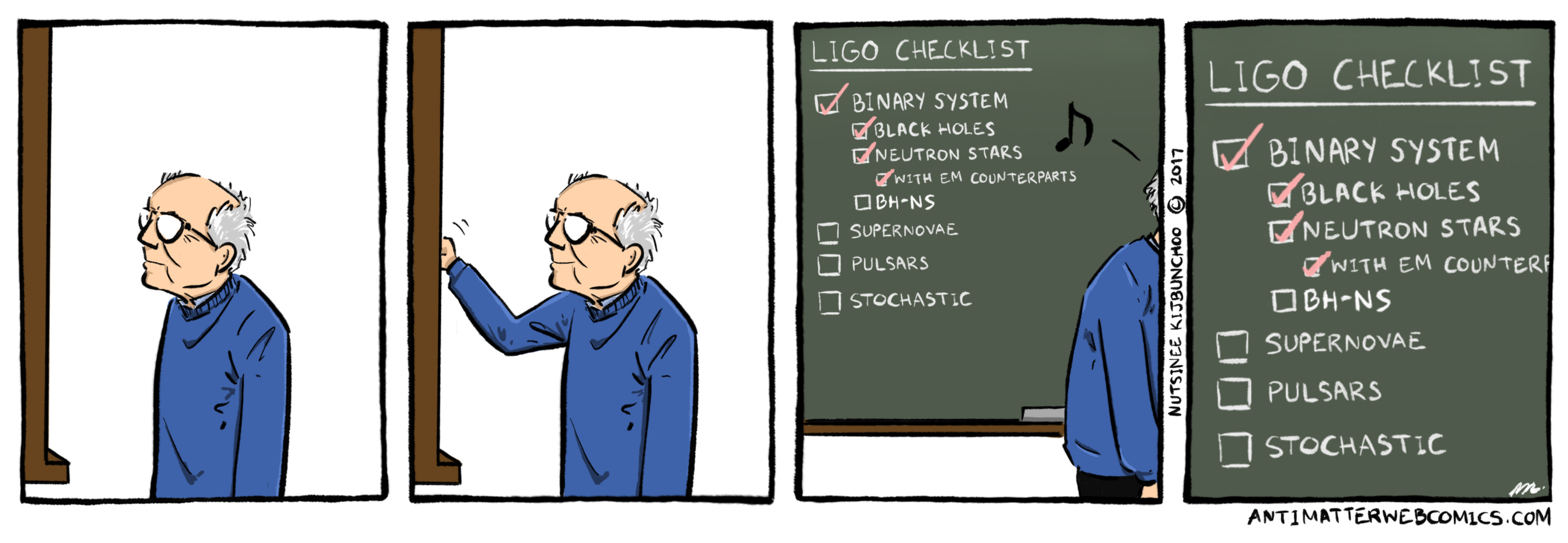

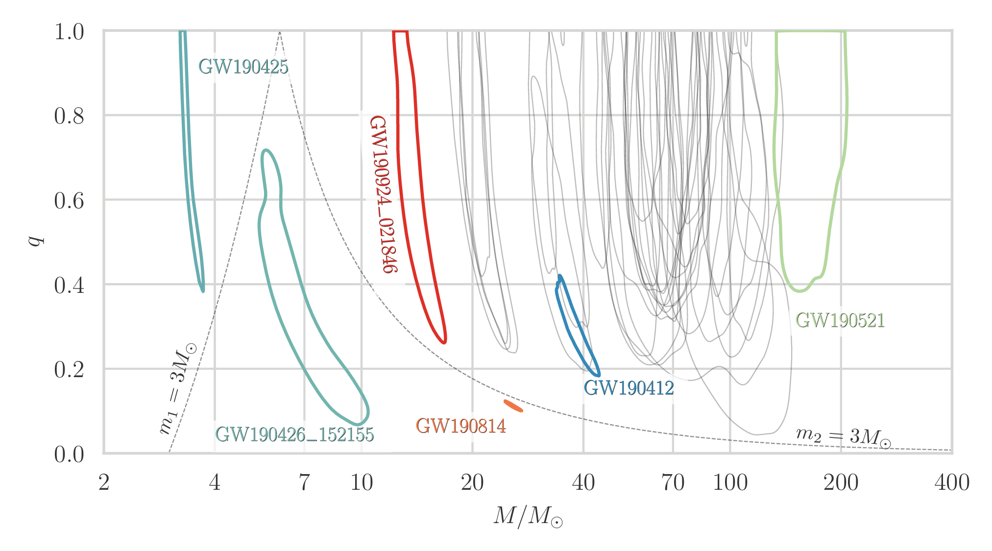


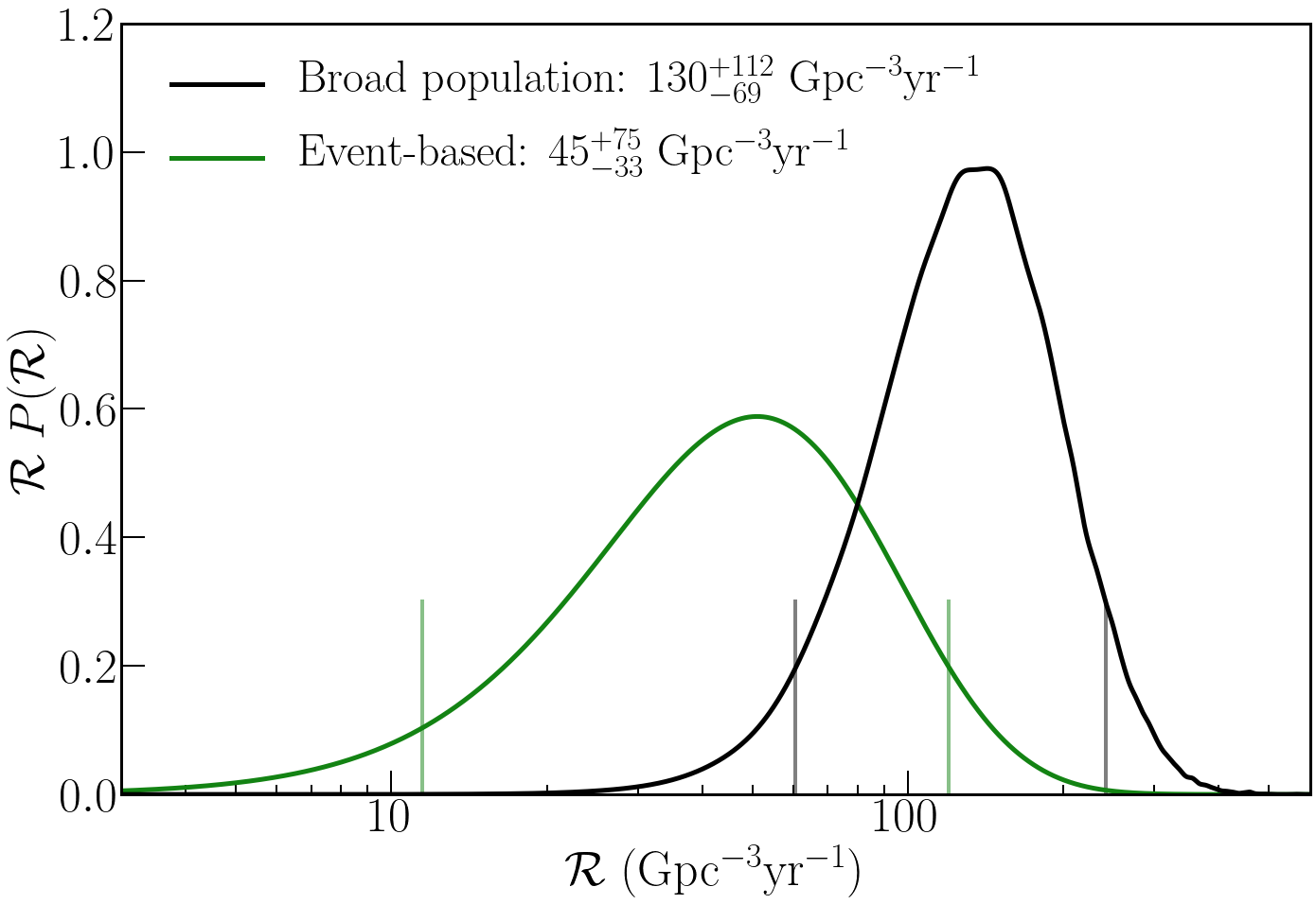


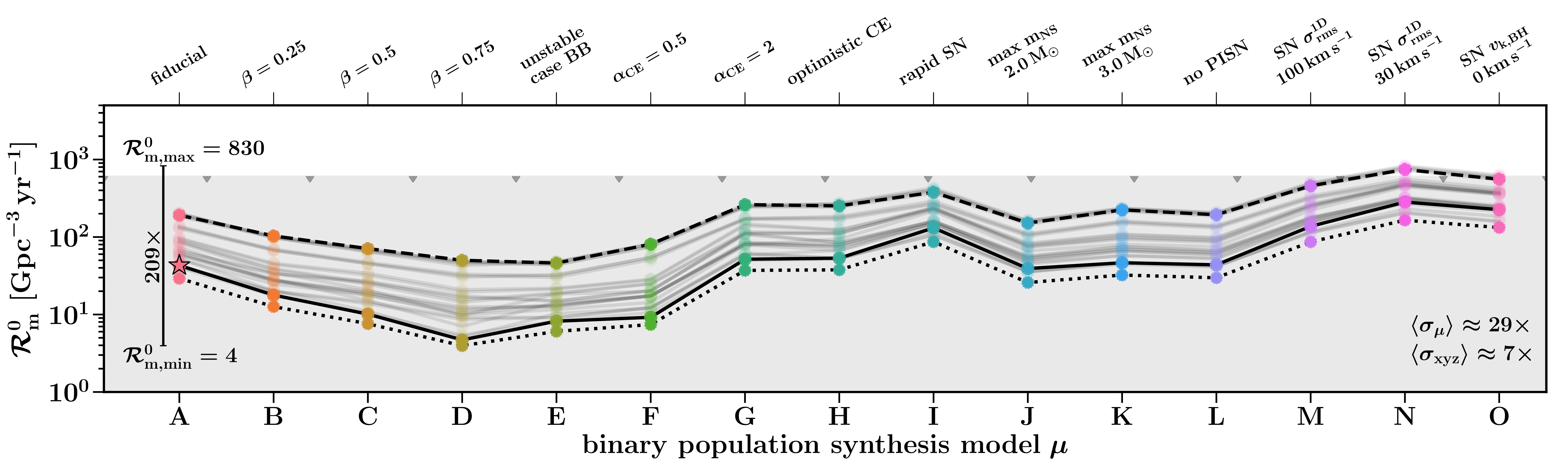


 (where our Sun has a mass of
  and
and  black hole. These massive (or
  black holes). In any case, whatever mechanism created these black holes needs to work quickly, as we know from
 . Credit:
  and
and  . Massive black holes should grow from these smaller black holes. However, we have never found one, they are the
  the merger remnant is without doubt an intermediate-mass black hole.
 and
and  . The large black hole masses extremely difficult to explain.
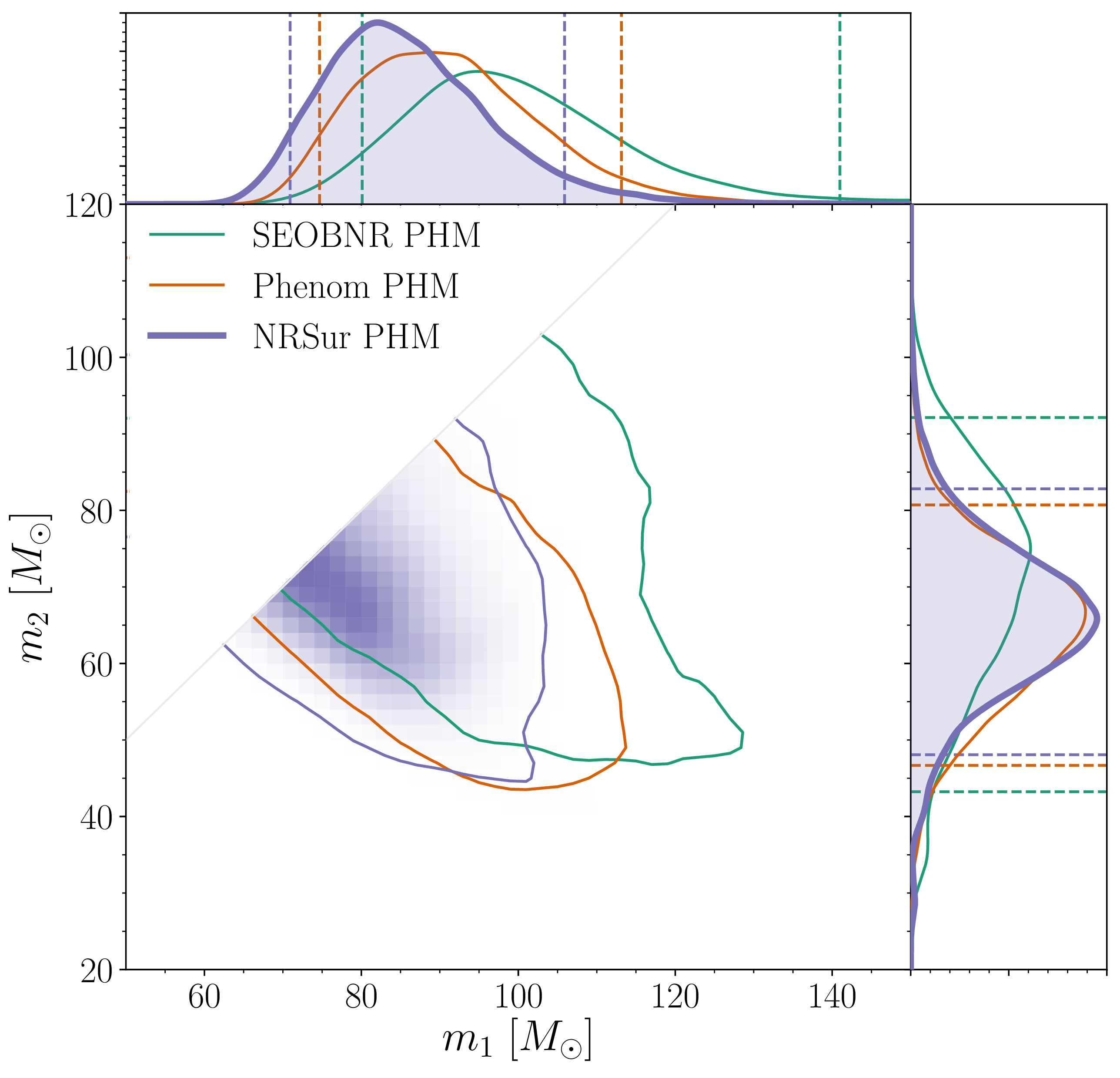
 . We show results several different waveform models and use the
  , just slightly less than the temperature of the mozerlla on that first bite of pizza, even though you should know better by now), the photons of light (gamma-rays) bouncing around inside the core become energetic enough to produce pairs of electrons and positrons [
 . If the core is between
  , the star will blast off its outer layers, possibly repeating the
  , the explosion completely destroys the star, leaving nothing behind. These stars never collapse down to a black hole, and this leaves a
  and
and  .
.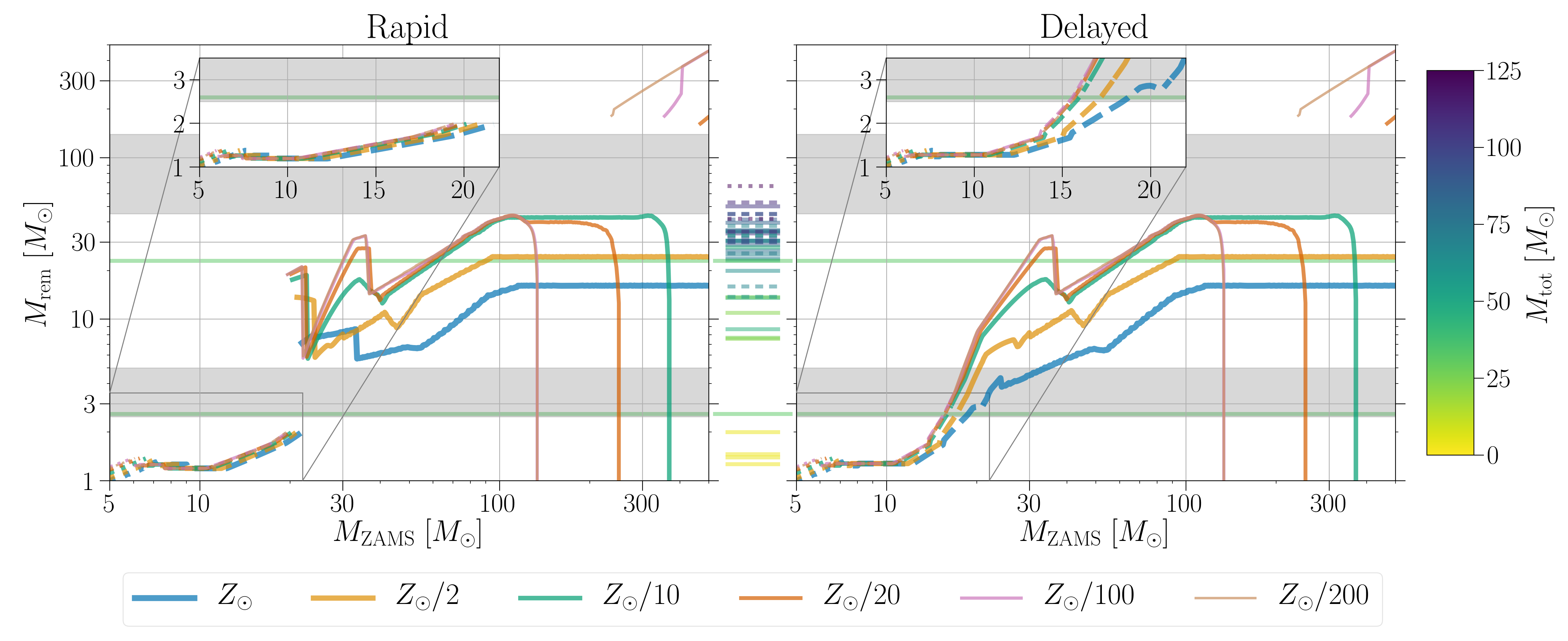
 for different initial (zero age main sequence) stellar masses
  . This is just for single stars, and ignores all the complicated things that can happen in binaries. The different coloured lines indicate different metallicities
  (higher metallicity stars lose more mass through stellar winds). The two panels are for two different supernova models. The grey bars indicate potential mass gaps: the lower core collapse mass gap (only predicted by the Rapid model) and the upper pair-instability mass gap. The tick marks in the middle are various claimed gravitational-wave source, colour-coded by the total mass of the binary
  . Figure 1 of
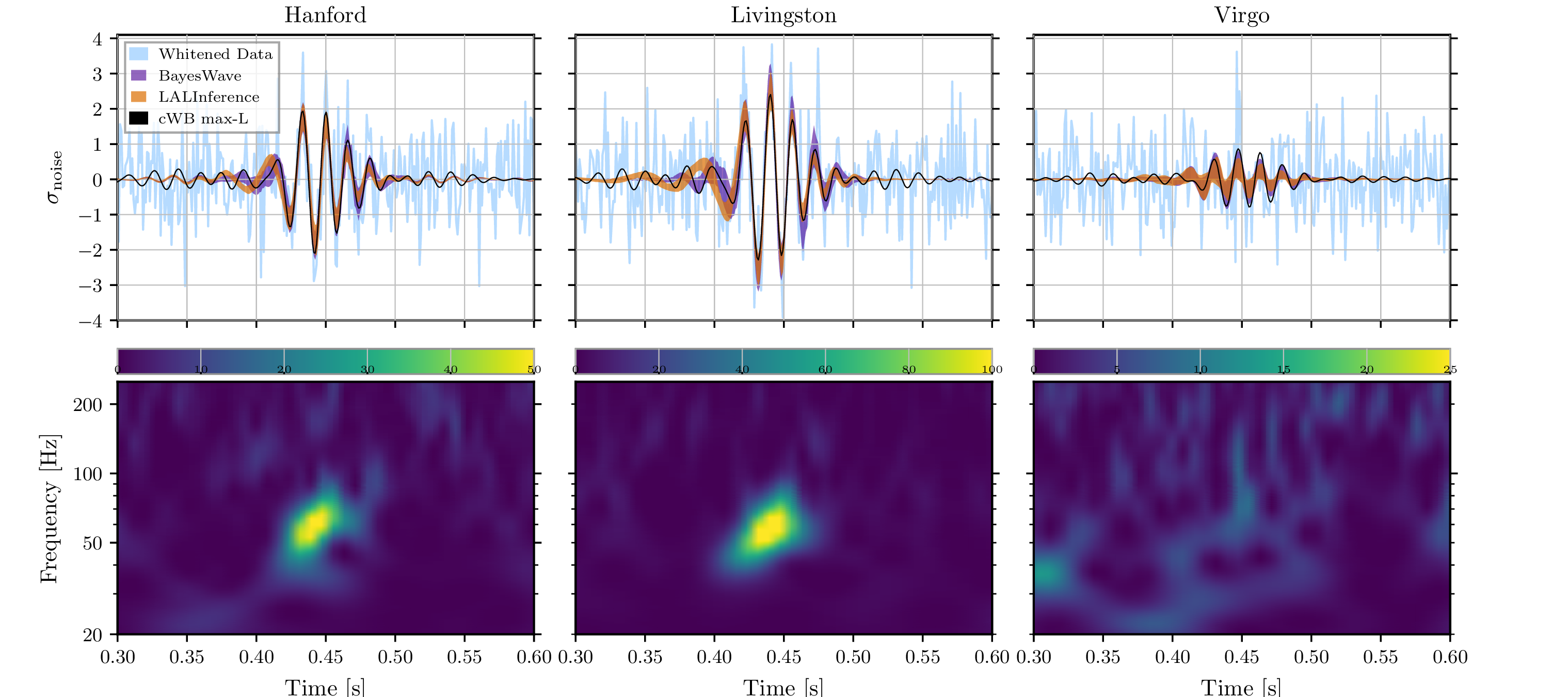
 in favour of the binary signals, so it’s probably not cosmic strings. Finally, you’ve perhaps noticed that I’ve been writing quasicircular [
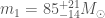 and
and  , and that the merger remnant is
  . The plot below shows the final mass as well as the spin, which is
  . For the black holes formed from the mergers of near equal mass binaries, you’d expect the final spin to be around
  .
.
 and spin
  for the final black hole. We show results several different waveform models and use the numerical relativity surrogate (NRSur PHM) as our best results. The two-dimensional shows the 90% probability contour. The dotted lines in one-dimensional plots the symmetric 90% credible interval. The mass is safely above the conventional lower limit to be considered an intermediate-mass black hole. Figure 3 of the
  . Looking at the ringdown, we get lovely consistent results trying ringdown models at different start times and including different higher order multipole moments, and all agree with the analysis of the entire signal using the quasicircular templates.
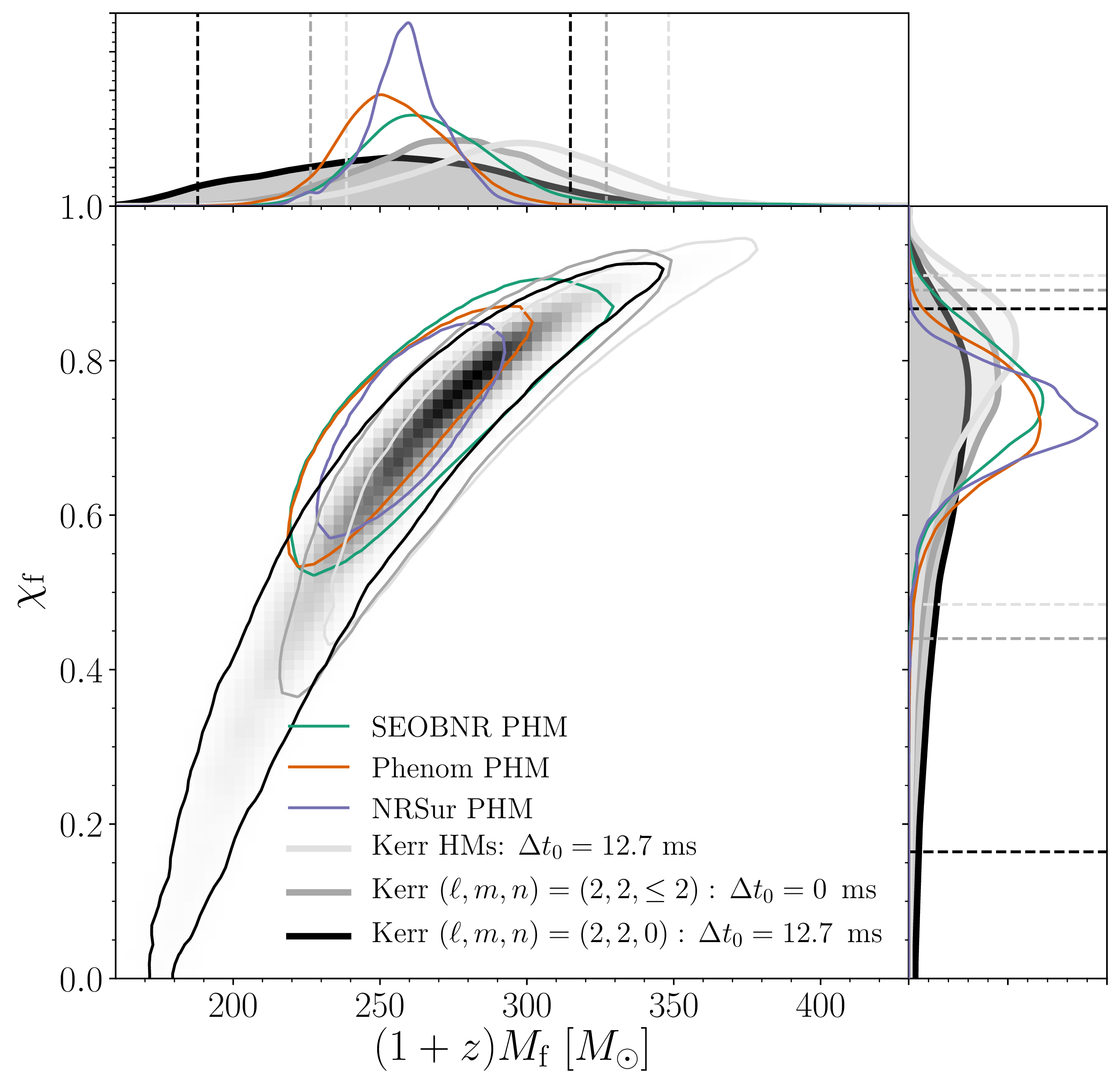
 , which goes from
  for both the spins being maximal and antialigned with the orbital angular momentum to
  for both spins being maximal and aligned with the orbital angular momentum. We find that
  , consistent with no spin, spins antialigned with each other or in the orbital plane. The result is strongly influenced by the assumed prior, we’ve not learnt much from the signal.
 , which goes from
  for no in-plane spin, to
  , but there’s support across the entire range.
 . This makes the source a good contender for the most distant gravitational wave source ever found [
 . This would be OK if sources were uniformly distributed in a non-evolving Universe, but sadly we don’t live in such a thing, and we have to take into account the expansion of the Universe, and the evolution of the galaxies and stars within it. We’ll come back to look at this when we present our catalogue of detections from the first part of the third observing run.
 , but that is extremely speculative (I’d love it if it were true). Sticking to known physics, at face value, it is hard to explain the mass of the primary black hole from our understanding of how stars evolve.
 . Predicted rates for the various formation mechanisms discussed above can be rather uncertain (kind of like how the exact value of a small bag full of
  , what if we tried
  , more like you would expect for a nuclear star cluster? We shouldn’t really be doing this, as our model is calibrated against globular cluster simulations, and nuclear star clusters have different dynamics, but we can use our results as illustrative. In this case, we find odds of about 1000:1 in favour of hierarchical mergers. This suggests that this option may be a promising one to follow, but we must moderate our results remembering that only a fraction of binaries would form in these dense environments.
 in context, if you put
 times the mass of our Sun (quoting the 90% range for parameters), and the other
  times the mass of our Sun. Neither of these masses is too surprising on their own. We know black holes come in these sizes. What is new is the ratio of the masses
 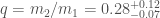 [
[
 for the two components in the binary and the effective inspiral spin
  ,
, and
and  are the spins of the two black holes [
 and
and  are the tilts angles measuring the alignment of the spins with the orbital angular momentum. The spins change orientations during the inspiral if they are not perfectly aligned with the orbital angular momentum, which is referred to as precession, but
 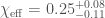 .
. .
. . This is the best measurement of
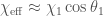 ), and similarly
  ). Combining all this information, we can actually get a good measurement of the spin of the bigger black hole. We infer that
  . This is the first time we’ve really been able to measure an individual spin!
 , where we use
  as the angles on the sphere, and
  specify the harmonic. The majority of the gravitational radiation emitted from a binary is from the
  harmonic, so we usually start with this. Larger values of
  contribute less and less. For exactly equal mass binaries with non-spinning components, only harmonics with even
  are expected to contribute a significant amount. In previous detection, we’ve not had to worry too much about the harmonics with
  , which we refer to as higher order multipole moments, as they contributed little to the signal. GW190412’s unequal masses mean that they are important here.
 , where
  is the orbital frequency. Most of the signal is emitted at twice the orbital frequency, but the emission from the higher order multipoles is at higher frequencies. If the
  multipole was a music A, then the
  multipole would correspond to an E, and if the
  showing the significance of the
  mode. This shows that the harmonic structure of gravitational waves is as expected [
 , corresponding to a travel time for the signal of around 2 billion years) using templates calculated using only the
  harmonic.
 and estimated the value of
  . A result of
  would mean that all mass ratios were equally common, while larger values would mean that binaries liked more equal mass binaries. Our analysis preferred larger values of
 to
to  , but we see that the mass ratio is still clearly unequal.
 of the time. Therefore, GW190412 is exceptional, but not completely inconsistent with our previous observations. If we repeat the calculation using the population inferred folding in GW190412, we (unsurprisingly) find it is much less unusual, with such systems being found in a set of eleven observations
  of the time. In conclusion, GW190412 is not vanilla, but is possibly raspberry ripple or Neapolitan: there’s still a trace of vanilla in there to connect it to the more usual binaries
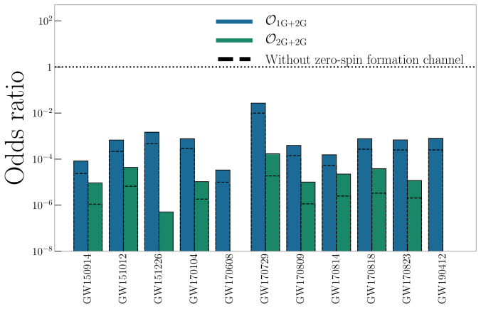
 , meaning that the mass ratio spans the entirely sensible range of
  , and those heretics who define
  , meaning that it cover the ridiculous range of
  . Within LIGO and Virgo, we have now settled on the correct convention. Many lives may have been lost, but I’m sure you’ll agree that it is a sacrifice worth making in the cause of consistent notation.
 (the Greek letter chi) and
  . After a tense negotiation, conflict was happily avoided, and we have settled on
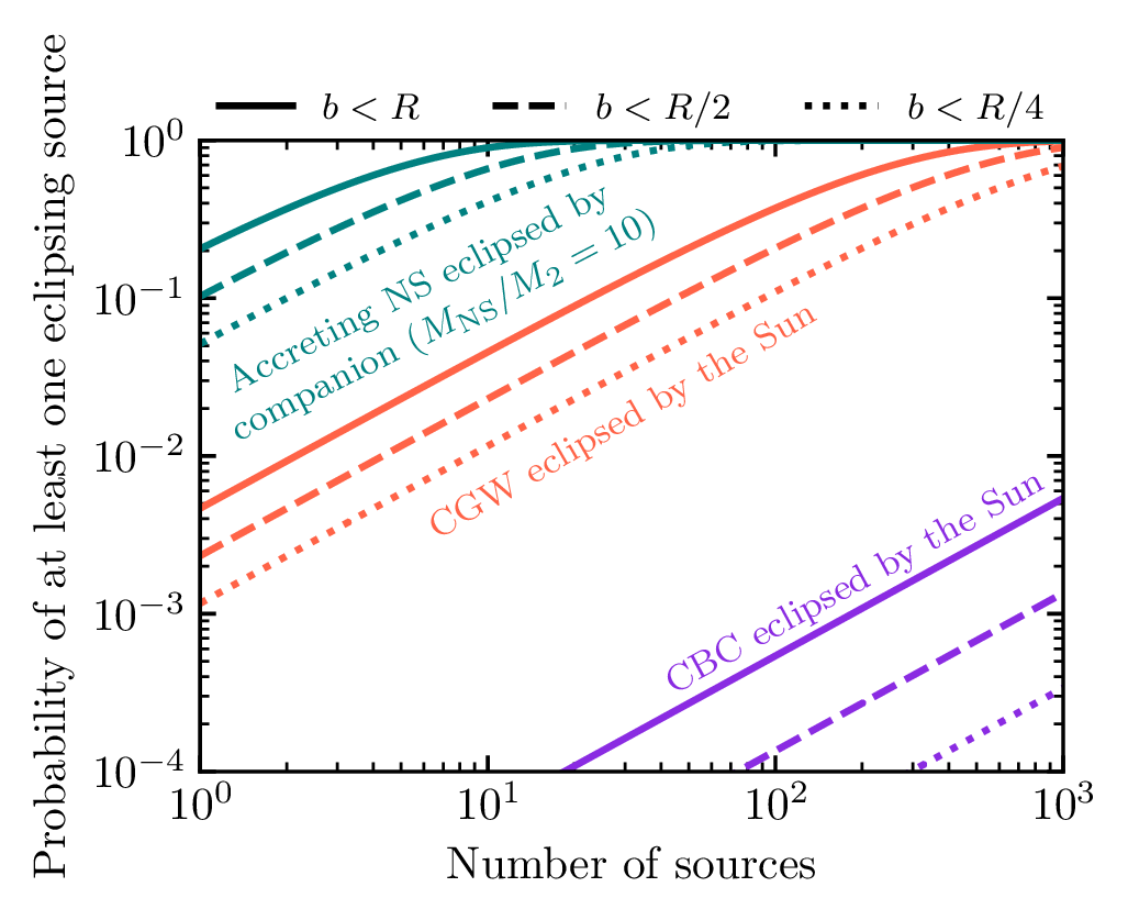
 of the centre of the star. Figure 1 of

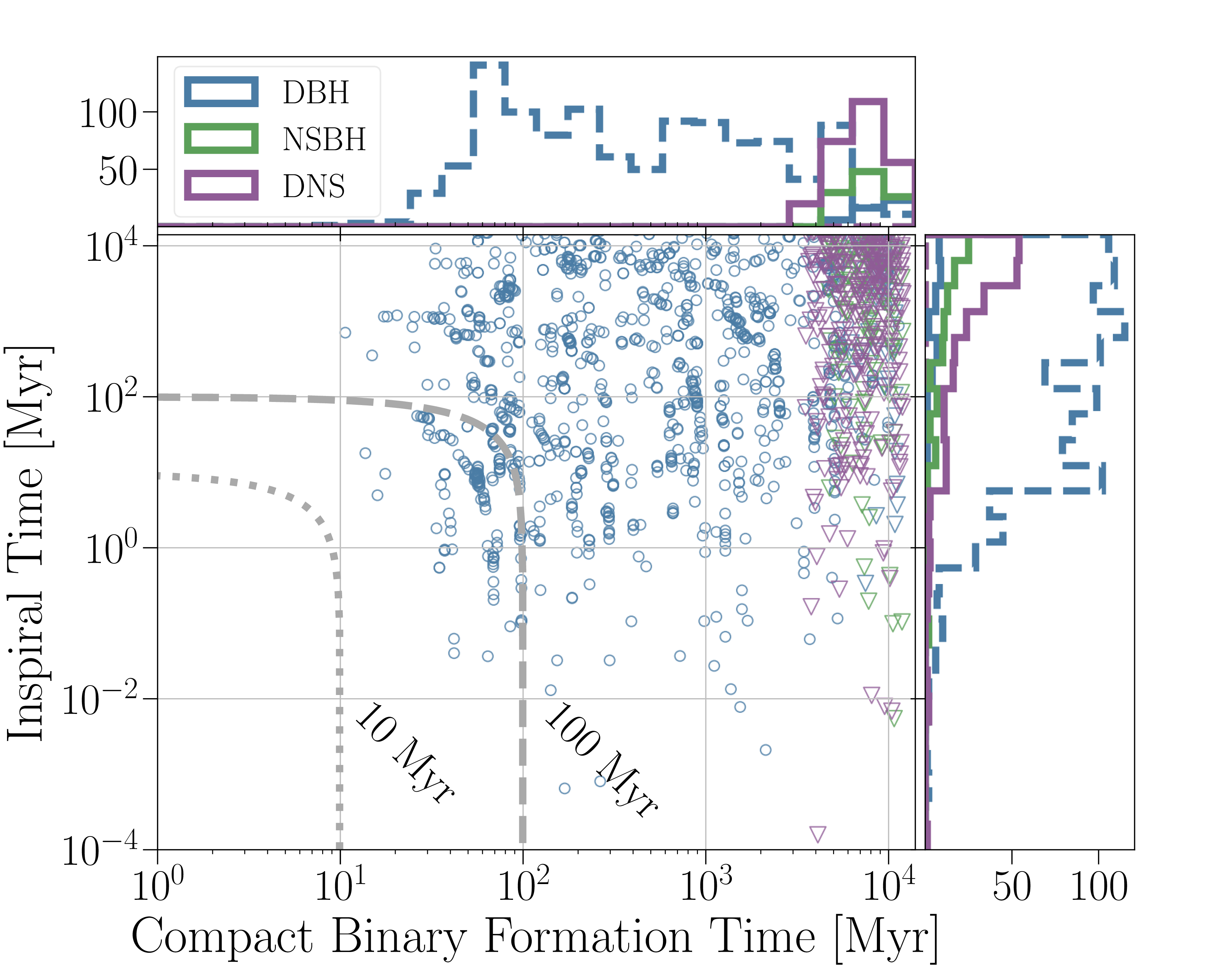

 vs inspiral time
  , and orbital separation
  ) for our population models. The lines in the left-hand plots show the bounds for a binary to enrich a cluster of a given
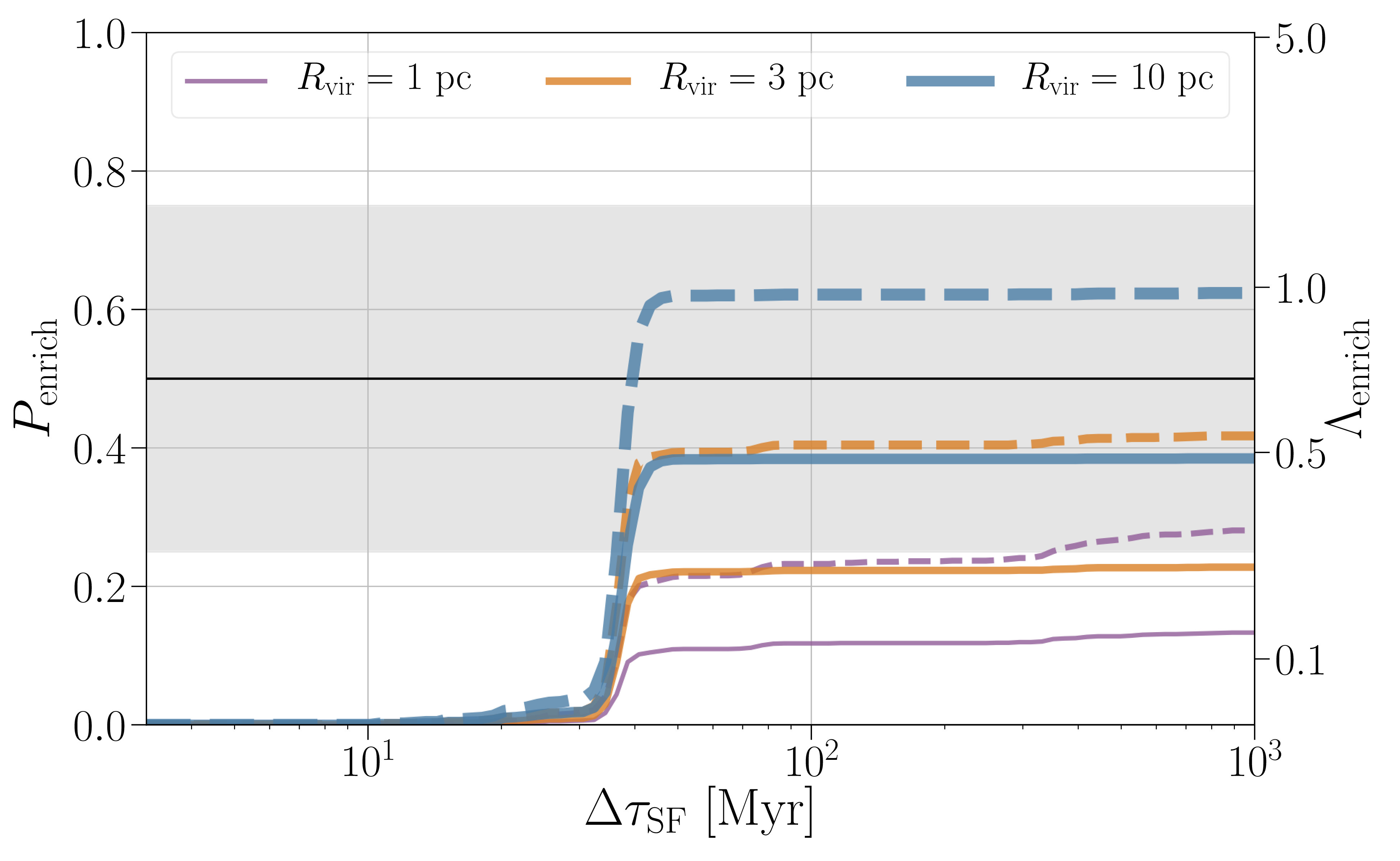
 and number of enriching binary neutron star mergers per cluster
  as a function of the timescale of star formation
  . Dashed lines are used of a cluster of a million solar masses and solid lines are used for a cluster of half this mass. Results are shown for Model D. The build up happens around the same time in different models. Figure 5 in

 solar masses (quoting the 90% range for parameters). This is larger than GW170817’s
  solar masses: we have a heavier binary.
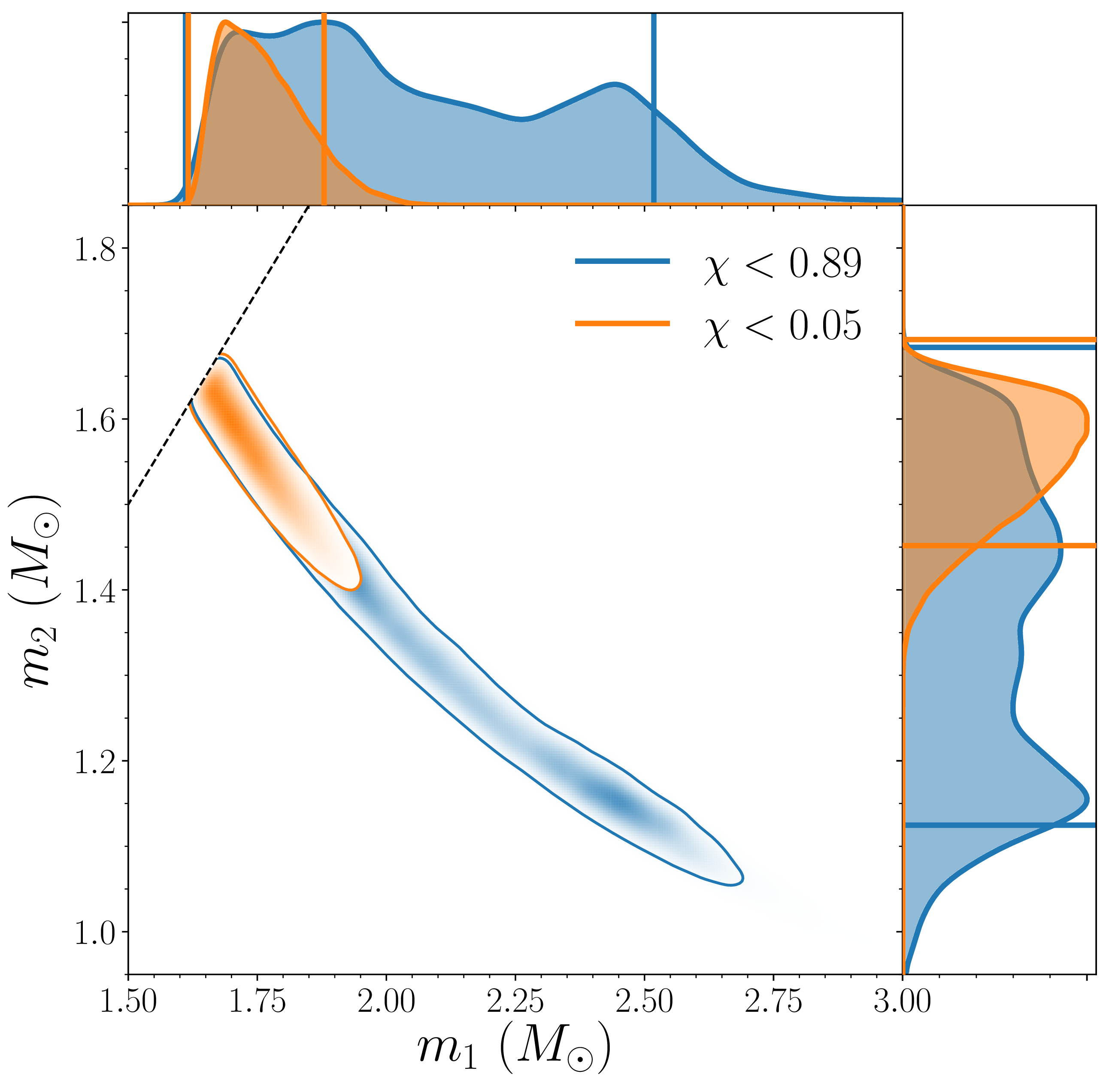
 –
– solar masses with the low-spin assumption, and
  –
– solar masses with the high-spin assumption; the lighter component has a mass
  –
– solar masses with the low-spin assumption, and
  –
– solar masses with the high-spin. These are the range of masses expected for neutron stars.
 . That means the signal was travelling across the Universe for about half a billion years. This is as many times bigger than diameter of Earth’s orbit about the Sun, as the diameter of the orbit is than the height of a LEGO brick. Space is big.
 –
– . Now, adding in the first 50 days of O3, we estimate the rate to be
  –
– , so roughly the same (which is nice) [
 , and the GW190425-like rate is lower at
  –
– . Combining the two (Assuming that binary neutron stars are all one class or the other), gives an overall rate of
  –
– , which is not too different than assuming the uniform distribution of masses.


 binary out to a redshift of about
  . The planned detector upgrade
  . That’s pretty impressive, it means we’re covering 10 billion years of history. However, the peak in the Universe’s star formation happens at around
  when the Universe was only 200 million years old and the first stars light up.
 . The plot below shows the signal from a
  binary at
  . The signal is completely undetectable at
 . If the questions can be answered with
  , then we don’t need anything beyond the currently planned A+. If we need a slightly larger
  (blue line) we can survey black holes around
  –
–
 out to redshift
  . The binaries are assumed to have equal-mass, nonspinning components. The colour scale saturates at
  . The blue curve highlights the reach at a boost factor of
  with a lower cut-off frequency of
  , we can investigate the various possibilities. The plot below shows the possible combinations of parameters which meet of requirements.

 per redshift bin as a function of A+ boost factor

 . The position is measured in terms of the
  . The
. The  . Part of Figure 1 of the


 and
and  (where
  is the mass of our Sun). The larger black hole is a contender for the most massive black hole we’ve found in a binary (the other probable contender is GW170823’s source, which has a
  black hole). We have a
  .
.

 worth of energy in gravitational waves [
 with more than 99% probability. The rest are consistent with zero. The spin distribution for GW170104 has tightened up for GW170104 as its signal-to-noise ratio has increased, and there’s less support for negative
 and the full precession model gives
  and extends to negative
  is less than 1%. In fact, we can now say that at least one spin is greater than
  at 99% probability compared with
  previously, because the full precession model likes spins in the orbital plane a bit more. Who says data analysis can’t be thrilling?
 away. That means it has travelled across the Universe for
  –
– billion years—it potentially started its journey before the Earth formed!
 means we’re looking edge-on perpendicular to the angular momentum. Part of Fig. 7 of the
 –
– for black holes between
  [
[ and
and  , and a Gaussian distribution to match electromagnetic observations. We find that these bracket the range
  –
– . This larger than are previous range, as we hadn’t considered the Gaussian distribution previously.
 . This is about a factor of 2 better than our
  instead of Model A’s
  .
. , but we can’t place a lower bound on it; the maximum black hole mass is above about
  and below about
 –
– . We infer that 99% of merging black holes have masses below
  with Model A,
  with Model B, and
 . That’s right, another power law! Since we’re only sensitive to relatively small redshifts for the masses we detect (
 ), this gives a good approximation to a range of different evolution schemes.
 , but we’re still consistent with no evolution. We might expect rate to increase as star formation was higher bach towards
  . If we can measure the time delay between forming stars and black holes merging, we could figure out what happens to these systems in the meantime.
 . We’re targeting at least
  for O3, so August 2017 gives an indication of what you can expect.
 times more energy. In conclusion, I don’t need to go on a diet.
 ,
, is the number of detections and
  is the amount of volume and time we’ve searched. You expect to detect more events if you increase the sensitivity of the detectors (and hence
  ), or observer for longer (and hence increase
  ). In our calculation, we included GW170608 in
 ,
, is the likelihood for data
  (the number of observations and their chirp mass distribution in our case),
  are our parameters (natal kick, etc.), and the angular brackets indicate the average over the population parameters. In statistics terminology, this is the variance of the
 , the common envelope efficiency
  , the Wolf–Rayet mass loss rate
  , and the luminous blue variable mass loss rate
  . There is an anticorrealtion between
  and
and 
 as following a Maxwell–Boltzmann distribution,
 ,
, is not the same as this, however, as we assume some of the material ejected by the supernova falls back, reducing the over kick. The final natal kick is
 ,
, is the fraction that falls back, taken from
  and the probability of falling in each chirp mass bin
  (we factor measurement uncertainty into this). Our observations are the the total number of detections
  and the number in each chirp mass bin
  (
( ). The likelihood is the probability of these observations given the model predictions. We can split the likelihood into two pieces, one for the rate, and one for the chirp mass distribution,
 .
.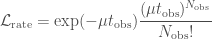 ,
, is the total observing time. For the chirp mass likelihood, we the probability of getting a number of detections in each bin, given the predicted fractions. This is given by a
 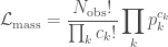 .
.![\displaystyle F_{ij} = \mu t_\mathrm{obs} \left[ \frac{1}{\mu^2} \frac{\partial \mu}{\partial \lambda_i} \frac{\partial \mu}{\partial \lambda_j} + \sum_k\frac{1}{p_k} \frac{\partial p_k}{\partial \lambda_i} \frac{\partial p_k}{\partial \lambda_j} \right]](https://s0.wp.com/latex.php?latex=%5Cdisplaystyle+F_%7Bij%7D+%3D+%5Cmu+t_%5Cmathrm%7Bobs%7D+%5Cleft%5B+%5Cfrac%7B1%7D%7B%5Cmu%5E2%7D+%5Cfrac%7B%5Cpartial+%5Cmu%7D%7B%5Cpartial+%5Clambda_i%7D%C2%A0%5Cfrac%7B%5Cpartial+%5Cmu%7D%7B%5Cpartial+%5Clambda_j%7D%C2%A0+%2B+%5Csum_k%5Cfrac%7B1%7D%7Bp_k%7D+%5Cfrac%7B%5Cpartial+p_k%7D%7B%5Cpartial+%5Clambda_i%7D%C2%A0%5Cfrac%7B%5Cpartial+p_k%7D%7B%5Cpartial+%5Clambda_j%7D+%5Cright%5D&bg=ffffff&fg=444444&s=0&c=20201002) .
. . Therefore, we can see that the measurement uncertainty defined by the inverse of the Fisher information matrix, scales on average as
  .
. and
and  are the same as their expectation values. The second-order derivatives are given by the expression we have worked out for the Fisher information matrix. Therefore, in the region around the maximum likelihood point, the Fisher information matrix encodes all the relevant information about the shape of the likelihood.
 , you’ll see that the distribution basically becomes a delta function at the maximum likelihood values. To check that our
  was large enough, we verified that higher-order derivatives were still small.