Maths-free posts for those who want to learn a little science without getting bogged down with equations. I’d encourage you to try venturing out of your comfort zone occasionally to try some of the other posts though: the maths just takes a little getting used to.
Gravitational waves and gravitational lensing are two predictions of general relativity. Gravitational waves are produced whenever masses accelerate. Gravitational lensing is produced by anything with mass. Gravitational lensing can magnify images, making it easier to spot far away things. In theory, gravitational waves can be lensed too. In this paper, we looked for evidence that GW170814 might have been lensed. (We didn’t find any, but this was my first foray into traditional astronomy).
The lensing of gravitational waves
Strong gravitational lensing magnifies a signal. A gravitational wave which has been lensed would therefore have a larger amplitude than if it had not been lensed. We infer the distance to the source of a gravitational wave from the amplitude. If we didn’t know a signal was lensed, we’d therefore think the source is much closer than it really is.
The shape of the gravitational wave encodes the properties of the source. This information is what lets us infer parameters. The example signal is GW150914 (which is fairly similar to GW170814). I made this explainer with Ban Farr and Nutsinee Kijbunchoo for the LIGO Magazine.
Mismeasuring the distance to a gravitational wave has important consequences for understanding their sources. As the gravitational wave travels across the expanding Universe, it gets stretched (redshifted) so by the time it arrives at our detectors it has a longer wavelength (and shorter frequency). If we assume that a signal came from a closer source, we’ll underestimate the amount of stretching the signal has undergone, and won’t fully correct for it. This means we’ll overestimate the masses when we infer them from the signal.
This possibility got a few people thinking when we announced our first detection, as GW150914 was heavier than previously observed black holes. Could we be seeing lensed gravitational waves?
Such strongly lensed gravitational waves should be multiply imaged. We should be able to see multiple copies of the same signal which have taken different paths from the source and then are bent by the gravity of the lens to reach us at different times. The delay time between images depends on the mass of the lens, with bigger lensing having longer delays. For galaxy clusters, it can be years.
The idea
Some of my former Birmingham colleagues who study gravitational lensing, were thinking about the possibility of having multiply imaged gravitational waves. I pointed out how difficult these would be to identify. They would come from the same part of the sky, and would have the same source parameters. However, since our uncertainties are so large for gravitational wave observations, I thought it would be tough to convince yourself that you’d seen the same signal twice [bonus note]. Lensing is expected to be rare [bonus note], so would you put your money on two signals (possibly years apart) being the same, or there just happening to be two similar systems somewhere in this huge patch of the sky?
However, if there were an optical counterpart to the merger, it would be much easier to tell that it was lensed. Since we know the location of galaxy clusters which could strongly lens a signal, we can target searches looking for counterparts at these clusters. The odds of finding anything are slim, but since this doesn’t take too much telescope time to look it’s still a gamble worth taking, as the potential pay-off would be huge.
Somehow [bonus note], I got involved in observing proposals to look for strongly lensed. We got everything in place for the last month of O2. It was just one month, so I wasn’t anticipating there being that much to do. I was very wrong.
GW170814
For GW170814 there were a couple of galaxy clusters which could serve as being strong gravitational lenses. Abell 3084 started off as the more probably, but as the sky localization for GW170814 was refined, SMACS J0304.3−4401 looked like the better bet.
Sky localization for GW170814 and the galaxy clusters Abell 3084 (filled circle), and SMACS J0304.3−4401 (open). The left plot shows the low-latency Bayestar localization (LIGO only dotted, LIGO and Virgo solid), and the right shows the refined LALInference sky maps (solid from GCN 21493, which we used for our observations, and dotted from GWTC-1). The dashed lines shows the Galactic plane. Figure 1 of Smith et al. (2019).
That’s right, absolutely nothing! [bonus note] That’s not actually too surprising. GW170814‘s source was identified as a binary black hole—assuming no lensing, its source binary had masses around 25 and 30 solar masses. We don’t expect significant electromagnetic emission from a binary black hole merger (which would make it a big discovery if found, but that is a long shot). If there source were lensed, we would have overestimated the source masses, but to get the source into the neutron star mass range would take a ridiculous amount of lensing. However, the important point is that we have demonstrated that such a search for strong lensed images is possible!
The future
In O3 [bonus notebonus note], the team has been targeting lower mass systems, where a neutron star may get mislabelled as a black hole by mistake due to a moderate amount of lensing. A false identification here could confuse our understanding of the minimum mass of a black hole, and also mean that we miss all sorts of lovely multimessenger observations, so this seems like a good plan to me.
It is possible to do a statistical analysis to calculate the probability of two signals being lensed images of each. The best attempt I’ve seen at this is Hannuksela et al. (2019). They do a nice study considering lensing by galaxies (and find nothing conclusive).
Biasing merger rates
If we included lensed events in our calculations of the merger rate density (the rate of mergers per unit volume of space), without correcting for them being lensed, we would overestimate the merger rate density. We’d assume that all our mergers came from a smaller volume of space than they actually did, as we wouldn’t know that the lensed events are being seen from further away. As long as the fraction of lensed events is small, this shouldn’t be a big problem, so we’re probably safe not to worry about it.
Slippery slope
What actually happened was my then boss, Alberto Vecchio, asked me to do some calculations based upon the sky maps for our detections in O1 as they’d only take me 5 minutes. Obviously, there were then more calculations, advice about gravitational wave alerts, feedback on observing proposals… and eventually I thought that if I’d put in this much time I might as well get a paper to show for it.
It was interesting to see how electromagnetic observing works, but I’m not sure I’d do it again.
Upper limits
Following tradition, when we don’t make a detection, we can set an upper limit on what could be there. In this case, we conclude that there is nothing to see down to an i-band magnitude of 25. This is pretty faint, about 40 million times fainter than something you could see with the naked eye (translating to visibly light). We can set such a good upper limit (compared to other follow-up efforts) as we only needed to point the telescopes at a small patch of sky around the galaxy clusters, and so we could leave them staring for a relatively long time.
O3 lensing hype
In O3, two gravitational wave candidates (S190828j and S190828l) were found just 21 minutes apart—this, for reasons I don’t entirely understand, led to much speculation that they were multiple images of a gravitationally lensed source. For a comprehensive debunking, follow this Twitter thread.
This paper, known as the Observing Scenarios Document with the Collaboration, outlines the observing plans of the ground-based detectors over the coming decade. If you want to search for electromagnetic or neutrino signals from our gravitational-wave sources, this is the paper for you. It is a living review—a document that is continuously updated.
This is the second published version, the big changes since the last version are
As you might imagine, these are quite significant updates! The first showed that we can do gravitational-wave astronomy. The second showed that we can do exactly the science this paper is about. The third makes this the first joint publication of the LIGO Scientific, Virgo and KAGRA Collaborations—hopefully the first of many to come.
I lead both this and the previous version. In my blog on the previous version, I explained how I got involved, and the long road that a collaboration must follow to get published. In this post, I’ll give an overview of the key details from the new version together with some behind-the-scenes background (working as part of a large scientific collaboration allows you to do amazing science, but it can also be exhausting). If you’d like a digest of this paper’s science, check out the LIGO science summary.
Commissioning and observing phases
The first section of the paper outlines the progression of detector sensitivities. The instruments are incredibly sensitive—we’ve never made machines to make these types of measurements before, so it takes a lot of work to get them to run smoothly. We can’t just switch them on and have them work at design sensitivity [bonus note].
Target evolution of the Advanced LIGO and Advanced Virgo detectors with time. The lower the sensitivity curve, the further away we can detect sources. The distances quoted are binary neutron star (BNS) ranges, the average distance we could detect a binary neutron star system. The BNS-optimized curve is a proposal to tweak the detectors for finding BNSs. Figure 1 of the Observing Scenarios Document.
The plots above show the planned progression of the different detectors. We had to get these agreed before we could write the later parts of the paper because the sensitivity of the detectors determines how many sources we will see and how well we will be able to localize them. I had anticipated that KAGRA would be the most challenging here, as we had not previously put together this sequence of curves. However, this was not the case, instead it was Virgo which was tricky. They had a problem with the silica fibres which suspended their mirrors (they snapped, which is definitely not what you want). The silica fibres were replaced with steel ones, but it wasn’t immediately clear what sensitivity they’d achieve and when. The final word was they’d observe in August 2017 and that their projections were unchanged. I was sceptical, but they did pull it out of the bag! We had our first clear three-detector observation of a gravitational wave 14 August 2017. Bravo Virgo!
Plausible time line of observing runs with Advanced LIGO (Hanford and Livingston), advanced Virgo and KAGRA. It is too early to give a timeline for LIGO India. The numbers above the bars give binary neutron star ranges (italic for achieved, roman for target); the colours match those in the plot above. Currently our third observing run (O3) looks like it will start in early 2019; KAGRA might join with an early sensitivity run at the end of it. Figure 2 of the Observing Scenarios Document.
Searches for gravitational-wave transients
The second section explain our data analysis techniques: how we find signals in the data, how we work out probable source locations, and how we communicate these results with the broader astronomical community—from the start of our third observing run (O3), information will be shared publicly!
The information in this section hasn’t changed much [bonus note]. There is a nice collection of references on the follow-up of different events, including GW170817 (I’d recommend my blog for more on the electromagnetic story). The main update I wanted to include was information on the detection of our first gravitational waves. It turned out to be more difficult than I imagined to come up with a plot which showed results from the five different search algorithms (two which used templates, and three which did not) which found GW150914, and harder still to make a plot which everyone liked. This plot become somewhat infamous for the amount of discussion it generated. I think we ended up with something which was a good compromise and clearly shows our detections sticking out above the background of noise.
Offline transient search results from our first observing run (O1). The plot shows the number of events found verses false alarm rate: if there were no gravitational waves we would expect the points to follow the dashed line. The left panel shows the results of the templated search for compact binary coalescences (binary black holes, binary neutron stars and neutron star–black hole binaries), the right panel shows the unmodelled burst search. GW150914, GW151226 and LVT151012 are found by the templated search; GW150914 is also seen in the burst search. Arrows indicate bounds on the significance. Figure 3 of the Observing Scenarios Document.
Observing scenarios
The third section brings everything together and looks at what the prospects are for (gravitational-wave) multimessenger astronomy during each observing run. It’s really all about the big table.
Summary of different observing scenarios with the advanced detectors. We assume a 70–75% duty factor for each instrument (including Virgo for the second scenario’s sky localization, even though it only joined our second observing run for the final month). Table 3 from the Observing Scenarios Document.
I think there are three really awesome take-aways from this
Actual binary neutron stars detected = 1. We did it!
Using the rates inferred using our observations so far (including GW170817), once we have the full five detector network of LIGO-Hanford, LIGO-Livingston, Virgo, KAGRA and LIGO-India, we could be detected 11–180 binary neutron stars a year. That something like between one a month to one every other day! I’m kind of scared…
With the five detector network the sky localization is really good. The median localization is about 9–12 square degrees, about the area the LSST could cover in a single pointing! This really shows the benefit of adding more detector to the network. The improvement comes not because a source is much better localized with five detectors than four, but because when you have five detectors you almost always have at least three detectors(the number needed to get a good triangulation) online at any moment, so you get a nice localization for pretty much everything.
In summary, the prospects for observing and localizing gravitational-wave transients are pretty great. If you are an astronomer, make the most of the quiet before O3 begins next year.
The announcement of our first multimessenger detection came between us submitting this update and us getting referee reports. We wanted an updated version of this paper, with the current details of our observing plans, to be available for our astronomer partners to be able to cite when writing their papers on GW170817.
Predictably, when the referee reports came back, we were told we really should include reference to GW170817. This type of discovery is exactly what this paper is about! There was avalanche of results surrounding GW170817, so I had to read through a lot of papers. The reference list swelled from 8 to 13 pages, but this effort was handy for my blog writing. After including all these new results, it really felt like this was version 2.5 of the Observing Scenarios, rather than version 2.
Design sensitivity
We use the term design sensitivity to indicate the performance the current detectors were designed to achieve. They are the targets we aim to achieve with Advanced LIGO, Advance Virgo and KAGRA. One thing I’ve had to try to train myself not to say is that design sensitivity is the final sensitivity of our detectors. Teams are currently working on plans for how we can upgrade our detectors beyond design sensitivity. Reaching design sensitivity will not be the end of our journey.
Binary black holes vs binary neutron stars
Our first gravitational-wave detections were from binary black holes. Therefore, when we were starting on this update there was a push to switch from focusing on binary neutron stars to binary black holes. I resisted on this, partially because I’m lazy, but mostly because I still thought that binary neutron stars were our best bet for multimessenger astronomy. This worked out nicely.
Advanced LIGO and Advanced Virgo have detected their first binary neutron star inspiral. Remarkably, this event was observed not just with gravitational waves, but also across the electromagnetic spectrum, from gamma-rays to radio. This discovery confirms the theory that binary neutron star mergers are the progenitors of short gamma-ray bursts and kilonovae, and may be the primary source of heavy elements like gold.
In this post, I’ll go through some of the story of GW170817. As for GW150914, I’ll write another post on the more technical details of our papers, once I’ve had time to catch up on sleep.
Discovery
The second observing run (O2) of the advanced gravitational-wave detectors started on 30 November 2016. The first detection came in January—GW170104. I was heavily involved in the analysis and paper writing for this. We finally finished up in June, at which point I was thoroughly exhausted. I took some time off in July [bonus note], and was back at work for August. With just one month left in the observing run, it would all be downhill from here, right?
August turned out to be the lava-filled, super-difficult final level of O2. As we have now announced, on August 14, we detected a binary black hole coalescence—GW170814. This was the first clear detection including Virgo, giving us superb sky localization. This is fantastic for astronomers searching for electromagnetic counterparts to our gravitational-wave signals. There was a flurry of excitement, and we thought that this was a fantastic conclusion to O2. We were wrong, this was just the save point before the final opponent. On August 17, we met the final, fire-ball throwing boss.
Text messages from our gravitational-wave candidate event database GraceDB. The final message is for GW170817, or as it was known at the time, G298048. It certainly caught my attention. The messages above are for GW170814, that was picked up multiple times by our search algorithms. It was a busy week.
At 1:58 pm BST my phone buzzed with a text message, an automated alert of a gravitational-wave trigger. I was obviously excited—I recall that my exact thoughts were “What fresh hell is this?” I checked our online event database and saw that it was a single-detector trigger, it was only seen by our Hanford instrument. I started to relax, this was probably going to turn out to be a glitch. The template masses, were low, in the neutron star range, not like the black holes we’ve been finding. Then I saw the false alarm rate was better than one in 9000 years. Perhaps it wasn’t just some noise after all—even though it’s difficult to estimate false alarm rates accurately online, as especially for single-detector triggers, this was significant! I kept reading. Scrolling down the page there was an external coincident trigger, a gamma-ray burst (GRB 170817A) within a couple of seconds…
Short gamma-ray bursts are some of the most powerful explosions in the Universe. I’ve always found it mildly disturbing that we didn’t know what causes them. The leading theory has been that they are the result of two neutron stars smashing together. Here seemed to be the proof.
The rapid response call was under way by the time I joined. There was a clear chirp in Hanford, you could be see it by eye! We also had data from Livingston and Virgo too. It was bad luck that they weren’t folded into the online alert. There had been a drop out in the data transfer from Italy to the US, breaking the flow for Virgo. In Livingston, there was a glitch at the time of the signal which meant the data wasn’t automatically included in the search. My heart sank. Glitches are common—check out Gravity Spy for some examples—so it was only a matter of time until one overlapped with a signal [bonus note], and with GW170817 being such a long signal, it wasn’t that surprising. However, this would complicate the analysis. Fortunately, the glitch is short and the signal is long (if this had been a high-mass binary black hole, things might not have been so smooth). We were able to exorcise the glitch. A preliminary sky map using all three detectors was sent out at 12:54 am BST. Not only did we defeat the final boss, we did a speed run on the hard difficulty setting first time [bonus note].
Spectrogram of Livingston data showing part of GW170817’s chirp (which sweeps upward in frequncy) as well as the glitch (the big blip at about ). The lower panel shows how we removed the glitch: the grey line shows gating window that was applied for preliminary results, to zero the affected times, the blue shows a fitted model of the glitch that was subtracted for final results. You can clearly see the chirp well before the glitch, so there’s no danger of it being an artefect of the glitch. Figure 2 of the GW170817 Discovery Paper
The three-detector sky map provided a great localization for the source—this preliminary map had a 90% area of ~30 square degrees. It was just in time for that night’s observations. The plot below shows our gravitational-wave localizations in green—the long band is without Virgo, and the smaller is with all three detectors—as with GW170814, Virgo makes a big difference. The blue areas are the localizations from Fermi and INTEGRAL, the gamma-ray observatories which measured the gamma-ray burst. The inset is something new…
Localization of the gravitational-wave, gamma-ray, and optical signals. The main panel shows initial gravitational-wave 90% areas in green (with and without Virgo) and gamma-rays in blue (the IPN triangulation from the time delay between Fermi and INTEGRAL, and the Fermi GBM localization). The inset shows the location of the optical counterpart (the top panel was taken 10.9 hours after merger, the lower panel is a pre-merger reference without the transient). Figure 1 of the Multimessenger Astronomy Paper.
That night, the discoveries continued. Following up on our sky location, an optical counterpart (AT 2017gfo) was found. The source is just on the outskirts of galaxy NGC 4993, which is right in the middle of the distance range we inferred from the gravitational wave signal. At around 40 Mpc, this is the closest gravitational wave source.
After this source was reported, I think about every single telescope possible was pointed at this source. I think it may well be the most studied transient in the history of astronomy. I think there are ~250 circulars about follow-up. Not only did we find an optical counterpart, but there was emission in X-ray and radio. There was a delay in these appearing, I remember there being excitement at our Collaboration meeting as the X-ray emission was reported (there was a lack of cake though).
The figure below tries to summarise all the observations. As you can see, it’s a mess because there is too much going on!
The timeline of observations of GW170817’s source. Shaded dashes indicate times when information was reported in a Circular. Solid lines show when the source was observable in a band: the circles show a comparison of brightnesses for representative observations. Figure 2 of the Multimessenger Astronomy Paper.
The observations paint a compelling story. Two neutron stars insprialled together and merged. Colliding two balls of nuclear density material at around a third of the speed of light causes a big explosion. We get a jet blasted outwards and a gamma-ray burst. The ejected, neutron-rich material decays to heavy elements, and we see this hot material as a kilonova [bonus material]. The X-ray and radio may then be the afterglow formed by the bubble of ejected material pushing into the surrounding interstellar material.
Science
What have we learnt from our results? Here are some gravitational wave highlights.
We measure several thousand cycles from the inspiral. It is the most beautiful chirp! This is the loudest gravitational wave signal yet found, beating even GW150914. GW170817 has a signal-to-noise ratio of 32, while for GW150914 it is just 24.
Time–frequency plots for GW170104 as measured by Hanford, Livingston and Virgo. The signal is clearly visible in the two LIGO detectors as the upward sweeping chirp. It is not visible in Virgo because of its lower sensitivity and the source’s position in the sky. The Livingston data have the glitch removed. Figure 1 of the GW170817 Discovery Paper.
The signal-to-noise ratios in the Hanford, Livingston and Virgo were 19, 26 and 2 respectively. The signal is quiet in Virgo, which is why you can’t spot it by eye in the plots above. The lack of a clear signal is really useful information, as it restricts where on the sky the source could be, as beautifully illustrated in the video below.
While we measure the inspiral nicely, we don’t detect the merger: we can’t tell if a hypermassive neutron star is formed or if there is immediate collapse to a black hole. This isn’t too surprising at current sensitivity, the system would basically need to convert all of its energy into gravitational waves for us to see it.
From measuring all those gravitational wave cycles, we can measure the chirp mass stupidly well. Unfortunately, converting the chirp mass into the component masses is not easy. The ratio of the two masses is degenerate with the spins of the neutron stars, and we don’t measure these well. In the plot below, you can see the probability distributions for the two masses trace out bananas of roughly constant chirp mass. How far along the banana you go depends on what spins you allow. We show results for two ranges: one with spins (aligned with the orbital angular momentum) up to 0.89, the other with spins up to 0.05. There’s nothing physical about 0.89 (it was just convenient for our analysis), but it is designed to be agnostic, and above the limit you’d plausibly expect for neutron stars (they should rip themselves apart at spins of ~0.7); the lower limit of 0.05 should safely encompass the spins of the binary neutron stars (which are close enough to merge in the age of the Universe) we have estimated from pulsar observations. The masses roughly match what we have measured for the neutron stars in our Galaxy. (The combinations at the tip of the banana for the high spins would be a bit odd).
Estimated masses for the two neutron stars in the binary. We show results for two different spin limits, is the component of the spin aligned with the orbital angular momentum. The two-dimensional shows the 90% probability contour, which follows a line of constant chirp mass. The one-dimensional plot shows individual masses; the dotted lines mark 90% bounds away from equal mass. Figure 4 of the GW170817 Discovery Paper.
If we were dealing with black holes, we’d be done: they are only described by mass and spin. Neutron stars are more complicated. Black holes are just made of warped spacetime, neutron stars are made of delicious nuclear material. This can get distorted during the inspiral—tides are raised on one by the gravity of the other. These extract energy from the orbit and accelerate the inspiral. The tidal deformability depends on the properties of the neutron star matter (described by its equation of state). The fluffier a neutron star is, the bigger the impact of tides; the more compact, the smaller the impact. We don’t know enough about neutron star material to predict this with certainty—by measuring the tidal deformation we can learn about the allowed range. Unfortunately, we also didn’t yet have good model waveforms including tides, so for to start we’ve just done a preliminary analysis (an improved analysis was done for the GW170817 Properties Paper). We find that some of the stiffer equations of state (the ones which predict larger neutron stars and bigger tides) are disfavoured; however, we cannot rule out zero tides. This means we can’t rule out the possibility that we have found two low-mass black holes from the gravitational waves alone. This would be an interesting discovery; however, the electromagnetic observations mean that the more obvious explanation of neutron stars is more likely.
From the gravitational wave signal, we can infer the source distance. Combining this with the electromagnetic observations we can do some cool things.
First, the gamma ray burst arrived at Earth 1.7 seconds after the merger. 1.7 seconds is not a lot of difference after travelling something like 85–160 million years (that’s roughly the time since the Cretaceous or Late Jurassic periods). Of course, we don’t expect the gamma-rays to be emitted at exactly the moment of merger, but allowing for a sensible range of emission times, we can bound the difference between the speed of gravity and the speed of light. In general relativity they should be the same, and we find that the difference should be no more than three parts in .
Second, we can combine the gravitational wave distance with the redshift of the galaxy to measure the Hubble constant, the rate of expansion of the Universe. Our best estimates for the Hubble constant, from the cosmic microwave background and from supernova observations, are inconsistent with each other (the most recent supernova analysis only increase the tension). Which is awkward. Gravitational wave observations should have different sources of error and help to resolve the difference. Unfortunately, with only one event our uncertainties are rather large, which leads to a diplomatic outcome.
Posterior probability distribution for the Hubble constant inferred from GW170817. The lines mark 68% and 95% intervals. The coloured bands are measurements from the cosmic microwave background (Planck) and supernovae (SHoES). Figure 1 of the Hubble Constant Paper.
Finally, we can now change from estimating upper limits on binary neutron star merger rates to estimating the rates! We estimate the merger rate density is in the range (assuming a uniform of neutron star masses between one and two solar masses). This is surprisingly close to what the Collaboration expected back in 2010: a rate of between and , with a realistic rate of . This means that we are on track to see many more binary neutron stars—perhaps one a week at design sensitivity!
Summary
Advanced LIGO and Advanced Virgo observed a binary neutron star insprial. The rest of the astronomical community has observed what happened next (sadly there are no neutrinos). This is the first time we have such complementary observations—hopefully there will be many more to come. There’ll be a huge number of results coming out over the following days and weeks. From these, we’ll start to piece together more information on what neutron stars are made of, and what happens when you smash them together (take that particle physicists).
Also: I’m exhausted, my inbox is overflowing, and I will have far too many papers to read tomorrow.
If you’re looking for the most up-to-date results regarding GW170817, check out the O2 Catalogue Paper.
Bonus notes
Inbox zero
Over my vacation I cleaned up my email. I had a backlog starting around September 2015. I think there were over 6000 which I sorted or deleted. I had about 20 left to deal with when I got back to work. GW170817 undid that. Despite doing my best to keep up, there are over a 1000 emails in my inbox…
Worst case scenario
Around the start of O2, I was asked when I expected our results to be public. I said it would depend upon what we found. If it was only high-mass black holes, those are quick to analyse and we know what to do with them, so results shouldn’t take long, now we have the first few out of the way. In this case, perhaps a couple months as we would have been generating results as we went along. However, the worst case scenario would be a binary neutron star overlapping with non-Gaussian noise. Binary neutron stars are more difficult to analyse (they are longer signals, and there are matter effects to worry about), and it would be complicated to get everyone to be happy with our results because we were doing lots of things for the first time. Obviously, if one of these happened at the end of the run, there’d be quite a delay…
I think I got that half-right. We’re done amazingly well analysing GW170817 to get results out in just two months, but I think it will be a while before we get the full O2 set of results out, as we’ve been neglecting otherthings (you’ll notice we’ve not updated our binary black hole merger rate estimate since GW170104, nor given detailed results for testing general relativity with the more recent detections).
At the time of the GW170817 alert, I was working on writing a research proposal. As part of this, I was explaining why it was important to continue working on gravitational-wave parameter estimation, in particular how to deal with non-Gaussian or non-stationary noise. I think I may be a bit of a jinx. For GW170817, the glitch wasn’t a big problem, these type of blips can be removed. I’m more concerned about the longer duration ones, which are less easy to separate out from background noise. Don’t say I didn’t warn you in O3.
Parameter estimation rota
The duty of analysing signals to infer their source properties was divided up into shifts for O2. On January 4, the time of GW170104, I was on shift with my partner Aaron Zimmerman. It was his first day. Having survived that madness, Aaron signed back up for the rota. Can you guess who was on shift for the week which contained GW170814 and GW170817? Yep, Aaron (this time partnered with the excellent Carl-Johan Haster). Obviously, we’ll need to have Aaron on rota for the entirety of O3. In preparation, he has already started on paper drafting
Methods Section: Chained ROTA member to a terminal, ignored his cries for help. Detections followed swiftly.
Especially made
The lightest elements (hydrogen, helium and lithium) we made during the Big Bang. Stars burn these to make heavier elements. Energy can be released up to around iron. Therefore, heavier elements need to be made elsewhere, for example in the material ejected from supernova or (as we have now seen) neutron star mergers, where there are lots of neutrons flying around to be absorbed. Elements (like gold and platinum) formed by this rapid neutron capture are known as r-process elements, I think because they are beloved by pirates.
A couple of weeks ago, the Nobel Prize in Physics was announced for the observation of gravitational waves. In December, the laureates will be presented with a gold (not chocolate) medal. I love the idea that this gold may have come from merging neutron stars.
Here’s one we made earlier. Credit: Associated Press/F. Vergara
Binary black hole mergers are the ultimate laboratory for testing gravity. The gravitational fields are strong, and things are moving at close to the speed of light. these extreme conditions are exactly where we expect our theories could breakdown, which is why we were so exciting by detecting gravitational waves from black hole coalescences. To accompany the first detection of gravitational waves, we performed several tests of Einstein’s theory of general relativity (it passed). This paper outlines the details of one of the tests, one that can be extended to include future detections to put Einstein’s theory to the toughest scrutiny.
One of the difficulties of testing general relativity is what do you compare it to? There are many alternative theories of gravity, but only a few of these have been studied thoroughly enough to give an concrete idea of what a binary black hole merger should look like. Even if general relativity comes out on top when compared to one alternative model, it doesn’t mean that another (perhaps one we’ve not thought of yet) can be ruled out. We need ways of looking for something odd, something which hints that general relativity is wrong, but doesn’t rely on any particular alternative theory of gravity.
The test suggested here is a consistency test. We split the gravitational-wave signal into two pieces, a low frequency part and a high frequency part, and then try to measure the properties of the source from the two parts. If general relativity is correct, we should get answers that agree; if it’s not, and there’s some deviation in the exact shape of the signal at different frequencies, we can get different answers. One way of thinking about this test is imagining that we have two experiments, one where we measure lower frequency gravitational waves and one where we measure higher frequencies, and we are checking to see if their results agree.
To split the waveform, we use a frequency around that of the last stable circular orbit: about the point that the black holes stop orbiting about each other and plunge together and merge [bonus note]. For GW150914, we used 132 Hz, which is about the same as the C an octave below middle C (a little before time zero in the simulation below). This cut roughly splits the waveform into the low frequency inspiral (where the two black hole are orbiting each other), and the higher frequency merger (where the two black holes become one) and ringdown (where the final black hole settles down).
We are fairly confident that we understand what goes on during the inspiral. This is similar physics to where we’ve been testing gravity before, for example by studying the orbits of the planets in the Solar System. The merger and ringdown are more uncertain, as we’ve never before probed these strong and rapidly changing gravitational fields. It therefore seems like a good idea to check the two independently [bonus note].
We use our parameter estimation codes on the two pieces to infer the properties of the source, and we compare the values for the mass and spin of the final black hole. We could use other sets of parameters, but this pair compactly sum up the properties of the final black hole and are easy to explain. We look at the difference between the estimated values for the mass and spin, and , if general relativity is a good match to the observations, then we expect everything to match up, and and to be consistent with zero. They won’t be exactly zero because we have noise in the detector, but hopefully zero will be within the uncertainty region [bonus note]. An illustration of the test is shown below, including one of the tests we did to show that it does spot when general relativity is not correct.
Results from the consistency test. The top panels show the outlines of the 50% and 90% credible levels for the low frequency (inspiral) part of the waveform, the high frequency (merger–ringdown) part, and the entire (inspiral–merger–ringdown, IMR) waveform. The bottom panel shows the fractional difference between the high and low frequency results. If general relativity is correct, we expect the distribution to be consistent with , indicated by the cross (+). The left panels show a general relativity simulation, and the right panel shows a waveform from a modified theory of gravity. Figure 1 of Ghosh et al. (2016).
A convenient feature of using and to test agreement with relativity, is that you can combine results from multiple observations. By averaging over lots of signals, you can reduce the uncertainty from noise. This allows you to pin down whether or not things really are consistent, and spot smaller deviations (we could get precision of a few percent after about 100 suitable detections). I look forward to seeing how this test performs in the future!
I became involved in this work as a reviewer. The LIGO Scientific Collaboration is a bit of a stickler when it comes to checking its science. We had to check that the test was coded up correctly, that the results made sense, and that calculations done and written up for GW150914 were all correct. Since most of the team are based in India [bonus note], this involved some early morning telecons, but it all went smoothly.
One of our checks was that the test wasn’t sensitive to exact frequency used to split the signal. If you change the frequency cut, the results from the two sections do change. If you lower the frequency, then there’s less of the low frequency signal and the measurement uncertainties from this piece get bigger. Conversely, there’ll be more signal in the high frequency part and so we’ll make a more precise measurement of the parameters from this piece. However, the overall results where you combine the two pieces stay about the same. You get best results when there’s a roughly equal balance between the two pieces, but you don’t have to worry about getting the cut exactly on the innermost stable orbit.
Golden binaries
In order for the test to work, we need the two pieces of the waveform to both be loud enough to allow us to measure parameters using them. This type of signals are referred to as golden. Earlier work on tests of general relativity using golden binaries has been done by Hughes & Menou (2015), and Nakano, Tanaka & Nakamura (2015). GW150914 was a golden binary, but GW151226 and LVT151012 were not, which is why we didn’t repeat this test for them.
GW150914 results
For The Event, we ran this test, and the results are consistent with general relativity being correct. The plots below show the estimates for the final mass and spin (here denoted rather than ), and the fractional difference between the two measurements. The points is at the 28% credible level. This means that if general relativity is correct, we’d expect a deviation at this level to occur around-about 72% of the time due to noise fluctuations. It wouldn’t take a particular rare realisation of noise to cause the assume true value of to be found at this probability level, so we’re not too suspicious that something is amiss with general relativity.
Results from the consistency test for The Event. The top panels final mass and spin measurements from the low frequency (inspiral) part of the waveform, the high frequency (post-inspiral) part, and the entire (IMR) waveform. The bottom panel shows the fractional difference between the high and low frequency results. If general relativity is correct, we expect the distribution to be consistent with , indicated by the cross. Figure 3 of the Testing General Relativity Paper.
The authors
Abhirup Ghosh and Archisman Ghosh were two of the leads of this study. They are both A. Ghosh at the same institution, which caused some confusion when compiling the LIGO Scientific Collaboration author list. I think at one point one of them (they can argue which) was removed as someone thought there was a mistaken duplication. To avoid confusion, they now have their full names used. This is a rare distinction on the Discovery Paper (I’ve spotted just two others). The academic tradition of using first initials plus second name is poorly adapted to names which don’t fit the typical western template, so we should be more flexible.
The world is currently going mad for Pokémon Go, so it seems like the perfect time to answer the most burning of scientific questions: what would a black hole Pokémon be like?
Black holes are, well, black. Their gravity is so strong that if you get close enough, nothing, not even light, can escape. I think that’s about as dark as you can get!
After picking Dark as a primary type, I thought Ghost was a good secondary type, since black holes could be thought of as the remains of dead stars. This also fit well with black holes not really being made of anything—they are just warped spacetime—and so are ethereal in nature. Of course, black holes’ properties are grounded in general relativity and not the supernatural.
In the games, having a secondary type has another advantage: Dark types are weak against Fighting types. In reality, punching or kicking a black hole is a Bad Idea™: it will not damage the black hole, but will certainly cause you some difficulties. However, Ghost types are unaffected by Fighting-type moves, so our black hole Pokémon doesn’t have to worry about them.
Height: 0’04″/0.1 m
Real astrophysical black holes are probably a bit too big for Pokémon games. The smallest Pokémon are currently the electric bug Joltik and fairy Flabébé, so I’ve made our black hole Pokémon the same size as these. It should comfortably fit inside a Pokéball.
Measuring the size of a black hole is actually rather tricky, since they curve spacetime. When talking about the size of a black hole, we normally think in terms of the Schwarzschild radius. Named after Karl Schwarzschild, who first calculated the spacetime of a black hole (although he didn’t realise that at the time), the Schwarzschild radius correspond to the event horizon (the point of no return) of a non-spinning black hole. It’s rather tricky to measure the distance to the centre of a black hole, so really the Schwarzschild radius gives an idea of the circumference (the distance around the edge) of the event horizon: this is 2π times the Schwarschild radius. We’ll take the height to really mean twice the Schwarzschild radius (which would be the Schwarzschild diameter, if that were actually a thing).
Weight: 7.5 × 1025 lbs/3.4 × 1025 kg
Although we made our black hole pocket-sized, it is monstrously heavy. The mass is for a black hole of the size we picked, and it is about 6 times that of the Earth. That’s still quite small for a black hole (it’s 3.6 million times less massive than the black hole that formed from GW150914’s coalescence). With this mass, our Pokémon would have a significant effect on the tides as it would quickly suck in the Earth’s oceans. Still, Pokémon doesn’t need to be too realistic.
Our black hole Pokémon would be by far the heaviest Pokémon, despite being one of the smallest. The heaviest Pokémon currently is the continent Pokémon Primal Groudon. This is 2,204.4 lbs/999.7 kg, so about 34,000,000,000,000,000,000,000 times lighter.
Within the games, having such a large weight would make our black hole Pokémon vulnerable to Grass Knot, a move which trips a Pokémon. The heavier the Pokémon, the more it is hurt by the falling over, so the more damage Grass Knot does. In the case of our Pokémon, when it trips it’s not so much that it hits the ground, but that the Earth hits it, so I think it’s fair that this hurts.
Black holes are beautifully simple, they are described just by their mass, spin and electric charge. There’s no other information you can learn about them, so I don’t think there’s any way to give them a gender. I think this is rather fitting as the sun-like Solrock is also genderless, and it seems right that stars and black holes share this.
Sticky Hold prevents a Pokémon’s item from being taken. (I’d expect wild black hole Pokémon to be sometimes found holding Stardust, from stars they have consumed). Due to their strong gravity, it is difficult to remove an object that is orbiting a black hole—a common misconception is that it is impossible to escape the pull of a black hole, this is only true if you cross the event horizon (if you replaced the Sun with a black hole of the same mass, the Earth would happily continue on its orbit as if nothing had happened).
Soundproof is an ability that protects Pokémon from sound-based moves. I picked it as a reference to sonic (or acoustic) black holes. These are black hole analogues—systems which mimic some of the properties of black holes. A sonic black hole can be made in a fluid which flows faster than its speed of sound. When this happens, sound can no longer escape this rapidly flowing region (it just gets swept away), just like light can’t escape from the event horizon or a regular black hole.
Sonic black holes are fun, because you can make them in the lab. You can them use them to study the properties of black holes—there is much excitement about possibly observing the equivalent of Hawking radiation. Predicted by Stephen Hawking (as you might guess), Hawking radiation is emitted by black holes, and could cause them to evaporate away (if they didn’t absorb more than they emit). Hawking radiation has never been observed from proper black holes, as it is very weak. However, finding the equivalent for sonic black holes might be enough to get Hawking his Nobel Prize…
The starting two moves are straightforward. Gravity is the force which governs black holes; it is gravity which pulls material in and causes the collapse of stars. I think Crunch neatly captures the idea of material being squeezed down by intense gravity.
Vacuum Wave sounds like a good description of a gravitational wave: it is a ripple in spacetime. Black holes (at least when in a binary) are great sources of gravitational waves (as GW150914 and GW151226 have shown), so this seems like a sensible move for our Pokémon to learn—although I may be biased. Why at level 16? Because Einstein first predicted gravitational waves from his theory of general relativity in 1916.
Black holes can have an electric charge, so our Pokémon should learn an Electric-type move. Charged black holes can have some weird properties. We don’t normally worry about charged black holes for two reasons. First, charged black holes are difficult to make: stuff is usually neutral overall, you don’t get a lot of similarly charged material in one place that can collapse down, and even if you did, it would quickly attract the opposite charge to neutralise itself. Second, if you did manage to make a charged black hole, it would quickly lose its charge: the strong electric and magnetic fields about the black hole would lead to the creation of charged particles that would neutralise the black hole. Discharge seems like a good move to describe this process.
Why level 18? The mathematical description of charged black holes was worked out by Hans Reissner and Gunnar Nordström, the second paper was published in 1918.
In general relativity, gravity bends spacetime. It is this warping that causes objects to move along curved paths (like the Earth orbiting the Sun). Light is affected in the same way and gets deflected by gravity, which is called gravitational lensing. This was the first experimental test of general relativity. In 1919, Arthur Eddington led an expedition to measure the deflection of light around the Sun during a solar eclipse.
Black holes, having strong gravity, can strongly lens light. The graphics from the movie Interstellar illustrate this beautifully. Below you can see how the image of the disc orbiting the black hole is distorted. The back of the disc is visible above and below the black hole! If you look closely, you can also see a bright circle inside the disc, close to the black hole’s event horizon. This is known as the light ring. It is where the path of light gets so bent, that it can orbit around and around the black hole many times. This sounds like a Light Screen to me.
Light-bending around the black hole Gargantua in Interstellar. The graphics use proper simulations of black holes, but they did fudge a couple of details to make it look extra pretty. Credit: Warner Bros./Double Negative.
These are three moves which with the most black hole-like names. Dark Void might be “black hole” after a couple of goes through Google Translate. Hyperspace Hole might be a good name for one of the higher dimensional black holes theoreticians like to play around with. (I mean, they like to play with the equations, not actually the black holes, as you’d need more than a pair of safety mittens for that). Shadow Ball captures the idea that a black hole is a three-dimensional volume of space, not just a plug-hole for the Universe. Non-rotating black holes are spherical (rotating ones bulge out at the middle, as I guess many of us do), so “ball” fits well, but they aren’t actually the shadow of anything, so it falls apart there.
I’ve picked the levels to be the masses of the two black holes which inspiralled together to produce GW150914, measured in units of the Sun’s mass, and the mass of the black hole that resulted from their merger. There’s some uncertainty on these measurements, so it would be OK if the moves were learnt a few levels either way.
When gas falls into a black hole, it often spirals around and forms into an accretion disc. You can see an artistic representation of one in the image from Instellar above. The gas swirls around like water going down the drain, making Whirlpool and apt move. As it orbits, the gas closer to the black hole is moving quicker than that further away. Different layers rub against each other, and, just like when you rub your hands together on a cold morning, they heat up. One of the ways we look for black holes is by spotting the X-rays emitted by these hot discs.
As the material spirals into a black hole, it spins it up. If a black hole swallows enough things that were all orbiting the same way, it can end up rotating extremely quickly. Therefore, I thought our black hole Pokémon should learn Rapid Spin as the same time as Whirlpool.
I picked level 63, as the solution for a rotating black hole was worked out by Roy Kerr in 1963. While Schwarzschild found the solution for a non-spinning black hole soon after Einstein worked out the details of general relativity in 1915, and the solution for a charged black hole came just after these, there’s a long gap before Kerr’s breakthrough. It was some quite cunning maths! (The solution for a rotating charged black hole was quickly worked out after this, in 1965).
Another cool thing about discs is that they could power jets. As gas sloshes around towards a black hole, magnetic fields can get tangled up. This leads to some of the material to be blasted outwards along the axis of the field. We’ve some immensely powerful jets of material, like the one below, and it’s difficult to imagine anything other than a black hole that could create such high energies! Important work on this was done by Roger Blandford and Roman Znajek in 1977, which is why I picked the level. Hyper Beam is no exaggeration in describing these jets.
Jets from Centaurus A are bigger than the galaxy itself! This image is a composite of X-ray (blue), microwave (orange) and visible light. You can see the jets pushing out huge bubbles above and below the galaxy. We think the jets are powered by the galaxy’s central supermassive black hole. Credit: ESO/WFI/MPIfR/APEX/NASA/CXC/CfA/A.Weiss et al./R.Kraft et al.
After using Hyper Beam, a Pokémon must recharge for a turn. It’s an exhausting move. A similar thing may happen with black holes. If they accrete a lot of stuff, the radiation produced by the infalling material blasts away other gas and dust, cutting off the black hole’s supply of food. Black holes in the centres of galaxies may go through cycles of feeding, with discs forming, blowing away the surrounding material, and then a new disc forming once everything has settled down. This link between the black hole and its environment may explain why we see a trend between the size of supermassive black holes and the properties of their host galaxies.
To finish off, since black holes are warped spacetime, a space move and a time move. Relativity say that space and time are two aspects of the same thing, so these need to be learnt together.
It’s rather tricky to imagine space and time being linked. Wibbly-wobbly, timey-wimey, spacey-wacey stuff gets quickly gets befuddling. If you imagine just two space dimension (forwards/backwards and left/right), then you can see how to change one to the other by just rotating. If you turn to face a different way, you can mix what was left to become forwards, or to become a bit of right and a bit of forwards. Black holes sort of do the same thing with space and time. Normally, we’re used to the fact that we a definitely travelling forwards in time, but if you stray beyond the event horizon of a black hole, you’re definitely travelling towards the centre of the black hole in the same inescapable way. Black holes are the masters when it comes to manipulating space and time.
There we have it, we can now sleep easy knowing what a black hole Pokémon would be like. Well almost, we still need to come up with a name. Something resembling a pun would be traditional. Suggestions are welcome. The next games in the series are Pokémon Sun and Pokémon Moon. Perhaps with this space theme Nintendo might consider a black hole Pokémon too?
I love collecting things, there’s something extremely satisfying about completing a set. I suspect that this is one of the alluring features of Pokémon—you’ve gotta catch ’em all. The same is true of black hole hunting. Currently, we know of stellar-mass black holes which are a few times the mass of our Sun, up to a few tens of the mass of our Sun (the black holes of GW150914 are the biggest yet to be observed), and we know of supermassive black holes, which are ten thousand to ten billion times the mass our Sun. However, we are missing intermediate-mass black holes which lie in the middle. We have Charmander and Charizard, but where is Charmeleon? The elusive ones are always the most satisfying to capture.
Adorable black hole (available for adoption). I’m sure this could be a Pokémon. It would be a Dark type. Not that I’ve given it that much thought…
Intermediate-mass black holes have evaded us so far. We’re not even sure that they exist, although that would raise questions about how you end up with the supermassive ones (you can’t just feed the stellar-mass ones lots of rare candy). Astronomers have suggested that you could spot intermediate-mass black holes in globular clusters by the impact of their gravity on the motion of other stars. However, this effect would be small, and near impossible to conclusively spot. Another way (which I’ve discussed before), would to be to look at ultra luminous X-ray sources, which could be from a disc of material spiralling into the black hole. However, it’s difficult to be certain that we understand the source properly and that we’re not misclassifying it. There could be one sure-fire way of identifying intermediate-mass black holes: gravitational waves.
The frequency of gravitational waves depend upon the mass of the binary. More massive systems produce lower frequencies. LIGO is sensitive to the right range of frequencies for stellar-mass black holes. GW150914 chirped up to the pitch of a guitar’s open B string (just below middle C). Supermassive black holes produce gravitational waves at too low frequency for LIGO (a space-based detector would be perfect for these). We might just be able to detect signals from intermediate-mass black holes with LIGO.
In a recent paper, a group of us from Birmingham looked at what we could learn from gravitational waves from the coalescence of an intermediate-mass black hole and a stellar-mass black hole [bonus note]. We considered how well you would be able to measure the masses of the black holes. After all, to confirm that you’ve found an intermediate-mass black hole, you need to be sure of its mass.
The signals are extremely short: we only can detect the last bit of the two black holes merging together and settling down as a final black hole. Therefore, you might think there’s not much information in the signal, and we won’t be able to measure the properties of the source. We found that this isn’t the case!
We considered a set of simulated signals, and analysed these with our parameter-estimation code [bonus note]. Below are a couple of plots showing the accuracy to which we can infer a couple of different mass parameters for binaries of different masses. We show the accuracy of measuring the chirp mass (a much beloved combination of the two component masses which we are usually able to pin down precisely) and the total mass .
Measured chirp mass for systems of different total masses. The shaded regions show the 90% credible interval and the dashed lines show the true values. The mass ratio is the mass of the stellar-mass black hole divided by the mass of the intermediate-mass black hole. Figure 1 of Haster et al. (2016).
Measured total mass for systems of different total masses. The shaded regions show the 90% credible interval and the dashed lines show the true values. Figure 2 of Haster et al. (2016).
For the lower mass systems, we can measure the chirp mass quite well. This is because we get a little information from the part of the gravitational wave from when the two components are inspiralling together. However, we see less and less of this as the mass increases, and we become more and more uncertain of the chirp mass.
The total mass isn’t as accurately measured as the chirp mass at low masses, but we see that the accuracy doesn’t degrade at higher masses. This is because we get some constraints on its value from the post-inspiral part of the waveform.
We found that the transition from having better fractional accuracy on the chirp mass to having better fractional accuracy on the total mass happened when the total mass was around 200–250 solar masses. This was assuming final design sensitivity for Advanced LIGO. We currently don’t have as good sensitivity at low frequencies, so the transition will happen at lower masses: GW150914 is actually in this transition regime (the chirp mass is measured a little better).
Given our uncertainty on the masses, when can we conclude that there is an intermediate-mass black hole? If we classify black holes with masses more than 100 solar masses as intermediate mass, then we’ll be able to say to claim a discovery with 95% probability if the source has a black hole of at least 130 solar masses. The plot below shows our inferred probability of there being an intermediate-mass black hole as we increase the black hole’s mass (there’s little chance of falsely identifying a lower mass black hole).
Probability that the larger black hole is over 100 solar masses (our cut-off mass for intermediate-mass black holes ). Figure 7 of Haster et al. (2016).
Gravitational-wave observations could lead to a concrete detection of intermediate mass black holes if they exist and merge with another black hole. However, LIGO’s low frequency sensitivity is important for detecting these signals. If detector commissioning goes to plan and we are lucky enough to detect such a signal, we’ll finally be able to complete our set of black holes.
The coalescence of an intermediate-mass black hole and a stellar-mass object (black hole or neutron star) has typically been known as an intermediate mass-ratio inspiral (an IMRI). This is similar to the name for the coalescence of a a supermassive black hole and a stellar-mass object: an extreme mass-ratio inspiral (an EMRI). However, my colleague Ilya has pointed out that with LIGO we don’t really see much of the intermediate-mass black hole and the stellar-mass black hole inspiralling together, instead we see the merger and ringdown of the final black hole. Therefore, he prefers the name intermediate mass-ratio coalescence (or IMRAC). It’s a better description of the signal we measure, but the acronym isn’t as good.
Parameter-estimation runs
The main parameter-estimation analysis for this paper was done by Zhilu, a summer student. This is notable for two reasons. First, it shows that useful research can come out of a summer project. Second, our parameter-estimation code installed and ran so smoothly that even an undergrad with no previous experience could get some useful results. This made us optimistic that everything would work perfectly in the upcoming observing run (O1). Unfortunately, a few improvements were made to the code before then, and we were back to the usual level of fun in time for The Event.
The week beginning February 8th was a big one for the LIGO and Virgo Collaborations. You might remember something about a few papers on the merger of a couple of black holes; however, those weren’t the only papers we published that week. In fact, they are not even (currently) the most cited…
Its content is a mix of a schedule for detector commissioning and an explanation of data analysis. It is a rare paper that spans both the instrumental and data-analysis sides of the Collaboration.
It is a living review: it is intended to be periodically updated as we get new information.
There is also one further point of interest for me: I was heavily involved in producing this latest version.
In this post I’m going to give an outline of the paper’s content, but delve a little deeper into the story of how this paper made it to print.
The Observing Scenarios
The paper is divided up into four sections.
It opens, as is traditional, with the introduction. This has no mentions of windows, which is a good start.
Section 2 is the instrumental bit. Here we give a possible timeline for the commissioning of the LIGO and Virgo detectors and a plausible schedule for our observing runs.
Next we talk about data analysis for transient (short) gravitational waves. We discuss detection and then sky localization.
Finally, we bring everything together to give an estimate of how well we expect to be able to locate the sources of gravitational-wave signals as time goes on.
Packaged up, the paper is useful if you want to know when LIGO and Virgo might be observing or if you want to know how we locate the source of a signal on the sky. The aim was to provide a guide for those interested in multimessenger astronomy—astronomy where you rely on multiple types of signals like electromagnetic radiation (light, radio, X-rays, etc.), gravitational waves, neutrinos or cosmic rays.
The development of the detectors’ sensitivity is shown below. It takes many years of tweaking and optimising to reach design sensitivity, but we don’t wait until then to do some science. It’s just as important to practise running the instruments and analysing the data as it is to improve the sensitivity. Therefore, we have a series of observing runs at progressively higher sensitivity. Our first observing run (O1), featured just the two LIGO detectors, which were towards the better end of the expected sensitivity.
Plausible evolution of the Advanced LIGO and Advanced Virgo detectors with time. The lower the sensitivity curve, the further away we can detect sources. The distances quoted are ranges we could observe binary neutrons stars (BNSs) to. The BNS-optimized curve is a proposal to tweak the detectors for finding BNSs. Fig. 1 of the Observing Scenarios Document.
It’s difficult to predict exactly how the detectors will progress (we’re doing many things for the first time ever), but the plot above shows our current best plan.
I’ll not go into any more details about the science in the paper as I’ve already used up my best ideas writing the LIGO science summary.
If you’re particularly interested in sky localization, you might like to check out the data releases for studies using (simulated) binary neutron star and burst signals. The binary neutron star analysis is similar to that we do for any compact binary coalescence (the merger of a binary containing neutron stars or black holes), and the burst analysis works more generally as it doesn’t require a template for the expected signal.
The path to publication
Now, this is the story of how a Collaboration paper got published. I’d like to take a minute to tell you how I became responsible for updating the Observing Scenarios…
In the beginning
The Observing Scenarios has its origins long before I joined the Collaboration. The first version of the document I can find is from July 2012. Amongst the labyrinth of internal wiki pages we have, the earliest reference I’ve uncovered was from August 2012 (the plan was to have a mature draft by September). The aim was to give a road map for the advanced-detector era, so the wider astronomical community would know what to expect.
I imagine it took a huge effort to bring together all the necessary experts from across the Collaboration to sit down and write the document.
Any document detailing our plans would need to be updated regularly as we get a better understanding of our progress on commissioning the detectors (and perhaps understanding what signals we will see). Fortunately, there is a journal that can cope with just that: Living Reviews in Relativity. Living Reviews is designed so that authors can update their articles so that they never become (too) out-of-date.
A version was submitted to Living Reviews early in 2013, around the same time as a version was posted to the arXiv. We had referee reports (from two referees), and were preparing to resubmit. Unfortunately, Living Reviews suspended operations before we could. However, work continued.
Updating sky localization
I joined the LIGO Scientific Collaboration when I started at the University of Birmingham in October 2013. I soon became involved in a variety of activities of the Parameter Estimation group (my boss, Alberto Vecchio, is the chair of the group).
Sky localization was a particularly active area as we prepared for the first runs of Advanced LIGO. The original version of the Observing Scenarios Document used a simple approximate means of estimating sky localization, using just timing triangulation (it didn’t even give numbers for when we only had two detectors running). We knew we could do better.
We had all the code developed, but we needed numbers for a realistic population of signals. I was one of the people who helped running the analyses to get these. We had the results by the summer of 2014; we now needed someone to write up the results. I have a distinct recollection of there being silence on our weekly teleconference. Then Alberto asked me if I would do it? I said yes: it would probably only take me a week or two to write a short technical note.
Numbers in hand, it was time to update the Observing Scenarios. Even if things were currently on hold with Living Reviews, we could still update the arXiv version. I thought it would be easiest if I put them in, with a little explanation, myself. I compiled a draft and circulated in the Parameter Estimation group. Then it was time to present to the Data Analysis Council.
The Data Analysis Council either sounds like a shadowy organisation orchestrating things from behind the scene, or a place where people bicker over trivial technical issues. In reality it is a little of both. This is the body that should coordinate all the various bits of analysis done by the Collaboration, and they have responsibility for the Observing Scenarios Document. I presented my update on the last call before Christmas 2014. They were generally happy, but said that the sky localization on the burst side needed updating too! There was once again a silence on the call when it came to the question of who would finish off the document. The Observing Scenarios became my responsibility.
(I had though that if I helped out with this Collaboration paper, I could take the next 900 off. This hasn’t worked out.)
The review
With some help from the Burst group (in particular Reed Essick, who had lead their sky localization study), I soon had a new version with fully up-to-date sky localization. This was ready for our March Collaboration meeting. I didn’t go (I was saving my travel budget for the summer), so Alberto presented on my behalf. It was now agreed that the document should go through internal review.
It’s this which I really want to write about. Peer review is central to modern science. New results are always discussed by experts in the community, to try to understand the value of the work; however, peer review is formalised in the refereeing of journal articles, when one or more (usually anonymous) experts examine work before it can be published. There are many ups and down with this… For Collaboration papers, we want to be sure that things are right before we share them publicly. We go through internal peer review. In my opinion this is much more thorough than journal review, and this shows how seriously the Collaboration take their science.
Unfortunately, setting up the review was also where we hit a hurdle—it took until July. I’m not entirely sure why there was a delay: I suspect it was partly because everyone was busy assembling things ahead of O1 and partly because there were various discussions amongst the high-level management about what exactly we should be aiming for. Working as part of a large collaboration can mean that you get to be involved in wonderful science, but it can means lots of bureaucracy and politics. However, in the intervening time, Living Reviews was back in operation.
The review team consisted of five senior people, each of whom had easily five times as much experience as I do, with expertise in each of the areas covered in the document. The chair of the review was Alan Weinstein, head of the Caltech LIGO Laboratory Astrophysics Group, who has an excellent eye for detail. Our aim was to produce the update for the start of O1 in September. (Spolier: We didn’t make it)
The review team discussed things amongst themselves and I got the first comments at the end of August. The consensus was that we should not just update the sky localization, but update everything too (including the structure of the document). This precipitated a flurry of conversations with the people who organise the schedules for the detectors, those who liaise with our partner astronomers on electromagnetic follow-up, and everyone who does sky localization. I was initially depressed that we wouldn’t make our start of O1 deadline; however, then something happened that altered my perspective.
On September 14, four days before the official start of O1, we made a detection. GW150914 would change everything.
First, we could no longer claim that binary neutron stars were expected to be our most common source—instead they became the source we expect would most commonly have an electromagnetic counterpart.
Second, we needed to be careful how we described engineering runs. GW150914 occurred in our final engineering run (ER8). Practically, there was difference between the state of the detector then and in O1. The point of the final engineering run was to get everything running smoothly so all we needed to do at the official start of O1 was open the champagne. However, we couldn’t make any claims about being able to make detections during engineering runs without being krass and letting the cat out of the bag. I’m rather pleased with the sentence
Engineering runs in the commissioning phase allow us to understand our detectors and analyses in an observational mode; these are not intended to produce astrophysical results, but that does not preclude the possibility of this happening.
I don’t know if anyone noticed the implication. (Checking my notes, this was in the September 18 draft, which shows how quickly we realised the possible significance of The Event).
Finally, since the start of observations proved to be interesting, and because the detectors were running so smoothly, it was decided to extend O1 from three months to four so that it would finish in January. No commissioning was going to be done over the holidays, so it wouldn’t affect the schedule. I’m not sure how happy the people who run the detectors were about working over this period, but they agreed to the plan. (No-one asked if we would be happy to run parameter estimation over the holidays).
After half-a-dozen drafts, the review team were finally happy with the document. It was now October 20, and time to proceed to the next step of review: circulation to the Collaboration.
Collaboration papers go through a sequence of stages. First they are circulated to the everyone for comments. This can be pointing out typos, suggesting references or asking questions about the analysis. This lasts two weeks. During this time, the results must also be presented on a Collaboration-wide teleconference. After comments are addressed, the paper is sent for examination Executive Committees of the LIGO and Virgo Collaborations. After approval from them (and the review team check any changes), the paper is circulated to the Collaboration again for any last comments and checking of the author list. At the same time it is sent to the Gravitational Wave International Committee, a group of all the collaborations interested in gravitational waves. This final stage is a week. Then you can you can submit the paper.
Peer review for the journal doesn’t seem to arduous in comparison does it?
Since things were rather busy with all the analysis of GW150914, the Observing Scenario took a little longer than usual to clear all these hoops. I presented to the Collaboration on Friday 13 November. (This was rather unlucky as I was at a workshop in Italy and I had to miss the tour of the underground Laboratori Nazionali del Gran Sasso). After addressing comments from everyone (the Executive Committees do read things carefully), I got the final sign-off to submit December 21. At least we made it before the end of O1.
Good things come…
This may sound like a tale of frustration and delay. However, I hope that it is more than that, and it shows how careful the Collaboration is. The Observing Scenarios is really a review: it doesn’t contain new science. The updated sky localization results are from studies which have appeared in peer-reviewed journals, and are based upon codes that have been separately reviewed. Despite this, every statement was examined and every number checked and rechecked, and every member of the Collaboration had opportunity to examine the results and comment on the document.
I guess this attention to detail isn’t surprising given that our work is based on measuring a change in length of one part in 1,000,000,000,000,000,000,000.
Since this is how we treat review articles, can you imagine how much scrutiny the Discovery Paper had? Everything had at least one extra layer of review, every number had to be signed-off individually by the appropriate review team, and there were so many comments on the paper that the editors had to switch to using a ticketing system we normally use for tracking bugs in our software. This level of oversight helped me to sleep a little more easily: there are six numbers in the abstract alone I could have potentially messed up.
Had a nightmare that all my numbers changed when I reran my analysis. Went back to sleep after remembering dreams aren't reviewed yet.
Of course, all this doesn’t mean we can’t make mistakes…
Looking forward
The Living Reviews version was accepted January 22, just after the end of O1. We made had to make a couple of tweaks to correct tenses. The final version appeared February 8, in time to be the last paper of the pre-discovery era.
It is now time to be thinking about the next update! There are certainly a few things on the to-do list (perhaps even some news on LIGO-India). We are having a Collaboration meeting in a couple of weeks’ time, so hopefully I can start talking to people about it then. Perhaps it’ll be done by the start of O2? [update]
Despite aiming for the start of O2, the next version wasn’t ready for submission until just after the end of O2, in September 2017. It was finally published (after an excpetionally long time in type-setting) in April 2018.
General relativity, our best theory of gravitation, turns 100 this week!
Happy birthday general relativity! Einstein presented his field equations to the Prussian Academy of Science on 25 November 1915.
Gravity is the force which pulls us down towards the ground and keeps the Earth in orbit around the Sun. It is the most important force in astrophysics, causing gas clouds to collapse down to become stars; binding gas, stars and dark matter to become galaxies, and governing the overall evolution of the Universe.
Our understanding of gravity dates back to Isaac Newton. Newton realised that the same force that makes apples fall from trees also controls the motion of the planets. Realising that we could use physics to explain the everyday and the entire cosmos was a big leap! Newton’s theory was hugely successful, but he was never quite satisfied with it. In his theory gravity acted between distant objects (the Earth and an apple or the Earth and the Sun) instantaneously, without any explanation of what was linking them. The solution to this would come over 200 years later from Albert Einstein.
Einstein’s first big idea didn’t come from thinking about gravity, but thinking about electromagnetism. Electromagnetism is the force that is responsible for fridge magnets sticking, atoms binding to form molecules and the inner workings of whatever device you are currently reading this on. According to the rules of electromagnetism, ripples in electromagnetic fields (better known as light) always travel at a particular speed. This tweaked Einstein’s curiosity, as the rules didn’t say what this speed was relative to: you should measure the same speed if standing still, travelling at 100 miles per hour in a train or at a million miles per hour in a spacecraft. Speed is the distance travelled divided by the time taken, so Einstein realised that if the speed is always the same, then distances and times must appear different depending upon how you are moving! Moving clocks tick slower; at everyday speeds this effect is tiny, but we have confirmed that this is indeed the case. These ideas about space and time became known as Einstein’s theory of special relativity. Special relativity has a couple of important consequences, one is the infamous equation, the other is that the speed of light becomes a universal speed limit.
Special relativity says that no information can travel faster than the speed of light; this is a problem for Newton’s theory of gravitation, where the effects of gravity are transmitted instantaneously. Einstein knew that he would have to extend his theory to include gravity and freely falling objects, and he spend almost 11 years pondering on the problem. The result was general relativity.
In special relativity, space and time become linked, merging into one another depending upon how you are moving relative to what you are measuring. General relativity takes this further and has space–time distorted by the energy and matter. This idea can be a little tricky to explain.
In Newtonian mechanics, things (apples, light, billiard balls, etc.) like to travel in straight lines. They keep going at a constant speed in the same direction unless there is a force acting on them. Gravity is a force which pulls things away from their straight line, pulling the Earth into its circular orbit around the Sun, and accelerating an apple towards the ground. In general relativity, we take a different view. Things still travel in a straight line, but the effect of gravity is to bend space–time! A straight line in a curved space is a curve. If we don’t know about the curvature, it looks like the object is pulled off its straight line and there must be a force doing this, which we call gravity. Alternatively, we can say that gravity curves the space–time, and that the object follows its straight line in this. In general relativity, space–time tells matter how to move; matter tells space–time how to curve.
The shortest way to travel from London Heathrow airport to JFK International airport. On a long-distance flight, you may have noticed that it appears that you are moving along a curved line, but that is because the shortest distance across the Earth’s curved surface is a curve. We call this a geodesic, and the same idea applies to curved space–time in general relativity. Credit: Mr Reid.
General relativity solves Newton’s original worries. Objects are connected by space–time. This is not the rigid background of Newtonian physics, but a dynamic object, that is shaped by its contents. Space–time is curved by mass, and when the mass moves or reshapes itself, it takes time for the curvature everywhere else to readjust. When you drop a pebble into a pond, you disturb the surface, but it takes a while for the water further away to know about the splash; there’s a ripple that travels outwards, carrying the information about the disturbance. A similar thing happens for changes in gravity, there are ripples in space–time. Ripples in electromagnetic fields are electromagnetic waves, and these ripples in the gravitational fields are gravitational waves: both travel at the speed of light, in agreement with special relativity.
General relativity is not only a beautiful theory, it has so far passed every experimental test. Right from the start Einstein looked for checks of his theory. One of the calculations he did while formulating his theory was how the orbit of Mercury would change. Mercury is the planet closest to the Sun and so experiences the strongest gravity. Its orbit isn’t a perfect circle, but an ellipse so that Mercury is sometimes a little closer to the Sun, and is sometimes a little further. In Newtonian gravity, each orbit should trace out exactly the same path, but in general relativity there is some extra rotation. Each orbit is slightly shifted with respect to the last, so if you traced out many orbits, you’d end up with a Spirograph-like pattern. This is known as precession of the orbit, and is a consequence of there being slightly greater curvature closer to the Sun. This evolution of Mercury’s orbit had already been measured. Some thought it indicated there was a new planet inside Mercury’s orbit (which was called Vulcan but isn’t Spock’s home) that was giving it a little pull. However, Einstein calculated the general relativity predicted exactly the right amount of extra rotation!
The next test came in 1919. General relativity predicts that the path of light is bent by massive objects. This is gravitational lensing. At the time, the only object that could cause measurable bending was the Sun. If we could measure a change in the position of background stars when the Sun was in front of them, we could check if the amount of bending was as expected. There’s an obvious problem here: the Sun’s so bright that you can’t see stars around it. Arthur Eddington had the idea of making the measurement during an eclipse. He mounted an expedition and confirmed the prediction. This was big news and made Einstein a superstar.
Now, 100 years after Einstein proposed his theory, we are poised to make the most precise tests. There is currently a global effort to directly detect gravitational waves. Measuring the gravitational waves will tell us if ripples in space–time behave as Einstein predicted. The waves will also tell us about the systems that created them, this will give us an up-close glimpse of black holes. Black holes are the regions of strongest gravity; they are where the curvature of space–time becomes so immense that all straight lines lead inwards. Checking that the black holes of Nature match what we expect from general relativity, will test the theory in the most extreme conditions possible.
The Advanced LIGO detectors are currently listening for gravitational-wave signals from merging neutron stars or black holes, and next year Advanced Virgo plans join the hunt too. We don’t (yet) know how often such signals occur, so we can’t say when the first detection will be made. Perhaps this will be soon and we will learn something more about gravitation…
Merging black holes create ripples in space time. These can be detected with a laser interferometer. Credit: Gravitational Wave Group.
The LIGO Scientific Collaboration is busy analysing the data we’re currently taking with Advanced LIGO at the moment. However, the Collaboration is still publishing results from initial LIGO too. The most recent paper is a search for continuous waves—signals that are an almost constant hum throughout the observations. (I expect they’d be quite annoying for the detectors). Searching for continuous waves takes a lot of computing power (you can help by signing up for Einstein@Home), and is not particularly urgent since the sources don’t do much, hence it can take a while for results to appear.
Supernova remnants
Massive stars end their lives with an explosion, a supernova. Their core collapses down and their outer layers are blasted off. The aftermath of the explosion can be beautiful, with the thrown-off debris forming a bubble expanding out into the interstellar medium (the diffuse gas, plasma and dust between stars). This structure is known as a supernova remnant.
The youngest known supernova remnant, G1.9+0.3 (it’s just 150 years old), observed in X-ray and optical light. The ejected material forms a shock wave as it pushes the interstellar material out of the way. Credit: NASA/CXC/NCSU/DSS/Borkowski et al.
At the centre of the supernova remnant may be what is left following the collapse of the core of the star. Depending upon the mass of the star, this could be a black hole or a neutron star (or it could be nothing). We’re interested in the case it is a neutron star.
Neutron stars
Neutron stars are incredibly dense. One teaspoon’s worth would have about as much mass as 300 million elephants. Neutron stars are like giant atomic nuclei. We’re not sure how matter behaves in such extreme conditions as they are impossible to replicate here on Earth.
If a neutron star rotates rapidly (we know many do) and has an uneven or if there are waves in the the neutron star that moves lots of material around (like Rossby waves on Earth), then it can emit continuous gravitational waves. Measuring these gravitational waves would tell you about how bumpy the neutron star is or how big the waves are, and therefore something about what the neutron star is made from.
Neutron stars are most likely to emit loud gravitational waves when they are young. This is for two reasons. First, the supernova explosion is likely to give the neutron star a big whack, this could ruffle up its surface and set off lots of waves, giving rise to the sort of bumps and wobbles that emit gravitational waves. As the neutron star ages, things can quiet down, the neutron star relaxes, bumps smooth out and waves dissipate. This leaves us with smaller gravitational waves. Second, gravitational waves carry away energy, slowing the rotation of the neutron star. This also means that the signal gets quieter (and harder) to detect as the neutron star ages.
Since young neutron stars are the best potential sources, this study looked at nine young supernova remnants in the hopes of finding continuous gravitational waves. Searching for gravitational waves from particular sources is less computationally expensive than searching the entire sky. The search included Cassiopeia A, which had been previously searched in LIGO’s fifth science run, and G1.9+0.3, which is only 150 years old, as discovered by Dave Green. The positions of the searched supernova remnants are shown in the map of the Galaxy below.
The nine young supernova remnants searched for continuous gravitational waves. The yellow dot marks the position of the Solar System. The green markers show the supernova remnants, which are close to the Galactic plane. Two possible positions for Vela Jr (G266.2−1.2) were used, since we are uncertain of its distance. Original image: NASA/JPL-Caltech/ESO/R. Hurt.
Gravitational-wave limits
No gravitational waves were found. The search checks how well template waveforms match up with the data. We tested that this works by injecting some fake signals into the data. Since we didn’t detect anything, we can place upper limits on how loud any gravitational waves could be. These limits were double-checked by injecting some more fake signals at the limit, to see if we could detect them. We quoted 95% upper limits, that is where we expect that if a signal was present we could see it 95% of the time. The results actually have a small safety margin built in, so the injected signals were typically found 96%–97% of the time. In any case, we are fairly sure that there aren’t gravitational waves at or above the upper limits.
These upper limits are starting to tell us interesting things about the size of neutron-star bumps and waves. Hopefully, with data from Advanced LIGO and Advanced Virgo, we’ll actually be able to make a detection. Then we’ll not only be able to say that these bumps and waves are smaller than a particular size, but they are this size. Then we might be able to figure out the recipe for making the stuff of neutron stars (I think it might be more interesting than just flour and water).
The first observing run (O1) of Advanced LIGO began just over a week ago. We officially started at 4 pm British Summer Time, Friday 18 September. It was a little low key: you don’t want lots of fireworks and popping champagne corks next to instruments incredibly sensitive to vibrations. It was a smooth transition from our last engineering run (ER8), so I don’t even think there were any giant switches to throw. Of course, I’m not an instrumentalist, so I’m not qualified to say. In any case, it is an exciting time, and it is good to see some media attention for the Collaboration (with stories from Nature, the BBC and Science).
I would love to keep everyone up to date with the latest happenings from LIGO. However, like everyone in the Collaboration, I am bound by a confidentiality agreement. (You don’t want to cross people with giant lasers). We can’t have someone saying that we have detected a binary black hole (or that we haven’t) before we’ve properly analysed all the data, finalised calibration, reviewed all the code, double checked our results, and agreed amongst ourselves that we know what’s going on. When we are ready, announcements will come from the LIGO Spokespreson Gabriela González and the Virgo Spokesperson Fulvio Ricci. Event rates are uncertain and we’re not yet at final sensitivity, so don’t expect too much of O1.
There are a couple of things that I can share about our status. Whereas normally everything I write is completely unofficial, these are suggested replies to likely questions.
Have you started taking data?
We began collecting science quality data at the beginning of September, in preparation of the first Observing Run that started on Friday, September 18, and are planning on collecting data for about 4 months.
We certainly do have data, but there’s nothing new about that (other than the improved sensitivity). Data from the fifth and sixth science runs of initial LIGO are now publicly available from the Gravitational Wave Open Science Center. You can go through it and try to find anything we missed (which is pretty cool).
Have you seen anything in the data yet?
We analyse the data “online” in an effort to provide fast information to astronomers for possible follow up of triggers using a relatively low statistical significance (a false alarm rate of ~1/month). We have been tuning the details of the communication procedures, and we have not yet automated all the steps that can be, but we will send alerts to astronomers above the threshold agreed as soon as we can after those triggers are identified. Since analysis to validate and candidate in gravitational-wave data can take months, we will not be able to say anything about results in the data on short time scales. We will share any and all results when ready, though probably not before the end of the Observing Run.
Analysing the data is tricky, and requires lots of computing time, as well as carefully calibration of the instruments (including how many glitches they produce which could look like a gravitational-wave trigger). It takes a while to get everything done.
We heard that you sent a gravitational-wave trigger to astronomers already—is that true?
During O1, we will send alerts to astronomers above a relatively low significance threshold; we have been practising communication with astronomers in ER8. We are following this policy with partners who have signed agreement with us and have observational capabilities ready to follow up triggers. Because we cannot validate gravitational-wave events until we have enough statistics and diagnostics, we have confidentiality agreements about any triggers that hare shared, and we hope all involved abide by those rules.
I expect this is a pre-emptive question and answer. It would be amazing if we could see an electromagnetic (optical, gamma-ray, radio, etc.) counterpart to a gravitational wave. (I’ve done some work on how well we can localise gravitational-wave sources on the sky). It’s likely that any explosion or afterglow that is visible will fade quickly, so we want astronomers to be able to start looking straight-away. This means candidate events are sent out before they’re fully vetted: they could just be noise, they could be real, or they could be a blind injection. A blind injection is when a fake signal is introduced to the data secretly; this is done to keep us honest and check that our analysis does work as expected (since we know what results we should get for the signal that was injected). There was a famous blind injection during the run of initial LIGO called Big Dog. (We take gravitational-wave detection seriously). We’ve learnt a lot from injections, even if they are disappointing. Alerts will be sent out for events with false alarm rates of about one per month, so we expect a few across O1 just because of random noise.
While I can’t write more about the science from O1, I will still be posting about astrophysics, theory and how we analyse data. Those who are impatient can be reassured that gravitational waves have been detected, just indirectly, from observations of binary pulsars.
The orbital decay of the Hulse-Taylor binary pulsar (PSR B1913+16). The points are measured values, while the curve is the theoretical prediction for gravitational waves. I love this plot. Credit: Weisberg & Taylor (2005).


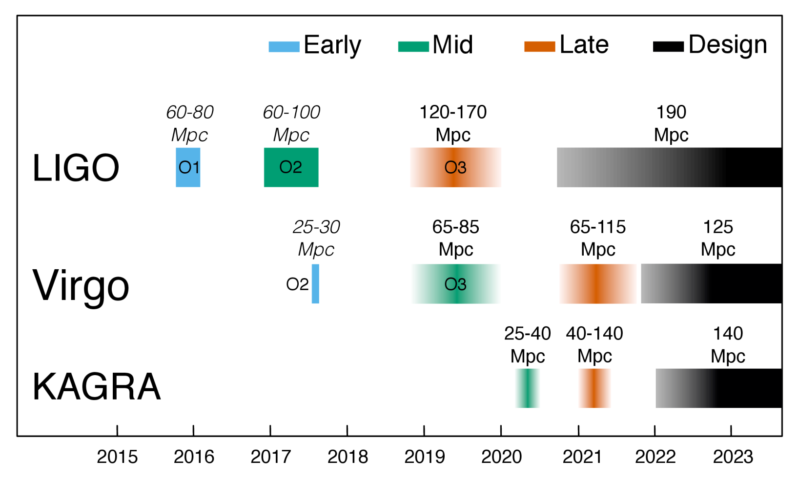
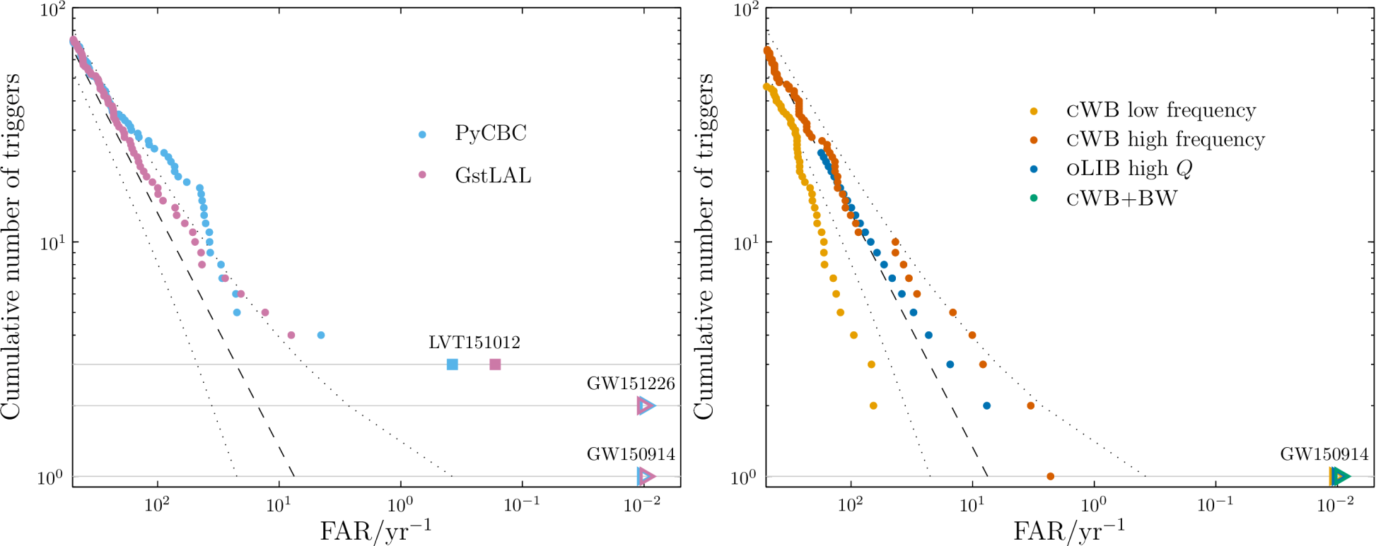
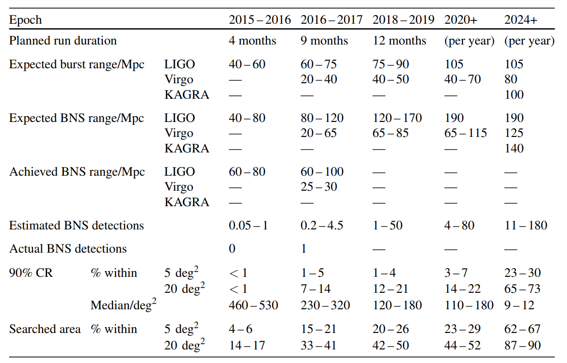


 ). The lower panel shows how we removed the glitch: the grey line shows


 is the component of the spin aligned with the orbital angular momentum. The two-dimensional shows the 90% probability contour, which follows a line of constant chirp mass. The one-dimensional plot shows individual masses; the dotted lines mark 90% bounds away from equal mass. Figure 4 of the
  .
.
 inferred from GW170817. The lines mark 68% and 95% intervals. The coloured bands are measurements from the cosmic microwave background (
 (assuming a uniform of neutron star masses between one and two solar masses). This is surprisingly close to what the Collaboration expected back in
  and
and  , with a realistic rate of
  . This means that we are on track to see many more binary neutron stars—perhaps one a week at design sensitivity!
 and spin
  of the final black hole. We could use other sets of parameters, but this pair compactly sum up the
  and
and  , if general relativity is a good match to the observations, then we expect everything to match up, and
 , indicated by the cross (+). The left panels show a general relativity simulation, and the right panel shows a waveform from a modified theory of gravity. Figure 1 of
  rather than


 (a much beloved combination of the two component masses which we are usually able to pin down precisely) and the total mass
  .
.
 is the mass of the stellar-mass black hole divided by the mass of the intermediate-mass black hole. Figure 1 of

 ). Figure 7 of


