On 4 January 2017, Advanced LIGO made a new detection of gravitational waves. The signal, which we call GW170104 [bonus note], came from the coalescence of two black holes, which inspiralled together (making that characteristic chirp) and then merged to form a single black hole.
On 4 January 2017, I was just getting up off the sofa when my phone buzzed. My new year’s resolution was to go for a walk every day, and I wanted to make use of the little available sunlight. However, my phone informed me that PyCBC (one or our search algorithms for signals from coalescing binaries) had identified an interesting event. I sat back down. I was on the rota to analyse interesting signals to infer their properties, and I was pretty sure that people would be eager to see results. They were. I didn’t leave the sofa for the rest of the day, bringing my new year’s resolution to a premature end.
Since 4 January, my time has been dominated by working on GW170104 (you might have noticed a lack of blog posts). Below I’ll share some of my war stories from life on the front line of gravitational-wave astronomy, and then go through some of the science we’ve learnt. (Feel free to skip straight to the science, recounting the story was more therapy for me).

Time–frequency plots for GW170104 as measured by Hanford (top) and Livingston (bottom). The signal is clearly visible as the upward sweeping chirp. The loudest frequency is something between E3 and G♯3 on a piano, and it tails off somewhere between D♯4/E♭4 and F♯4/G♭4. Part of Fig. 1 of the GW170104 Discovery Paper.
The story
In the second observing run, the Parameter Estimation group have divided up responsibility for analysing signals into two week shifts. For each rota shift, there is an expert and a rookie. I had assumed that the first slot of 2017 would be a quiet time. The detectors were offline over the holidays, due back online on 4 January, but the instrumentalists would probably find some extra tinkering they’d want to do, so it’d probably slip a day, and then the weather would be bad, so we’d probably not collect much data anyway… I was wrong. Very wrong. The detectors came back online on time, and there was a beautifully clean detection on day one.
My partner for the rota was Aaron Zimmerman. 4 January was his first day running parameter estimation on live signals. I think I would’ve run and hidden underneath my duvet in his case (I almost did anyway, and I lived through the madness of our first detection GW150914), but he rose to the occasion. We had first results after just a few hours, and managed to send out a preliminary sky localization to our astronomer partners on 6 January. I think this was especially impressive as there were some difficulties with the initial calibration of the data. This isn’t a problem for the detection pipelines, but does impact the parameters which we infer, particularly the sky location. The Calibration group worked quickly, and produced two updates to the calibration. We therefore had three different sets of results (one per calibration) by 6 January [bonus note]!
Producing the final results for the paper was slightly more relaxed. Aaron and I conscripted volunteers to help run all the various permutations of the analysis we wanted to double-check our results [bonus note].

Recovered gravitational waveforms from analysis of GW170104. The broader orange band shows our estimate for the waveform without assuming a particular source (wavelet). The narrow blue bands show results if we assume it is a binary black hole (BBH) as predicted by general relativity. The two match nicely, showing no evidence for any extra features not included in the binary black hole models. Figure 4 of the GW170104 Discovery Paper.
I started working on GW170104 through my parameter estimation duties, and continued with paper writing.
Ahead of the second observing run, we decided to assemble a team to rapidly write up any interesting binary detections, and I was recruited for this (I think partially because I’m not too bad at writing and partially because I was in the office next to John Veitch, one of the chairs of the Compact Binary Coalescence group,so he can come and check that I wasn’t just goofing off eating doughnuts). We soon decided that we should write a paper about GW170104, and you can decide whether or not we succeeded in doing this rapidly…
Being on the paper writing team has given me huge respect for the teams who led the GW150914 and GW151226 papers. It is undoubtedly one of the most difficult things I’ve ever done. It is extremely hard to absorb negative remarks about your work continuously for months [bonus note]—of course people don’t normally send comments about things that they like, but that doesn’t cheer you up when you’re staring at an inbox full of problems that need fixing. Getting a collaboration of 1000 people to agree on a paper is like herding cats while being a small duckling.
On of the first challenges for the paper writing team was deciding what was interesting about GW170104. It was another binary black hole coalescence—aren’t people getting bored of them by now? The signal was quieter than GW150914, so it wasn’t as remarkable. However, its properties were broadly similar. It was suggested that perhaps we should title the paper “GW170104: The most boring gravitational-wave detection”.
One potentially interesting aspect was that GW170104 probably comes from greater distance than GW150914 or GW151226 (but perhaps not LVT151012) [bonus note]. This might make it a good candidate for testing for dispersion of gravitational waves.
Dispersion occurs when different frequencies of gravitational waves travel at different speeds. A similar thing happens for light when travelling through some materials, which leads to prisms splitting light into a spectrum (and hence the creation of Pink Floyd album covers). Gravitational waves don’t suffered dispersion in general relativity, but do in some modified theories of gravity.
It should be easier to spot dispersion in signals which have travelled a greater distance, as the different frequencies have had more time to separate out. Hence, GW170104 looks pretty exciting. However, being further away also makes the signal quieter, and so there is more uncertainty in measurements and it is more difficult to tell if there is any dispersion. Dispersion is also easier to spot if you have a larger spread of frequencies, as then there can be more spreading between the highest and lowest frequencies. When you throw distance, loudness and frequency range into the mix, GW170104 doesn’t always come out on top, depending upon the particular model for dispersion: sometimes GW150914’s loudness wins, other times GW151226’s broader frequency range wins. GW170104 isn’t too special here either.
Even though GW170104 didn’t look too exciting, we started work on a paper, thinking that we would just have a short letter describing our observations. The Compact Binary Coalescence group decided that we only wanted a single paper, and we wouldn’t bother with companion papers as we did for GW150914. As we started work, and dug further into our results, we realised that actually there was rather a lot that we could say.
I guess the moral of the story is that even though you might be overshadowed by the achievements of your siblings, it doesn’t mean that you’re not awesome. There might not be one outstanding feature of GW170104, but there are lots of little things that make it interesting. We are still at the beginning of understanding the properties of binary black holes, and each new detection adds a little more to our picture.
I think GW170104 is rather neat, and I hope you do too.
As we delved into the details of our results, we realised there was actually a lot of things that we could say about GW170104, especially when considered with our previous observations. We ended up having to move some of the technical details and results to Supplemental Material. With hindsight, perhaps it would have been better to have a companion paper or two. However, I rather like how packed with science this paper is.
The paper, which Physical Review Letters have kindly accommodated, despite its length, might not be as polished a classic as the GW150914 Discovery Paper, but I think they are trying to do different things. I rarely ever refer to the GW150914 Discovery Paper for results (more commonly I use it for references), whereas I think I’ll open up the GW170104 Discovery Paper frequently to look up numbers.
Although perhaps not right away, I’d quite like some time off first. The weather’s much better now, perfect for walking…

Success! The view across Lac d’Annecy. Taken on a stroll after the Gravitational Wave Physics and Astronomy Workshop, the weekend following the publication of the paper.
The science
Advanced LIGO’s first observing run was hugely successful. Running from 12 September 2015 until 19 January 2016, there were two clear gravitational-wave detections, GW1501914 and GW151226, as well as a less certain candidate signal LVT151012. All three (assuming that they are astrophysical signals) correspond to the coalescence of binary black holes.
The second observing run started 30 November 2016. Following the first observing run’s detections, we expected more binary black hole detections. On 4 January, after we had collected almost 6 days’ worth of coincident data from the two LIGO instruments [bonus note], there was a detection.
The searches
The signal was first spotted by an online analysis. Our offline analysis of the data (using refined calibration and extra information about data quality) showed that the signal, GW170104, is highly significant. For both GstLAL and PyCBC, search algorithms which use templates to search for binary signals, the false alarm rate is estimated to be about 1 per 70,000 years.
The signal is also found in unmodelled (burst) searches, which look for generic, short gravitational wave signals. Since these are looking for more general signals than just binary coalescences, the significance associated with GW170104 isn’t as great, and coherent WaveBurst estimates a false alarm rate of 1 per 20,000 years. This is still pretty good! Reconstructions of the waveform from unmodelled analyses also match the form expected for binary black hole signals.
The search false alarm rates are the rate at which you’d expect something this signal-like (or more signal-like) due to random chance, if you data only contained noise and no signals. Using our knowledge of the search pipelines, and folding in some assumptions about the properties of binary black holes, we can calculate a probability that GW170104 is a real astrophysical signal. This comes out to be greater than 
The source
As for the previous gravitational wave detections, GW170104 comes from a binary black hole coalescence. The initial black holes were 


Estimated masses for the two black holes in the binary 
GW150914 was the first time that we had observed stellar-mass black holes with masses greater than around 
Black holes have two important properties: mass and spin. We have good measurements on the masses of the two initial black holes, but not the spins. The sensitivity of the form of the gravitational wave to spins can be described by two effective spin parameters, which are mass-weighted combinations of the individual spins.
- The effective inspiral spin parameter
qualifies the impact of the spins on the rate of inspiral, and where the binary plunges together to merge. It ranges from +1, meaning both black holes are spinning as fast as possible and rotate in the same direction as the orbital motion, to −1, both black holes spinning as fast as possible but in the opposite direction to the way that the binary is orbiting. A value of 0 for
- The effective precession spin parameter
qualifies the amount of precession, the way that the orbital plane and black hole spins wobble when they are not aligned. It is 0 for no precession, and 1 for maximal precession.
We can place some constraints on 


Estimated effective inspiral spin parameter
Converting the information about

Estimated orientation and magnitude of the two component spins. The distribution for the more massive black hole is on the left, and for the smaller black hole on the right. The probability is binned into areas which have uniform prior probabilities, so if we had learnt nothing, the plot would be uniform. Part of Figure 3 of the GW170104 Discovery Paper.
One of the comments we had on a draft of the paper was that we weren’t making any definite statements about the spins—we would have if we could, but we can’t for GW170104, at least for the spins of the two inspiralling black holes. We can be more definite about the spin of the final black hole. If two similar mass black holes spiral together, the angular momentum from the orbit is enough to give a spin of around 


Estimated mass 

If you’re interested in parameter describing GW170104, make sure to check out the big table in the Supplemental Material. I am a fan of tables [bonus note].
Merger rates
Adding the first 11 days of coincident data from the second observing run (including the detection of GW170104) to the results from the first observing run, we find merger rates consistent with those from the first observing run.
To calculate the merger rates, we need to assume a distribution of black hole masses, and we use two simple models. One uses a power law distribution for the primary (larger) black hole and a uniform distribution for the mass ratio; the other uses a distribution uniform in the logarithm of the masses (both primary and secondary). The true distribution should lie somewhere between the two. The power law rate density has been updated from 


Astrophysics
The discoveries from the first observing run showed that binary black holes exist and merge. The question is now how exactly they form? There are several suggested channels, and it could be there is actually a mixture of different formation mechanisms in action. It will probably require a large number of detections before we can make confident statements about the the probable formation mechanisms; GW170104 is another step towards that goal.
There are two main predicted channels of binary formation:
- Isolated binary evolution, where a binary star system lives its life together with both stars collapsing to black holes at the end. To get the black holes close enough to merge, it is usually assumed that the stars go through a common envelope phase, where one star puffs up so that the gravity of its companion can steal enough material that they lie in a shared envelope. The drag from orbiting inside this then shrinks the orbit.
- Dynamical evolution where black holes form in dense clusters and a binary is created by dynamical interactions between black holes (or stars) which get close enough to each other.
It’s a little artificial to separate the two, as there’s not really such a thing as an isolated binary: most stars form in clusters, even if they’re not particularly large. There are a variety of different modifications to the two main channels, such as having a third companion which drives the inner binary to merge, embedding the binary is a dense disc (as found in galactic centres), or dynamically assembling primordial black holes (formed by density perturbations in the early universe) instead of black holes formed through stellar collapse.
All the channels can predict black holes around the masses of GW170104 (which is not surprising given that they are similar to the masses of GW150914).
The updated rates are broadly consistent with most channels too. The tightening of the uncertainty of the rates means that the lower bound is now a little higher. This means some of the channels are now in tension with the inferred rates. Some of the more exotic channels—requiring a third companion (Silsbee & Tremain 2017; Antonini, Toonen & Hamers 2017) or embedded in a dense disc (Bartos et al. 2016; Stone, Metzger & Haiman 2016; Antonini & Rasio 2016)—can’t explain the full rate, but I don’t think it was ever expected that they could, they are bonus formation mechanisms. However, some of the dynamical models are also now looking like they could predict a rate that is a bit low (Rodriguez et al. 2016; Mapelli 2016; Askar et al. 2017; Park et al. 2017). Assuming that this result holds, I think this may mean that some of the model parameters need tweaking (there are more optimistic predictions for the merger rates from clusters which are still perfectly consistent), that this channel doesn’t contribute all the merging binaries, or both.
The spins might help us understand formation mechanisms. Traditionally, it has been assumed that isolated binary evolution gives spins aligned with the orbital angular momentum. The progenitor stars were probably more or less aligned with the orbital angular momentum, and tides, mass transfer and drag from the common envelope would serve to realign spins if they became misaligned. Rodriguez et al. (2016) gives a great discussion of this. Dynamically formed binaries have no correlation between spin directions, and so we would expect an isotropic distribution of spins. Hence it sounds quite simple: misaligned spins indicates dynamical formation (although we can’t tell if the black holes are primordial or stellar), and aligned spins indicates isolated binary evolution. The difficulty is the traditional assumption for isolated binary evolution potentially ignores a number of effects which could be important. When a star collapses down to a black hole, there may be a supernova explosion. There is an explosion of matter and neutrinos and these can give the black hole a kick. The kick could change the orbital plane, and so misalign the spin. Even if the kick is not that big, if it is off-centre, it could torque the black hole, causing it to rotate and so misalign the spin that way. There is some evidence that this can happen with neutron stars, as one of the pulsars in the double pulsar system shows signs of this. There could also be some instability that changes the angular momentum during the collapse of the star, possibly with different layers rotating in different ways [bonus note]. The spin of the black hole would then depend on how many layers get swallowed. This is an area of research that needs to be investigated further, and I hope the prospect of gravitational wave measurements spurs this on.
For GW170104, we know the spins are not large and aligned with the orbital angular momentum. This might argue against one variation of isolated binary evolution, chemically homogeneous evolution, where the progenitor stars are tidally locked (and so rotate aligned with the orbital angular momentum and each other). Since the stars are rapidly spinning and aligned, you would expect the final black holes to be too, if the stars completely collapse down as is usually assumed. If the stars don’t completely collapse down though, it might still be possible that GW170104 fits with this model. Aside from this, GW170104 is consistent with all the other channels.

Estimated effective inspiral spin parameter 
If we start looking at the population of events, we do start to notice something about the spins. All of the inferred values of
Tests of general relativity
As well as giving us an insight into the properties of black holes, gravitational waves are the perfect tools for testing general relativity. If there are any corrections to general relativity, you’d expect them to be most noticeable under the most extreme conditions, where gravity is strong and spacetime is rapidly changing, exactly as in a binary black hole coalescence.
For GW170104 we repeated tests previously performed. Again, we found no evidence of deviations.
We added extra terms to to the waveform and constrained their potential magnitudes. The results are pretty much identical to at the end of the first observing run (consistent with zero and hence general relativity). GW170104 doesn’t add much extra information, as GW150914 typically gives the best constraints on terms that modify the post-inspiral part of the waveform (as it is louder), while GW151226 gives the best constraint on the terms which modify the inspiral (as it has the longest inspiral).
We also chopped the waveform at a frequency around that of the innermost stable orbit of the remnant black hole, which is about where the transition from inspiral to merger and ringdown occurs, to check if the low frequency and high frequency portions of the waveform give consistent estimates for the final mass and spin. They do.
We have also done something slightly new, and tested for dispersion of gravitational waves. We did something similar for GW150914 by putting a limit on the mass of the graviton. Giving the graviton mass is one way of adding dispersion, but we consider other possible forms too. In all cases, results are consistent with there being no dispersion. While we haven’t discovered anything new, we can update our gravitational wave constraint on the graviton mass of less than 
The search for counterparts
We don’t discuss observations made by our astronomer partners in the paper (they are not our results). A number (28 at the time of submission) of observations were made, and I expect that there will be a series of papers detailing these coming soon. So far papers have appeared from:
- AGILE—hard X-ray and gamma-ray follow-up. They didn’t find any gamma-ray signals, but did identify a weak potential X-ray signal occurring about 0.46 s before GW170104. It’s a little odd to have a signal this long before the merger. The team calculate a probability for such a coincident to happen by chance, and find quite a small probability, so it might be interesting to follow this up more (see the INTEGRAL results below), but it’s probably just a coincidence (especially considering how many people did follow-up the event).
- ANTARES—a search for high-energy muon neutrinos. No counterparts are identified in a ±500 s window around GW170104, or over a ±3 month period.
- AstroSat-CZTI and GROWTH—a collaboration of observations across a range of wavelengths. They don’t find any hard X-ray counterparts. They do follow up on a bright optical transient ATLASaeu, suggested as a counterpart to GW170104, and conclude that this is a likely counterpart of long, soft gamma-ray burst GRB 170105A.
- ATLAS and Pan-STARRS—optical follow-up. They identified a bright optical transient 23 hours after GW170104, ATLAS17aeu. This could be a counterpart to GRB 170105A. It seems unlikely that there is any mechanism that could allow for a day’s delay between the gravitational wave emission and an electromagnetic signal. However, the team calculate a small probability (few percent) of finding such a coincidence in sky position and time, so perhaps it is worth pondering. I wouldn’t put any money on it without a distance estimate for the source: assuming it’s a normal afterglow to a gamma-ray burst, you’d expect it to be further away than GW170104’s source.
- Borexino—a search for low-energy neutrinos. This paper also discusses GW150914 and GW151226. In all cases, the observed rate of neutrinos is consistent with the expected background.
- CALET—a gamma-ray search. This paper includes upper limits for GW151226, GW170104, GW170608, GW170814 and GW170817.
- DLT40—an optical search designed for supernovae. This paper covers the whole of O2 including GW170608, GW170814, GW170817 plus GW170809 and GW170823.
- Fermi (GBM and LAT)—gamma-ray follow-up. They covered an impressive fraction of the sky localization, but didn’t find anything.
- INTEGRAL—gamma-ray and hard X-ray observations. No significant emission is found, which makes the event reported by AGILE unlikely to be a counterpart to GW170104, although they cannot completely rule it out.
- The intermediate Palomar Transient Factory—an optical survey. While searching, they discovered iPTF17cw, a broad-line type Ic supernova which is unrelated to GW170104 but interesting as it an unusual find.
- Mini-GWAC—a optical survey (the precursor to GWAC). This paper covers the whole of their O2 follow-up including GW170608.
- NOvA—a search for neutrinos and cosmic rays over a wide range of energies. This paper covers all the events from O1 and O2, plus triggers from O3.
- The Owens Valley Radio Observatory Long Wavelength Array—a search for prompt radio emission.
- TOROS—optical follow-up. They identified no counterparts to GW170104 (although they did for GW170817).
If you are interested in what has been reported so far (no compelling counterpart candidates yet to my knowledge), there is an archive of GCN Circulars sent about GW170104.
Summary
Advanced LIGO has made its first detection of the second observing run. This is a further binary black hole coalescence. GW170104 has taught us that:
- The discoveries of the first observing run were not a fluke. There really is a population of stellar mass black holes with masses above
- Binary black hole spins may be typically misaligned or small. This is not certain yet, but it is certainly worth investigating potential mechanisms that could cause misalignment.
- General relativity still works, even after considering our new tests.
- If someone asks you to write a discovery paper, run. Run and do not look back.
Title: GW170104: Observation of a 50-solar-mass binary black hole coalescence at redshift 0.2
Journal: Physical Review Letters; 118(22):221101(17); 2017 (Supplemental Material)
arXiv: 1706.01812 [gr-qc]
Data release: GRavitational Wave Open Science Center
Science summary: GW170104: Observation of a 50-solar-mass binary black hole coalescence at redshift 0.2
If you’re looking for the most up-to-date results regarding GW170104, check out the O2 Catalogue Paper.
Bonus notes
Naming
Gravitational wave signals (at least the short ones, which are all that we have so far), are named by their detection date. GW170104 was discovered 2017 January 4. This isn’t too catchy, but is at least better than the ID number in our database of triggers (G268556) which is used in corresponding with our astronomer partners before we work out if the “GW” title is justified.
Previous detections have attracted nicknames, but none has stuck for GW170104. Archisman Ghosh suggested the Perihelion Event, as it was detected a few hours before the Earth reached its annual point closest to the Sun. I like this name, its rather poetic.
More recently, Alex Nitz realised that we should have called GW170104 the Enterprise-D Event, as the USS Enterprise’s registry number was NCC-1701. For those who like Star Trek: the Next Generation, I hope you have fun discussing whether GW170104 is the third or fourth (counting LVT151012) detection: “There are four detections!“
The 6 January sky map
I would like to thank the wi-fi of Chiltern Railways for their role in producing the preliminary sky map. I had arranged to visit London for the weekend (because my rota slot was likely to be quiet… ), and was frantically working on the way down to check results so they could be sent out. I’d also like to thank John Veitch for putting together the final map while I was stuck on the Underground.
Binary black hole waveforms
The parameter estimation analysis works by matching a template waveform to the data to see how well it matches. The results are therefore sensitive to your waveform model, and whether they include all the relevant bits of physics.
In the first observing run, we always used two different families of waveforms, to see what impact potential errors in the waveforms could have. The results we presented in discovery papers used two quick-to-calculate waveforms. These include the effects of the black holes’ spins in different ways
- SEOBNRv2 has spins either aligned or antialigned with the orbital angular momentum. Therefore, there is no precession (wobbling of orientation, like that of a spinning top) of the system.
- IMRPhenomPv2 includes an approximate description of precession, packaging up the most important information about precession into a single parameter
For GW150914, we also performed a follow-up analysis using a much more expensive waveform SEOBNRv3 which more fully includes the effect of both spins on precession. These results weren’t ready at the time of the announcement, because the waveform is laborious to run.
For GW170104, there were discussions that using a spin-aligned waveform was old hat, and that we should really only use the two precessing models. Hence, we started on the endeavour of producing SEOBNRv3 results. Fortunately, the code has been sped up a little, although it is still not quick to run. I am extremely grateful to Scott Coughlin (one of the folks behind Gravity Spy), Andrea Taracchini and Stas Babak for taking charge of producing results in time for the paper, in what was a Herculean effort.
I spent a few sleepless nights, trying to calculate if the analysis was converging quickly enough to make our target submission deadline, but it did work out in the end. Still, don’t necessarily expect we’ll do this for a all future detections.
Since the waveforms have rather scary technical names, in the paper we refer to IMRPhenomPv2 as the effective precession model and SEOBNRv3 as the full precession model.
On distance
Distance measurements for gravitational wave sources have significant uncertainties. The distance is difficult to measure as it determined from the signal amplitude, but this is also influences by the binary’s inclination. A signal could either be close and edge on or far and face on-face off.

Estimated luminosity distance 

The uncertainty on the distance rather awkwardly means that we can’t definitely say that GW170104 came from a further source than GW150914 or GW151226, but it’s a reasonable bet. The 90% credible intervals on the distances are 250–570 Mpc for GW150194, 250–660 Mpc for GW151226, 490–1330 Mpc for GW170104 and 500–1500 Mpc for LVT151012.
Translating from a luminosity distance to a travel time (gravitational waves do travel at the speed of light, our tests of dispersion are consistent wit that!), the GW170104 black holes merged somewhere between 1.3 and 3.0 billion years ago. This is around the time that multicellular life first evolved on Earth, and means that black holes have been colliding longer than life on Earth has been reproducing sexually.
Time line
A first draft of the paper (version 2; version 1 was a copy-and-paste of the Boxing Day Discovery Paper) was circulated to the Compact Binary Coalescence and Burst groups for comments on 4 March. This was still a rough version, and we wanted to check that we had a good outline of the paper. The main feedback was that we should include more about the astrophysical side of things. I think the final paper has a better balance, possibly erring on the side of going into too much detail on some of the more subtle points (but I think that’s better than glossing over them).
A first proper draft (version 3) was released to the entire Collaboration on 12 March in the middle of our Collaboration meeting in Pasadena. We gave an oral presentation the next day (I doubt many people had read the paper by then). Collaboration papers are usually allowed two weeks for people to comment, and we followed the same procedure here. That was not a fun time, as there was a constant trickle of comments. I remember waking up each morning and trying to guess how many emails would be in my inbox–I normally low-balled this.
I wasn’t too happy with version 3, it was still rather rough. The members of the Paper Writing Team had been furiously working on our individual tasks, but hadn’t had time to look at the whole. I was much happier with the next draft (version 4). It took some work to get this together, following up on all the comments and trying to address concerns was a challenge. It was especially difficult as we got a series of private comments, and trying to find a consensus probably made us look like the bad guys on all sides. We released version 4 on 14 April for a week of comments.
The next step was approval by the LIGO and Virgo executive bodies on 24 April. We prepared version 5 for this. By this point, I had lost track of which sentences I had written, which I had merely typed, and which were from other people completely. There were a few minor changes, mostly adding technical caveats to keep everyone happy (although they do rather complicate the flow of the text).
The paper was circulated to the Collaboration for a final week of comments on 26 April. Most comments now were about typos and presentation. However, some people will continue to make the same comment every time, regardless of how many times you explain why you are doing something different. The end was in sight!
The paper was submitted to Physical Review Letters on 9 May. I was hoping that the referees would take a while, but the reports were waiting in my inbox on Monday morning.
The referee reports weren’t too bad. Referee A had some general comments, Referee B had some good and detailed comments on the astrophysics, and Referee C gave the paper a thorough reading and had some good suggestions for clarifying the text. By this point, I have been staring at the paper so long that some outside perspective was welcome. I was hoping that we’d have a more thorough review of the testing general relativity results, but we had Bob Wald as one of our Collaboration Paper reviewers (the analysis, results and paper are all reviewed internally), so I think we had already been held to a high standard, and there wasn’t much left to say.
We put together responses to the reports. There were surprisingly few comments from the Collaboration at this point. I guess that everyone was getting tired. The paper was resubmitted and accepted on 20 May.
One of the suggestions of Referee A was to include some plots showing the results of the searches. People weren’t too keen on showing these initially, but after much badgering they were convinced, and it was decided to put these plots in the Supplemental Material which wouldn’t delay the paper as long as we got the material submitted by 26 May. This seemed like plenty of time, but it turned out to be rather frantic at the end (although not due to the new plots). The video below is an accurate representation of us trying to submit the final version.
I have an email which contains the line “Many Bothans died to bring us this information” from 1 hour and 18 minutes before the final deadline.
After this, things were looking pretty good. We had returned the proofs of the main paper (I had a fun evening double checking the author list. Yes, all of them). We were now on version 11 of the paper.
Of course, there’s always one last thing. On 31 May, the evening before publication, Salvo Vitale spotted a typo. Nothing serious, but annoying. The team at Physical Review Letters were fantastic, and took care of it immediately!
There’ll still be one more typo, there always is…
Looking back, it is clear that the principal bottle-neck in publishing the results is getting the Collaboration to converge on the paper. I’m not sure how we can overcome this… Actually, I have some ideas, but none that wouldn’t involve some form of doomsday device.
Detector status
The sensitivities of the LIGO Hanford and Livinston detectors are around the same as they were in the first observing run. After the success of the first observing run, the second observing run is the difficult follow up album. Livingston has got a little better, while Hanford is a little worse. This is because the Livingston team concentrate on improving low frequency sensitivity whereas the Hanford team focused on improving high frequency sensitivity. The Hanford team increased the laser power, but this introduces some new complications. The instruments are extremely complicated machines, and improving sensitivity is hard work.
The current plan is to have a long commissioning break after the end of this run. The low frequency tweaks from Livingston will be transferred to Hanford, and both sites will work on bringing down other sources of noise.
While the sensitivity hasn’t improved as much as we might have hoped, the calibration of the detectors has! In the first observing run, the calibration uncertainty for the first set of published results was about 10% in amplitude and 10 degrees in phase. Now, uncertainty is better than 5% in amplitude and 3 degrees in phase, and people are discussing getting this down further.
Spin evolution
As the binary inspirals, the orientation of the spins will evolve as they precess about. We always quote measurements of the spins at a point in the inspiral corresponding to a gravitational wave frequency of 20 Hz. This is most convenient for our analysis, but you can calculate the spins at other points. However, the resulting probability distributions are pretty similar at other frequencies. This is because the probability distributions are primarily determined by the combination of three things: (i) our prior assumption of a uniform distribution of spin orientations, (ii) our measurement of the effective inspiral spin, and (iii) our measurement of the mass ratio. A uniform distribution stays uniform as spins evolve, so this is unaffected, the effective inspiral spin is approximately conserved during inspiral, so this doesn’t change much, and the mass ratio is constant. The overall picture is therefore qualitatively similar at different moments during the inspiral.
Footnotes
I love footnotes. It was challenging for me to resist having any in the paper.
Gravity waves
It is possible that internal gravity waves (that is oscillations of the material making up the star, where the restoring force is gravity, not gravitational waves, which are ripples in spacetime), can transport angular momentum from the core of a star to its outer envelope, meaning that the two could rotate in different directions (Rogers, Lin & Lau 2012). I don’t think anyone has studied this yet for the progenitors of binary black holes, but it would be really cool if gravity waves set the properties of gravitational wave sources.
I really don’t want to proof read the paper which explains this though.
Colour scheme
For our plots, we use a consistent colour coding for our events. GW150914 is blue; LVT151012 is green; GW151226 is red–orange, and GW170104 is purple. The colour scheme is designed to be colour blind friendly (although adopting different line styles would perhaps be more distinguishable), and is implemented in Python in the Seaborn package as colorblind. Katerina Chatziioannou, who made most of the plots showing parameter estimation results is not a fan of the colour combinations, but put a lot of patient effort into polishing up the plots anyway.
 ,
, and
and  are the masses of the two components of the binary. By looking at the signal (go on, try the
  at different times, and so track how it changes. You can rewrite the equation for the rate of change of the gravitational wave frequency
  , to give an expression for the chirp mass
 .
. and
and  are the speed of light and the gravitational constant, which usually pop up in general relativity equations. If you use this formula (perhaps fitting for the trend
  [
[ . The orbital frequency is half this, so
  . The orbital separation
  is related to the frequency by
![\displaystyle R = \left[\frac{GM}{(2\pi f_\mathrm{orb})^2}\right]^{1/3}](https://s0.wp.com/latex.php?latex=%5Cdisplaystyle+R+%3D+%5Cleft%5B%5Cfrac%7BGM%7D%7B%282%5Cpi+f_%5Cmathrm%7Borb%7D%29%5E2%7D%5Cright%5D%5E%7B1%2F3%7D&bg=ffffff&fg=444444&s=0&c=20201002) ,
, is the binary’s total mass. This formula is only strictly true in
  . We now want to compare the binary’s separation to the size of black hole with the same mass. A
  .
. . A compactness of
  could only happen for black holes. We could maybe get a binary made of two neutron stars to have a compactness of
  , but the system is too heavy to contain two neutron stars (which have a maximum mass of about
  ). The system is so compact, it must contain black holes!
 , the lighter black hole
  and the final black hole (resulting from the coalescence)

 means the binary is face on,
  means it face off, and an inclination around
  is edge on. The bands show the recovered 90% credible interval; the dark lines the median values, and the dotted lines show the true values. The (grey) polarization angle
  was chosen so that the detectors are approximately insensitive to the
  polarization. Figure 4 of the
  and ignores earlier cycles. The standard analysis includes data down to
  , and this extra data does give you a little information about precession. (The limit of the simulation length also means you shouldn’t expect this type of analysis for the longer LVT151012 or GW151226 any time soon).
![\displaystyle L \propto \exp \left[- \int_{-\infty}^{\infty} \mathrm{d}f \frac{|s(f) - h(f)|^2}{S_n(f)} \right]](https://s0.wp.com/latex.php?latex=%5Cdisplaystyle+L+%5Cpropto+%5Cexp+%5Cleft%5B-+%5Cint_%7B-%5Cinfty%7D%5E%7B%5Cinfty%7D+%C2%A0%5Cmathrm%7Bd%7Df+%C2%A0%5Cfrac%7B%7Cs%28f%29+-+h%28f%29%7C%5E2%7D%7BS_n%28f%29%7D+%C2%A0%5Cright%5D&bg=ffffff&fg=444444&s=0&c=20201002) ,
, is the signal,
  is our waveform template and
  is the noise spectral density (
 is accurate. I think that the denominator
  . You need proper templates for the gravitational wave signal to calculate this. If you factor in the the gravitational wave gets redshifted (shifted to lower frequency by the expansion of the Universe), then the true chirp mass of the source system is
  .
. —the total mass of the binary,
  —the chirp mass, the combination of the two component masses which sets how the binary inspirals together;
 —the mass ratio,
  . Confusingly, numerical relativists often use the opposite convention
  (which is why the
  : we can keep the standard definition, but all the numbers are numerical relativist friendly).
 , where
  is the true, redshift-corrected source-frame mass and
  is the redshift. The mass ratio
  would be now);
 —the inclination, the angle between the line of sight and the orbital angular momentum (
 ). This is zero for a face-on binary.
 ) and the total angular momentum of the binary (
 ); this is approximately equal to the inclination, but is easier to use for precessing binaries.
 (no spin) and
  (maximum spin);
 —the primary tilt angle, the angle between the orbital angular momentum and the heavier black holes spin (
 ). This is zero for aligned spin.
 —the secondary tilt angle, the angle between the orbital angular momentum and the lighter black holes spin (
 ).
). —the angle between the projections of the two spins on the orbital plane.
 —the polarization angle, this is zero when the detector arms are parallel to the
 , the mass ratio
  and the total mass


 and
and  , which are pretty good!
 and
and  [
[ is the mass of our Sun (about 330,000 times the mass of the Earth). The error bars indicate our
 is defined to be bigger than
  . Figure 3 of
  [
[ of energy (where

 for PyCBC, and a ratio of likelihood for the signal and noise hypotheses
  for GstLAL). A larger detection statistic means something is more signal-like and we assess the significance by comparing with the background of noise events. The further above the background curve an event is, the more significant it is. We have three events that stand out.
 . Part of Figure 4 of the
  and the effective spin parameter

 and spins


 in the Testing General Relativity Paper) are parameters that affect the inspiral. The final box on the right is for parameters which impact the merger and ringdown. The top row shows results for GW150914, these are updated results using the improved calibrated data. The second row shows results for GW151226, and the bottom row shows what happens when you combine the two.
 parameters.
 , which we expect gives a sensible upper bound on the rate.
 , 2.
, 2.  , and 3.
 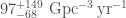 . As expected, the first rate is nestled between the other two.
 , and that the less massive black hole has a mass uniformly distributed in mass ratio, down to a minimum black hole mass of
  . The cut-off, is the edge of a speculated
  . This has significant uncertainty, so we can’t say too much yet. This is a slightly steeper slope than used for the power-law rate (although entirely consistent with it), which would nudge the rates a little lower. The slope does fit in with fits to the distribution of masses in X-ray binaries. I’m excited to see how O2 will change our understanding of the distribution.
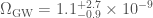 at a frequency of 25 Hz to
 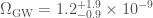 . This might be measurable after a few years at design sensitivity.
 . Therefore we still have to do the same about searches for anything else. The results from searches for other compact binaries should appear soon (
 . The median should really round to
  as to three significant figures it is
  . This really confused everyone though, as with rounding you’d have a binary with components of masses
  and
and  . Rounding is a pain! Fortunately,
  .
.
 .
.


 ). Figure 7 of
 , the plan is to go up to
  . This will reduce shot noise, but raises all sorts of control issues, such as how to avoid
 : the probability of finding the particular values of the signal-to-noise ratio and residual in both detectors for signals (assuming signal sources are uniformly distributed isotropically in space), divided by the probability of finding them for noise.
 and for some reason we’ve copied them. The second most significant event (around
  ) is LVT151012. Fig. 7 from the
  . GstLAL calculates a false alarm probability of
  , but this is reaching the level that we have to worry about the accuracy of assumptions that go into this (that the distribution of noise triggers in uniform across templates—if this is not the case, the false alarm probability could be about
  times larger). Therefore, for our overall result, we stick to the upper bound, which is consistent with both searches. The false alarm probability is so tiny, I don’t think anyone doubts this signal is real.
 , compared with GW150914’s
  , so it is quiet. The false alarm probability from PyCBC is
  , and from GstLAL is
  , consistent with what we would expect for such a signal. LVT151012 does not reach the standards we would like to claim a detection, but it is still interesting.
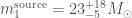 and
and  (the asymmetric uncertainties come from imposing
  . The effective spin, as for GW150914, is close to zero
  . The luminosity distance is
  , meaning it is about twice as far away as GW150914’s source. I hope we’ll write more about this event in the future; there are some more details in the


 means we are looking at the binary (approximately) edge-on. Results are shown for the EOBNR waveform and the IMRPhenom: both agree well. The Overall results come from averaging the two. The dotted lines mark the edge of our 90% probability intervals. Fig. 2 from the
 : the
: the  parameters cover the intermediate regime. If the deviation
  is zero, the value coincides with the value from general relativity. The plot shows what would happen if you allow all the variable to vary at once (the multiple results) and if you tried just that parameter on its own (the single results).
 ,
,  and
and  all show this behaviour, as they are sensitive to similar noise features. These measurements are much tighter than from any test we’ve done before, except for the measurement of
  which is better measured from the
  ; 2.
; 2. 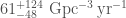 , and 3.
 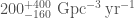 . There is a huge scatter, but the flat and power-law rates hopefully bound the true value.
 more detections. This is shown in the plot below. It looks like there’s about about a 10% chance of not seeing anything else in O1, but we’re confident that we’ll have 10 more by the end of O2, and 35 more by the end of O3! I may need to lie down…
 is something like a signal-to-noise ratio constructed based upon the correlated power in the detectors. The value for GW150914 was
  , which is higher than for any other candidate. The false alarm probability (or p-value), folding in all three search classes, is
  , which is pretty tiny, even if not as significant as for the tailored compact binary searches.
 (which agrees with the cWB estimate if you only consider chirp-like triggers).
 . Fig. 6 of the
  for earthquakes, although it can be higher if the epicentre is near), unless there is motion in the optics around (which can couple to cause higher frequency noise). There is a network of seismometers to measure earthquakes at both sites. There where two magnitude 2.1
  and
and  is done to monitor and control several parts of the optics. There is a fault somewhere in the system which means that there is a coupling to the output channel and we get noise across
  to
to  , which is where we look for compact binary coalescences. Rai Weiss suggested
  ) to be confused with binary black holes, but don’t have the right frequency evolution. They contribute to the background of noise triggers in the
 ) lightning strike in the same second as GW150914 over Burkino Faso. However, the magnetic disturbances were at least a thousand times too small to explain the amplitude of GW150914.
 . The significance of GW150914 is so great that we don’t really need to worry about the effects of vetoes.

 is changed into the measured strain
  is shown below. The calibration pipeline build models to correct for the effects of the control system to provide an accurate model of the true gravitational wave strain.
 is converted into the measured signal
  between
  , and the uncertainty in phase calibration is less than
  . These are the values that we use in our
 and the 90% area is
  . However, including calibration uncertainty, the sky areas are
  at 50% and 90% probability respectively. Calibration uncertainty has the largest effect on sky area. All the sky maps agree that the source is in in some region of the annulus set by the time delay between the two detectors.
 between the two detectors. BAYESTAR rapidly computes sky maps for binary coalescences, but it needs the output of one of the detection pipelines to run, and so was not available at low latency. The

 without also worrying about the distribution of parameters like the black hole masses. The signal-to-noise ratio is inversely proportional to distance, and we expect sources to be uniformly distributed in volume. Putting these together (and ignoring corrections from cosmology) gives a distribution for signal-to-noise ratio of
  (
(


 and
and  , where
  kilograms). If you’re curious what’s going with these numbers and the pluses and minuses, check out this
  , and the small one has spin
  (these numbers have been rounded). These aren’t great measurements. For the smaller black hole, its spin is almost equally probable to take any allowed value; this isn’t quite the case, but we haven’t learnt much about its size. For the bigger black hole, we do slightly better, and it seems that the spin is on the smaller side. This is interesting, as measurements of spins for black holes in X-ray binaries tend to be on the higher side: perhaps there are different types of black holes?
 . This could mean that both black holes have small spins, or that they have larger spins that aren’t aligned with the orbit (or each other). We have learnt something about the spins, it’s just not too easy to tease that apart to give values for each of the black holes.
 . It is the new record holder for the largest observed stellar-mass black hole!
 of energy was radiated away as gravitational waves (where
  , which is in the middling-to-high range. You’ll notice that we can deduce this to a much higher precisely than the spins of the two initial black holes. This is because it is largely fixed by the orbital angular momentum of the binary, and so its value is set by orbital dynamics and gravitational physics. I think its incredibly satisfying that we we can such a clean measurement of the spin.
 for the final black hole. The dotted lines mark the edge of our 90% probability intervals. The different coloured curves show different models: they agree which still makes me incredibly happy! Fig. 3 from the
  (about six times the length of the
  (about five and a half M25s, so maybe this would be the better route for your morning commute). The total area of the event horizon is about
  . If you flattened this out, it would cover an area about the size of Montana.
  , a megaparsec is a unit of length (regardless of what Han Solo thinks) equal to about 3 million light-years. The luminosity distance isn’t quite the same as the distance you would record using a tape measure because it takes into account the effects of the expansion of the Universe. But it’s pretty close. Using our 90% probability range, the merger would have happened sometime between 700 million years and 1.6 billion years ago. This coincides with the
  of the sky. For comparison, the full Moon is about
  . This is a large area to cover with a telescope, and we don’t expect there to be anything to see for a black hole merger, but that hasn’t stopped our intrepid partners from trying. For a lovely visualisation of where we think the source could be, marvel at the
  (in units that the particle physicists like). This is tiny! It is about as many times lighter than an electron as an electron is lighter than a teaspoon of water (well,
  , which is just under a full teaspoon), or as many times lighter than the almost teaspoon of water is than three Earths.
 of the graviton from The Event (GW150914). The
 , we think there’s a 5% chance that the mass is below
 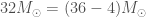 , and a 5% chance it’s above
  , so we write our result as


