Advanced LIGO and Advanced Virgo have detected their first binary neutron star inspiral. Remarkably, this event was observed not just with gravitational waves, but also across the electromagnetic spectrum, from gamma-rays to radio. This discovery confirms the theory that binary neutron star mergers are the progenitors of short gamma-ray bursts and kilonovae, and may be the primary source of heavy elements like gold.
In this post, I’ll go through some of the story of GW170817. As for GW150914, I’ll write another post on the more technical details of our papers, once I’ve had time to catch up on sleep.
Discovery
The second observing run (O2) of the advanced gravitational-wave detectors started on 30 November 2016. The first detection came in January—GW170104. I was heavily involved in the analysis and paper writing for this. We finally finished up in June, at which point I was thoroughly exhausted. I took some time off in July [bonus note], and was back at work for August. With just one month left in the observing run, it would all be downhill from here, right?
August turned out to be the lava-filled, super-difficult final level of O2. As we have now announced, on August 14, we detected a binary black hole coalescence—GW170814. This was the first clear detection including Virgo, giving us superb sky localization. This is fantastic for astronomers searching for electromagnetic counterparts to our gravitational-wave signals. There was a flurry of excitement, and we thought that this was a fantastic conclusion to O2. We were wrong, this was just the save point before the final opponent. On August 17, we met the final, fire-ball throwing boss.
Text messages from our gravitational-wave candidate event database GraceDB. The final message is for GW170817, or as it was known at the time, G298048. It certainly caught my attention. The messages above are for GW170814, that was picked up multiple times by our search algorithms. It was a busy week.
At 1:58 pm BST my phone buzzed with a text message, an automated alert of a gravitational-wave trigger. I was obviously excited—I recall that my exact thoughts were “What fresh hell is this?” I checked our online event database and saw that it was a single-detector trigger, it was only seen by our Hanford instrument. I started to relax, this was probably going to turn out to be a glitch. The template masses, were low, in the neutron star range, not like the black holes we’ve been finding. Then I saw the false alarm rate was better than one in 9000 years. Perhaps it wasn’t just some noise after all—even though it’s difficult to estimate false alarm rates accurately online, as especially for single-detector triggers, this was significant! I kept reading. Scrolling down the page there was an external coincident trigger, a gamma-ray burst (GRB 170817A) within a couple of seconds…
Short gamma-ray bursts are some of the most powerful explosions in the Universe. I’ve always found it mildly disturbing that we didn’t know what causes them. The leading theory has been that they are the result of two neutron stars smashing together. Here seemed to be the proof.
The rapid response call was under way by the time I joined. There was a clear chirp in Hanford, you could be see it by eye! We also had data from Livingston and Virgo too. It was bad luck that they weren’t folded into the online alert. There had been a drop out in the data transfer from Italy to the US, breaking the flow for Virgo. In Livingston, there was a glitch at the time of the signal which meant the data wasn’t automatically included in the search. My heart sank. Glitches are common—check out Gravity Spy for some examples—so it was only a matter of time until one overlapped with a signal [bonus note], and with GW170817 being such a long signal, it wasn’t that surprising. However, this would complicate the analysis. Fortunately, the glitch is short and the signal is long (if this had been a high-mass binary black hole, things might not have been so smooth). We were able to exorcise the glitch. A preliminary sky map using all three detectors was sent out at 12:54 am BST. Not only did we defeat the final boss, we did a speed run on the hard difficulty setting first time [bonus note].
Spectrogram of Livingston data showing part of GW170817’s chirp (which sweeps upward in frequncy) as well as the glitch (the big blip at about ). The lower panel shows how we removed the glitch: the grey line shows gating window that was applied for preliminary results, to zero the affected times, the blue shows a fitted model of the glitch that was subtracted for final results. You can clearly see the chirp well before the glitch, so there’s no danger of it being an artefect of the glitch. Figure 2 of the GW170817 Discovery Paper
The three-detector sky map provided a great localization for the source—this preliminary map had a 90% area of ~30 square degrees. It was just in time for that night’s observations. The plot below shows our gravitational-wave localizations in green—the long band is without Virgo, and the smaller is with all three detectors—as with GW170814, Virgo makes a big difference. The blue areas are the localizations from Fermi and INTEGRAL, the gamma-ray observatories which measured the gamma-ray burst. The inset is something new…
Localization of the gravitational-wave, gamma-ray, and optical signals. The main panel shows initial gravitational-wave 90% areas in green (with and without Virgo) and gamma-rays in blue (the IPN triangulation from the time delay between Fermi and INTEGRAL, and the Fermi GBM localization). The inset shows the location of the optical counterpart (the top panel was taken 10.9 hours after merger, the lower panel is a pre-merger reference without the transient). Figure 1 of the Multimessenger Astronomy Paper.
That night, the discoveries continued. Following up on our sky location, an optical counterpart (AT 2017gfo) was found. The source is just on the outskirts of galaxy NGC 4993, which is right in the middle of the distance range we inferred from the gravitational wave signal. At around 40 Mpc, this is the closest gravitational wave source.
After this source was reported, I think about every single telescope possible was pointed at this source. I think it may well be the most studied transient in the history of astronomy. I think there are ~250 circulars about follow-up. Not only did we find an optical counterpart, but there was emission in X-ray and radio. There was a delay in these appearing, I remember there being excitement at our Collaboration meeting as the X-ray emission was reported (there was a lack of cake though).
The figure below tries to summarise all the observations. As you can see, it’s a mess because there is too much going on!
The timeline of observations of GW170817’s source. Shaded dashes indicate times when information was reported in a Circular. Solid lines show when the source was observable in a band: the circles show a comparison of brightnesses for representative observations. Figure 2 of the Multimessenger Astronomy Paper.
The observations paint a compelling story. Two neutron stars insprialled together and merged. Colliding two balls of nuclear density material at around a third of the speed of light causes a big explosion. We get a jet blasted outwards and a gamma-ray burst. The ejected, neutron-rich material decays to heavy elements, and we see this hot material as a kilonova [bonus material]. The X-ray and radio may then be the afterglow formed by the bubble of ejected material pushing into the surrounding interstellar material.
Science
What have we learnt from our results? Here are some gravitational wave highlights.
We measure several thousand cycles from the inspiral. It is the most beautiful chirp! This is the loudest gravitational wave signal yet found, beating even GW150914. GW170817 has a signal-to-noise ratio of 32, while for GW150914 it is just 24.
Time–frequency plots for GW170104 as measured by Hanford, Livingston and Virgo. The signal is clearly visible in the two LIGO detectors as the upward sweeping chirp. It is not visible in Virgo because of its lower sensitivity and the source’s position in the sky. The Livingston data have the glitch removed. Figure 1 of the GW170817 Discovery Paper.
The signal-to-noise ratios in the Hanford, Livingston and Virgo were 19, 26 and 2 respectively. The signal is quiet in Virgo, which is why you can’t spot it by eye in the plots above. The lack of a clear signal is really useful information, as it restricts where on the sky the source could be, as beautifully illustrated in the video below.
While we measure the inspiral nicely, we don’t detect the merger: we can’t tell if a hypermassive neutron star is formed or if there is immediate collapse to a black hole. This isn’t too surprising at current sensitivity, the system would basically need to convert all of its energy into gravitational waves for us to see it.
From measuring all those gravitational wave cycles, we can measure the chirp mass stupidly well. Unfortunately, converting the chirp mass into the component masses is not easy. The ratio of the two masses is degenerate with the spins of the neutron stars, and we don’t measure these well. In the plot below, you can see the probability distributions for the two masses trace out bananas of roughly constant chirp mass. How far along the banana you go depends on what spins you allow. We show results for two ranges: one with spins (aligned with the orbital angular momentum) up to 0.89, the other with spins up to 0.05. There’s nothing physical about 0.89 (it was just convenient for our analysis), but it is designed to be agnostic, and above the limit you’d plausibly expect for neutron stars (they should rip themselves apart at spins of ~0.7); the lower limit of 0.05 should safely encompass the spins of the binary neutron stars (which are close enough to merge in the age of the Universe) we have estimated from pulsar observations. The masses roughly match what we have measured for the neutron stars in our Galaxy. (The combinations at the tip of the banana for the high spins would be a bit odd).
Estimated masses for the two neutron stars in the binary. We show results for two different spin limits, is the component of the spin aligned with the orbital angular momentum. The two-dimensional shows the 90% probability contour, which follows a line of constant chirp mass. The one-dimensional plot shows individual masses; the dotted lines mark 90% bounds away from equal mass. Figure 4 of the GW170817 Discovery Paper.
If we were dealing with black holes, we’d be done: they are only described by mass and spin. Neutron stars are more complicated. Black holes are just made of warped spacetime, neutron stars are made of delicious nuclear material. This can get distorted during the inspiral—tides are raised on one by the gravity of the other. These extract energy from the orbit and accelerate the inspiral. The tidal deformability depends on the properties of the neutron star matter (described by its equation of state). The fluffier a neutron star is, the bigger the impact of tides; the more compact, the smaller the impact. We don’t know enough about neutron star material to predict this with certainty—by measuring the tidal deformation we can learn about the allowed range. Unfortunately, we also didn’t yet have good model waveforms including tides, so for to start we’ve just done a preliminary analysis (an improved analysis was done for the GW170817 Properties Paper). We find that some of the stiffer equations of state (the ones which predict larger neutron stars and bigger tides) are disfavoured; however, we cannot rule out zero tides. This means we can’t rule out the possibility that we have found two low-mass black holes from the gravitational waves alone. This would be an interesting discovery; however, the electromagnetic observations mean that the more obvious explanation of neutron stars is more likely.
From the gravitational wave signal, we can infer the source distance. Combining this with the electromagnetic observations we can do some cool things.
First, the gamma ray burst arrived at Earth 1.7 seconds after the merger. 1.7 seconds is not a lot of difference after travelling something like 85–160 million years (that’s roughly the time since the Cretaceous or Late Jurassic periods). Of course, we don’t expect the gamma-rays to be emitted at exactly the moment of merger, but allowing for a sensible range of emission times, we can bound the difference between the speed of gravity and the speed of light. In general relativity they should be the same, and we find that the difference should be no more than three parts in .
Second, we can combine the gravitational wave distance with the redshift of the galaxy to measure the Hubble constant, the rate of expansion of the Universe. Our best estimates for the Hubble constant, from the cosmic microwave background and from supernova observations, are inconsistent with each other (the most recent supernova analysis only increase the tension). Which is awkward. Gravitational wave observations should have different sources of error and help to resolve the difference. Unfortunately, with only one event our uncertainties are rather large, which leads to a diplomatic outcome.
Posterior probability distribution for the Hubble constant inferred from GW170817. The lines mark 68% and 95% intervals. The coloured bands are measurements from the cosmic microwave background (Planck) and supernovae (SHoES). Figure 1 of the Hubble Constant Paper.
Finally, we can now change from estimating upper limits on binary neutron star merger rates to estimating the rates! We estimate the merger rate density is in the range (assuming a uniform of neutron star masses between one and two solar masses). This is surprisingly close to what the Collaboration expected back in 2010: a rate of between and , with a realistic rate of . This means that we are on track to see many more binary neutron stars—perhaps one a week at design sensitivity!
Summary
Advanced LIGO and Advanced Virgo observed a binary neutron star insprial. The rest of the astronomical community has observed what happened next (sadly there are no neutrinos). This is the first time we have such complementary observations—hopefully there will be many more to come. There’ll be a huge number of results coming out over the following days and weeks. From these, we’ll start to piece together more information on what neutron stars are made of, and what happens when you smash them together (take that particle physicists).
Also: I’m exhausted, my inbox is overflowing, and I will have far too many papers to read tomorrow.
If you’re looking for the most up-to-date results regarding GW170817, check out the O2 Catalogue Paper.
Bonus notes
Inbox zero
Over my vacation I cleaned up my email. I had a backlog starting around September 2015. I think there were over 6000 which I sorted or deleted. I had about 20 left to deal with when I got back to work. GW170817 undid that. Despite doing my best to keep up, there are over a 1000 emails in my inbox…
Worst case scenario
Around the start of O2, I was asked when I expected our results to be public. I said it would depend upon what we found. If it was only high-mass black holes, those are quick to analyse and we know what to do with them, so results shouldn’t take long, now we have the first few out of the way. In this case, perhaps a couple months as we would have been generating results as we went along. However, the worst case scenario would be a binary neutron star overlapping with non-Gaussian noise. Binary neutron stars are more difficult to analyse (they are longer signals, and there are matter effects to worry about), and it would be complicated to get everyone to be happy with our results because we were doing lots of things for the first time. Obviously, if one of these happened at the end of the run, there’d be quite a delay…
I think I got that half-right. We’re done amazingly well analysing GW170817 to get results out in just two months, but I think it will be a while before we get the full O2 set of results out, as we’ve been neglecting otherthings (you’ll notice we’ve not updated our binary black hole merger rate estimate since GW170104, nor given detailed results for testing general relativity with the more recent detections).
At the time of the GW170817 alert, I was working on writing a research proposal. As part of this, I was explaining why it was important to continue working on gravitational-wave parameter estimation, in particular how to deal with non-Gaussian or non-stationary noise. I think I may be a bit of a jinx. For GW170817, the glitch wasn’t a big problem, these type of blips can be removed. I’m more concerned about the longer duration ones, which are less easy to separate out from background noise. Don’t say I didn’t warn you in O3.
Parameter estimation rota
The duty of analysing signals to infer their source properties was divided up into shifts for O2. On January 4, the time of GW170104, I was on shift with my partner Aaron Zimmerman. It was his first day. Having survived that madness, Aaron signed back up for the rota. Can you guess who was on shift for the week which contained GW170814 and GW170817? Yep, Aaron (this time partnered with the excellent Carl-Johan Haster). Obviously, we’ll need to have Aaron on rota for the entirety of O3. In preparation, he has already started on paper drafting
Methods Section: Chained ROTA member to a terminal, ignored his cries for help. Detections followed swiftly.
Especially made
The lightest elements (hydrogen, helium and lithium) we made during the Big Bang. Stars burn these to make heavier elements. Energy can be released up to around iron. Therefore, heavier elements need to be made elsewhere, for example in the material ejected from supernova or (as we have now seen) neutron star mergers, where there are lots of neutrons flying around to be absorbed. Elements (like gold and platinum) formed by this rapid neutron capture are known as r-process elements, I think because they are beloved by pirates.
A couple of weeks ago, the Nobel Prize in Physics was announced for the observation of gravitational waves. In December, the laureates will be presented with a gold (not chocolate) medal. I love the idea that this gold may have come from merging neutron stars.
Here’s one we made earlier. Credit: Associated Press/F. Vergara
On 14 August 2017 a gravitational wave signal (GW170814), originating from the coalescence of a binary black hole system, was observed by the global gravitational-wave observatory network of the two Advanced LIGO detectors and Advanced Virgo. That’s right, Virgo is in the game!
Very few things excite me like unlocking a new character in Smash Bros. A new gravitational wave observatory might come close.
Advanced Virgo joined O2, the second observing run of the advanced detector era, on 1 August. This was a huge achievement. It has not been an easy route commissioning the new detector—it never ceases to amaze me how sensitive these machines are. Together, Advanced Virgo (near Pisa) and the two Advanced LIGO detectors (in Livingston and Hanford in the US) would take data until the end of O2 on 25 August.
On 14 August, we found a signal. A signal that was observable in all three detectors [bonus note]. Virgo is less sensitive than the LIGO instruments, so there is no impressive plot that shows something clearly popping out, but the Virgo data do complement the LIGO observations, indicating a consistent signal in all three detectors [bonus note].
A cartoon of three different ways to visualise GW170814 in the three detectors. These take a bit of explaining. The top panel shows the signal-to-noise ratio the search template that matched GW170814. They peak at the time corresponding to the merger. The peaks are clear in Hanford and Livingston. The peak in Virgo is less exceptional, but it matches the expected time delay and amplitude for the signal. The middle panels show time–frequency plots. The upward sweeping chirp is visible in Hanford and Livingston, but less so in Virgo as it is less sensitive. The plot is zoomed in so that its possible to pick out the detail in Virgo, but the chirp is visible for a longer stretch of time than plotted in Livingston. The bottom panel shows whitened and band-passed strain data, together with the 90% region of the binary black hole templates used to infer the parameters of the source (the narrow dark band), and an unmodelled, coherent reconstruction of the signal (the wider light band) . The agreement between the templates and the reconstruction is a check that the gravitational waves match our expectations for binary black holes. The whitening of the data mirrors how we do the analysis, by weighting noise at different frequency by an estimate of their typical fluctuations. The signal does certainly look like the inspiral, merger and ringdown of a binary black hole. Figure 1 of the GW170814 Paper.
The signal originated from the coalescence of two black holes. GW170814 is thus added to the growing family of GW150914, LVT151012, GW151226 and GW170104.
GW170814 most closely resembles GW150914 and GW170104 (perhaps there’s something about ending with a 4). If we compare the masses of the two component black holes of the binary ( and ), and the black hole they merge to form (), they are all quite similar
GW150914: , , ;
GW170104: , , ;
GW170814: , , .
GW170814’s source is another high-mass black hole system. It’s not too surprising (now we know that these systems exist) that we observe lots of these, as more massive black holes produce louder gravitational wave signals.
GW170814 is also comparable in terms of black holes spins. Spins are more difficult to measure than masses, so we’ll just look at the effective inspiral spin, a particular combination of the two component spins that influences how they inspiral together, and the spin of the final black hole
GW150914: , ;
GW170104:, ;
GW170814:, .
There’s some spread, but the effective inspiral spins are all consistent with being close to zero. Small values occur when the individual spins are small, if the spins are misaligned with each other, or some combination of the two. I’m starting to ponder if high-mass black holes might have small spins. We don’t have enough information to tease these apart yet, but this new system is consistent with the story so far.
One of the things Virgo helps a lot with is localizing the source on the sky. Most of the information about the source location comes from the difference in arrival times at the detectors (since we know that gravitational waves should travel at the speed of light). With two detectors, the time delay constrains the source to a ring on the sky; with three detectors, time delays can narrow the possible locations down to a couple of blobs. Folding in the amplitude of the signal as measured by the different detectors adds extra information, since detectors are not equally sensitive to all points on the sky (they are most sensitive to sources over head or underneath). This can even help when you don’t observe the signal in all detectors, as you know the source must be in a direction that detector isn’t too sensitive too. GW170814 arrived at LIGO Livingston first (although it’s not a competition), then ~8 ms later at LIGO Hanford, and finally ~14 ms later at Virgo. If we only had the two LIGO detectors, we’d have an uncertainty on the source’s sky position of over 1000 square degrees, but adding in Virgo, we get this down to 60 square degrees. That’s still pretty large by astronomical standards (the full Moon is about a quarter of a square degree), but a fantastic improvement [bonus note]!
90% probability localizations for GW170814. The large banana shaped (and banana coloured, but not banana flavoured) curve uses just the two LIGO detectors, the area is 1160 square degrees. The green shows the improvement adding Virgo, the area is just 100 square degrees. Both of these are calculated using BAYESTAR, a rapid localization algorithm. The purple map is the final localization from our full parameter estimation analysis (LALInference), its area is just 60 square degrees! Whereas BAYESTAR only uses the best matching template from the search, the full parameter estimation analysis is free to explore a range of different templates. Part of Figure 3 of the GW170814 Paper.
Having additional detectors can help improve gravitational wave measurements in other ways too. One of the predictions of general relativity is that gravitational waves come in two polarizations. These polarizations describe the pattern of stretching and squashing as the wave passes, and are illustrated below.
The two polarizations of gravitational waves: plus (left) and cross (right). Here, the wave is travelling into or out of the screen. Animations adapted from those by MOBle on Wikipedia.
These two polarizations are the two tensor polarizations, but other patterns of squeezing could be present in modified theories of gravity. If we could detect any of these we would immediately know that general relativity is wrong. The two LIGO detectors are almost exactly aligned, so its difficult to get any information on other polarizations. (We tried with GW150914 and couldn’t say anything either way). With Virgo, we get a little more information. As a first illustration of what we may be able to do, we compared how well the observed pattern of radiation at the detectors matched different polarizations, to see how general relativity’s tensor polarizations compared to a signal of entirely vector or scalar radiation. The tensor polarizations are clearly preferred, so general relativity lives another day. This isn’t too surprising, as most modified theories of gravity with other polarizations predict mixtures of the different polarizations (rather than all of one). To be able to constrain all the mixtures with these short signals we really need a network of five detectors, so we’ll have to wait for KAGRA and LIGO-India to come on-line.
The six polarizations of a metric theory of gravity. The wave is travelling in the direction. (a) and (b) are the plus and cross tensor polarizations of general relativity. (c) and (d) are the scalar breathing and longitudinal modes, and (e) and (f) are the vector and polarizations. The tensor polarizations (in red) are transverse, the vector and longitudinal scalar mode (in green) are longitudinal. The scalar breathing mode (in blue) is an isotropic expansion and contraction, so its a bit of a mix of transverse and longitudinal. Figure 10 from (the excellent) Will (2014).
We’ll be presenting a more detailed analysis of GW170814 later, in papers summarising our O2 results, so stay tuned for more.
If you’re looking for the most up-to-date results regarding GW170814, check out the O2 Catalogue Paper.
Bonus notes
Signs of paranoia
Those of you who have been following the story of gravitational waves for a while may remember the case of the Big Dog. This was a blind injection of a signal during the initial detector era. One of the things that made it an interesting signal to analyse, was that it had been injected with an inconsistent sign in Virgo compared to the two LIGO instruments (basically it was upside down). Making this type of sign error is easy, and we were a little worried that we might make this sort of mistake when analysing the real data. The Virgo calibration team were extremely careful about this, and confident in their results. Of course, we’re quite paranoid, so during the preliminary analysis of GW170814, we tried some parameter estimation runs with the data from Virgo flipped. This was clearly disfavoured compared to the right sign, so we all breathed easily.
I am starting to believe that God may be a detector commissioner. At the start of O1, we didn’t have the hardware injection systems operational, but GW150914 showed that things were working properly. Now, with a third detector on-line, GW170814 shows that the network is functioning properly. Astrophysical injections are definitely the best way to confirm things are working!
Signal hunting
Our usual way to search for binary black hole signals is compare the data to a bank of waveform templates. Since Virgo is less sensitive the the two LIGO detectors, and would only be running for a short amount of time, these main searches weren’t extended to use data from all three detectors. This seemed like a sensible plan, we were confident that this wouldn’t cause us to miss anything, and we can detect GW170814 with high significance using just data from Livingston and Hanford—the false alarm rate is estimated to be less than 1 in 27000 years (meaning that if the detectors were left running in the same state, we’d expect random noise to make something this signal-like less than once every 27000 years). However, we realised that we wanted to be able to show that Virgo had indeed seen something, and the search wasn’t set up for this.
Therefore, for the paper, we list three different checks to show that Virgo did indeed see the signal.
In a similar spirit to the main searches, we took the best fitting template (it doesn’t matter in terms of results if this is the best matching template found by the search algorithms, or the maximum likelihood waveform from parameter estimation), and compared this to a stretch of data. We then calculated the probability of seeing a peak in the signal-to-noise ratio (as shown in the top row of Figure 1) at least as large as identified for GW170814, within the time window expected for a real signal. Little blips of noise can cause peaks in the signal-to-noise ratio, for example, there’s a glitch about 50 ms after GW170814 which shows up. We find that there’s a 0.3% probability of getting a signal-to-ratio peak as large as GW170814. That’s pretty solid evidence for Virgo having seen the signal, but perhaps not overwhelming.
Binary black hole coalescences can also be detected (if the signals are short) by our searches for unmodelled signals. This was the case for GW170814. These searches were using data from all three detectors, so we can compare results with and without Virgo. Using just the two LIGO detectors, we calculate a false alarm rate of 1 per 300 years. This is good enough to claim a detection. Adding in Virgo, the false alarm rate drops to 1 per 5900 years! We see adding in Virgo improves the significance by almost a factor of 20.
Using our parameter estimation analysis, we calculate the evidence (marginal likelihood) for (i) there being a coherent signal in Livingston and Hanford, and Gaussian noise in Virgo, and (ii) there being a coherent signal in all three detectors. We then take the ratio to calculate the Bayes factor. We find that a coherent signal in all three detectors is preferred by a factor of over 1600. This is a variant of a test proposed in Veitch & Vecchio (2010); it could be fooled if the noise in Virgo is non-Gaussian (if there is a glitch), but together with the above we think that the simplest explanation for Virgo’s data is that there is a signal.
In conclusion: Virgo works. Probably.
Follow-up observations
Adding Virgo to the network greatly improves localization of the source, which is a huge advantage when searching for counterparts. For a binary black hole, as we have here, we don’t expect a counterpart (which would make finding one even more exciting). So far, no counterpart has been reported.
Arcavi et al. (2017) reported an optical search from the Las Cumbres Observatory.
Smith et al. (2019) reported an optical search, targeting strong-lensing galaxy clusters, with Gemini South and the Very Large Telescope.
Klingler et al. (2019) describes X-ray follow-up with the Neil Gehrels Swift Observatory. This paper covers all their follow-up from O2, which includes GW170814 and GW170817.
Acero et al. (2020) describes the NOvA search for neutrinos and cosmic rays over a wide range of energies. This paper covers all the events from O1 and O2, plus triggers from O3.
Grado et al. (2020) report the GRAWITA optical search with the VLT Survey Telescope.
i
Announcement
This is the first observation we’ve announced before being published. The draft made public at time at announcement was accepted, pending fixing up some minor points raised by the referees (who were fantastically quick in reporting back). I guess that binary black holes are now familiar enough that we are on solid ground claiming them. I’d be interested to know if people think that it would be good if we didn’t always wait for the rubber stamp of peer review, or whether they would prefer to for detections to be externally vetted? Sharing papers before publication would mean that we get more chance for feedback from the community, which is would be good, but perhaps the Collaboration should be seen to do things properly?
One reason that the draft paper is being shared early is because of an opportunity to present to the G7 Science Ministers Meeting in Italy. I think any excuse to remind politicians that international collaboration is a good thing™ is worth taking. Although I would have liked the paper to be a little more polished [bonus advice]. The opportunity to present here only popped up recently, which is one reason why things aren’t as perfect as usual.
I also suspect that Virgo were keen to demonstrate that they had detected something prior to any Nobel Prize announcement. There’s a big difference between stories being written about LIGO and Virgo’s discoveries, and having as an afterthought that Virgo also ran in August.
The main reason, however, was to get this paper out before the announcement of GW170817. The identification of GW170817’s counterpart relied on us being able to localize the source. In that case, there wasn’t a clear signal in Virgo (the lack of a signal tells us the source wan’t in a direction wasn’t particularly sensitive to). People agreed that we really need to demonstrate that Virgo can detect gravitational waves in order to be convincing that not seeing a signal is useful information. We needed to demonstrate that Virgo does work so that our case for GW170817 was watertight and bulletproof (it’s important to be prepared).
Perfect advice
Some useful advice I was given when a PhD student was that done is better than perfect. Having something finished is often more valuable than having lots of really polished bits that don’t fit together to make a cohesive whole, and having everything absolutely perfect takes forever. This is useful to remember when writing up a thesis. I think it might apply here too: the Paper Writing Team have done a truly heroic job in getting something this advanced in little over a month. There’s always one more thing to do… [one more bonus note]
One more thing
One point I was hoping that the Paper Writing Team would clarify is our choice of prior probability distribution for the black hole spins. We don’t get a lot of information about the spins from the signal, so our choice of prior has an impact on the results.
The paper says that we assume “no restrictions on the spin orientations”, which doesn’t make much sense, as one of the two waveforms we use to analyse the signal only includes spins aligned with the orbital angular momentum! What the paper meant was that we assume a prior distribution which has an isotopic distribution of spins, and for the aligned spin (no precession) waveform, we assume a prior probability distribution on the aligned components of the spins which matches what you would have for an isotropic distribution of spins (in effect, assuming that we can only measure the aligned components of the spins, which is a good approximation).
The second observing run (O2) of the advanced gravitational wave detectors is now over, which has reminded me how dreadfully behind I am in writing about papers. In this post I’ll summarise results from our first observing run (O1), which ran from September 2015 to January 2016.
I’ll add to this post as I get time, and as papers are published. I’ve started off with papers searching for compact binary coalescences (as these are closest to my own research). There are separate posts on our detections GW150914 (and its follow-up papers: set I, set II) and GW151226 (this post includes our end-of-run summary of the search for binary black holes, including details of LVT151012).
Transient searches
The O1 Binary Neutron Star/Neutron Star–Black Hole Paper
Our main search for compact binary coalescences targets binary black holes (binaries of two black holes), binary neutron stars (two neutron stars) and neutron-star–black-hole binaries (one of each). Having announced the results of our search for binary black holes, this paper gives the detail of the rest. Since we didn’t make any detections, we set some new, stricter upper limits on their merger rates. For binary neutron stars, this is .
Some binary neutron star or neutron-star–black-hole mergers may be accompanied by a gamma-ray burst. This paper describes our search for signals coinciding with observations of gamma-ray bursts (including GRB 150906B, which was potentially especially close by). Knowing when to look makes it easy to distinguish a signal from noise. We don’t find anything, so we we can exclude any close binary mergers as sources of these gamma-ray bursts.
Our main search for binary black holes in O1 targeted systems with masses less than about 100 solar masses. There could be more massive black holes out there. Our detectors are sensitive to signals from binaries up to a few hundred solar masses, but these are difficult to detect because they are so short. This paper describes our specially designed such systems. This combines techniques which use waveform templates and those which look for unmodelled transients (bursts). Since we don’t find anything, we set some new upper limits on merger rates.
If we only search for signals for which we have models, we’ll never discover something new. Unmodelled (burst) searches are more flexible and don’t assume a particular form for the signal. This paper describes our search for short bursts. We successfully find GW150914, as it is short and loud, and burst searches are good for these type of signals, but don’t find anything else. (It’s not too surprising GW151226 and LVT151012 are below the threshold for detection because they are longer and quieter than GW150914).
The O1 Binary Neutron Star/Neutron Star–Black Hole Paper
Synopsis:O1 Binary Neutron Star/Neutron Star–Black Hole Paper Read this if: You want a change from black holes Favourite part: We’re getting closer to detection (and it’ll still be interesting if we don’t find anything)
The Compact Binary Coalescence (CBC) group target gravitational waves from three different flavours of binary in our main search: binary neutron stars, neutron star–black hole binaries and binary black holes. Before O1, I would have put my money on us detecting a binary neutron star first, around-about O3. Reality had other ideas, and we discovered binary black holes. Those results were reported in the O1 Binary Black Hole Paper; this paper goes into our results for the others (which we didn’t detect).
To search for signals from compact binaries, we use a bank of gravitational wave signals to match against the data. This bank goes up to total masses of 100 solar masses. We split the bank up, so that objects below 2 solar masses are considered neutron stars. This doesn’t make too much difference to the waveforms we use to search (neutrons stars, being made of stuff, can be tidally deformed by their companion, which adds some extra features to the waveform, but we don’t include these in the search). However, we do limit the spins for neutron stars to less the 0.05, as this encloses the range of spins estimated for neutron star binaries from binary pulsars. This choice shouldn’t impact our ability to detect neutron stars with moderate spins too much.
We didn’t find any interesting events: the results were consistent with there just being background noise. If you read really carefully, you might have deduced this already from the O1 Binary Black Hole Paper, as the results from the different types of binaries are completely decoupled. Since we didn’t find anything, we can set some upper limits on the merger rates for binary neutron stars and neutron star–black hole binaries.
The expected number of events found in the search is given by
where is the merger rate, and is the surveyed time–volume (you expect more detections if your detectors are more sensitive, so that they can find signals from further away, or if you leave them on for longer). We can estimate by performing a set of injections and seeing how many are found/missed at a given threshold. Here, we use a false alarm rate of one per century. Given our estimate for and our observation of zero detections we can, calculate a probability distribution for using Bayes’ theorem. This requires a choice for a prior distribution of . We use a uniform prior, for consistency with what we’ve done in the past.
With a uniform prior, the confidence level limit on the rate is
and hence , so results would be the same to within a factor of 2, but the results with the uniform prior are more conservative.
The plot below shows upper limits for different neutron star masses, assuming that neutron spins are (uniformly distributed) between 0 and 0.05 and isotropically orientated. From our observations of binary pulsars, we have seen that most of these neutron stars have masses of ~1.35 solar masses, so we can also put a limit of the binary neutron star merger rate assuming that their masses are normally distributed with mean of 1.35 solar masses and standard deviation of 0.13 solar masses. This gives an upper limit of for isotropic spins up to 0.05, and if you allow the spins up to 0.4.
90% confidence upper limits on the binary neutron star merger rate. These rates assume randomly orientated spins up to 0.05. Results are calculated using PyCBC, one of our search algorithms; GstLAL gives similar results. Figure 4 of the O1 Binary Neutron Star/Neutron Star–Black Hole Paper.
For neutron star–black hole binaries there’s a greater variation in possible merger rates because the black holes can have a greater of masses and spins. The upper limits range from about to for a 1.4 solar mass neutron star and a black hole between 30 and 5 solar masses and a range of different spins (Table II of the paper).
It’s not surprising that we didn’t see anything in O1, but what about in future runs. The plots below compare projections for our future sensitivity with various predictions for the merger rates of binary neutron stars and neutron star–black hole binaries. A few things have changed since we made these projections, for example O2 ended up being 9 months instead of 6 months, but I think we’re still somewhere in the O2 band. We’ll have to see for O3. From these, it’s clear that a detection on O1 was overly optimistic. In O2 and O3 it becomes more plausible. This means even if we don’t see anything, we’ll be still be doing some interesting astrophysics as we can start ruling out some models.
Comparison of upper limits for binary neutron star (BNS; top) and neutron star–black hole binaries (NSBH; bottom) merger rates with theoretical and observational limits. The blue bars show O1 limits, the green and orange bars show projections for future observing runs. Figures 6 and 7 from the O1 Binary Neutron Star/Neutron Star–Black Hole Paper.
Binary neutron star or neutron star–black hole mergers may be the sources of gamma-ray bursts. These are some of the most energetic explosions in the Universe, but we’re not sure where they come from (I actually find that kind of worrying). We look at this connection a bit more in the O1 Gamma-Ray Burst Paper. The theory is that during the merger, neutron star matter gets ripped apart, squeezed and heated, and as part of this we get jets blasted outwards from the swirling material. There are always jets in these type of things. We see the gamma-ray burst if we are looking down the jet: the wider the jet, the larger the fraction of gamma-ray bursts we see. By comparing our estimated merger rates, with the estimated rate of gamma-ray bursts, we can place some lower limits on the opening angle of the jet. If all gamma-ray bursts come from binary neutron stars, the opening angle needs to be bigger than and if they all come from neutron star–black hole mergers the angle needs to be bigger than .
The O1 Gamma-Ray Burst Paper
Synopsis:O1 Gamma-Ray Burst Paper Read this if: You like explosions. But from a safe distance Favourite part: We exclude GRB 150906B from being associated with galaxy NGC 3313
Gamma-ray bursts are extremely violent explosions. They come in two (overlapping) classes: short and long. Short gamma-ray bursts are typically shorter than ~2 seconds and have a harder spectrum (more high energy emission). We think that these may come from the coalescence of neutron star binaries. Long gamma-ray bursts are (shockingly) typically longer than ~2 seconds, and have a softer spectrum (less high energy emission). We think that these could originate from the collapse of massive stars (like a supernova explosion). The introduction of the paper contains a neat review of the physics of both these types of sources. Both types of progenitors would emit gravitational waves that could be detected if the source was close enough.
The binary mergers could be picked up by our templated search (as reported in the O1 Binary Neutron Star/Neutron Star–Black Hole Paper): we have a good models for what these signals look like, which allows us to efficiently search for them. We don’t have good models for the collapse of stars, but our unmodelled searches could pick these up. These look for the same signal in multiple detectors, but since they don’t know what they are looking for, it is harder to distinguish a signal from noise than for the templated search. Cross-referencing our usual searches with the times of gamma-ray bursts could help us boost the significance of a trigger: it might not be noteworthy as just a weak gravitational-wave (or gamma-ray) candidate, but considering them together makes it much more unlikely that a coincidence would happen by chance. The on-line RAVEN pipeline monitors for alerts to minimise the chance that miss a coincidence. As well as relying on our standard searches, we also do targeted searches following up on gamma-ray bursts, using the information from these external triggers.
We used two search algorithms:
X-Pipeline is an unmodelled search (similar to cWB) which looks for a coherent signal, consistent with the sky position of the gamma-ray burst. This was run for all the gamma-ray bursts (long and short) for which we have good data from both LIGO detectors and a good sky location.
PyGRB is a modelled search which looks for binary signals using templates. Our main binary search algorithms check for coincident signals: a signal matching the same template in both detectors with compatible times. This search looks for coherent signals, factoring the source direction. This gives extra sensitivity (~20%–25% in terms of distance). Since we know what the signal looks like, we can also use this algorithm to look for signals when only one detector is taking data. We used this algorithm on all short (or ambiguously classified) gamma-ray bursts for which we data from at least one detector.
In total we analysed times corresponding to 42 gamma-ray bursts: 41 which occurred during O1 plus GRB 150906B. This happening in the engineering run before the start of O1, and luckily Handord was in a stable observing state at the time. GRB 150906B was localised to come from part of the sky close to the galaxy NGC 3313, which is only 54 megaparsec away. This is within the regime where we could have detected a binary merger. This caused much excitement at the time—people thought that this could be the most interesting result of O1—but this dampened down a week later with the detection of GW150914.
We didn’t find any gravitational-wave counterparts. These means that we could place some lower limits on how far away their sources could be. We performed injections of signals—using waveforms from binaries, collapsing stars (approximated with circular sine–Gaussian waveforms), and unstable discs (using an accretion disc instability model)—to see how far away we could have detected a signal, and set 90% probability limits on the distances (see Table 3 of the paper). The best of these are ~100–200 megaparsec (the worst is just 4 megaparsec, which is basically next door). These results aren’t too interesting yet, they will become more so in the future, and around the time we hit design sensitivity we will start overlapping with electromagnetic measurements of distances for short gamma-ray bursts. However, we can rule out GRB 150906B coming from NGC 3133 at high probability!
The O1 Intermediate Mass Black Hole Binary Paper
Synopsis:O1 Intermediate Mass Black Hole Binary Paper Read this if: You like intermediate mass black holes (black holes of ~100 solar masses) Favourite part: The teamwork between different searches
Black holes could come in many sizes. We know of stellar-mass black holes, the collapsed remains of dead stars, which are a few to a few tens of times the mas of our Sun, and we know of (super)massive black holes, lurking in the centres of galaxies, which are tens of thousands to billions of times the mass of our Sun. Between the two, lie the elusive intermediate mass black holes. There have been repeated claims of observational evidence for their existence, but these are notoriously difficult to confirm. Gravitational waves provide a means of confirming the reality of intermediate mass black holes, if they do exist.
The gravitational wave signal emitted by a binary depends upon the mass of its components. More massive objects produce louder signals, but these signals also end at lower frequencies. The merger frequency of a binary is inversely proportional to the total mass. Ground-based detectors can’t detect massive black hole binaries as they are too low frequency, but they can detect binaries of a few hundred solar masses. We look for these in this search.
Our flagship search for binary black holes looks for signals using matched filtering: we compare the data to a bank of template waveforms. The bank extends up to a total mass of 100 solar masses. This search continues above this (there’s actually some overlap as we didn’t want to miss anything, but we shouldn’t have worried). Higher mass binaries are hard to detect as they as shorter, and so more difficult to distinguish from a little blip of noise, which is why this search was treated differently.
As well as using templates, we can do an unmodelled (burst) search for signals by looking for coherent signals in both detectors. This type of search isn’t as sensitive, as you don’t know what you are looking for, but can pick up short signals (like GW150914).
Our search for intermediate mass black holes uses both a modelled search (with templates spanning total masses of 50 to 600 solar masses) and a specially tuned burst search. Both make sure to include low frequency data in their analysis. This work is one of the few cross-working group (CBC for the templated search, and Burst for the unmodelled) projects, and I was pleased with the results.
This is probably where you expect me to say that we didn’t detect anything so we set upper limits. That is actually not the case here: we did detect something! Unfortunately, it wasn’t what we were looking for. We detected GW150914, which was a relief as it did lie within the range we where searching, as well as LVT151012 and GW151226. These were more of a surprise. GW151226 has a total mass of just ~24 solar masses (as measured with cosmological redshift), and so is well outside our bank. It was actually picked up just on the edge, but still, it’s impressive that the searches can find things beyond what they are aiming to pick up. Having found no intermediate mass black holes, we went and set some upper limits. (Yay!)
To set our upper limits, we injected some signals from binaries with specific masses and spins, and then saw how many would have be found with greater significance than our most significant trigger (after excluding GW150914, LVT151012 and GW151226). This is effectively asking the question of when would we see something as significant as this trigger which we think is just noise. This gives us a sensitive time–volume which we have surveyed and found no mergers. We use this number of events to set 90% upper limits on the merge rates , and define an effective distance defined so that where is the analysed amount of time. The plot below show our limits on rate and effective distance for our different injections.
Results from the O1 search for intermediate mass black hole binaries. The left panel shows the 90% confidence upper limit on the merger rate. The right panel shows the effective search distance. Each circle is a different injection. All have zero spin, except two 100+100 solar mass sets, where indicates the spin aligned with the orbital angular momentum. Figure 2 of the O1 Intermediate Mass Black Hole Binary Paper.
There are a couple of caveats associated with our limits. The waveforms we use don’t include all the relevant physics (like orbital eccentricity and spin precession). Including everything is hard: we may use some numerical relativity waveforms in the future. However, they should give a good impression on our sensitivity. There’s quite a big improvement compared to previous searches (S6 Burst Search; S6 Templated Search). This comes form the improvement of Advanced LIGO’s sensitivity at low frequencies compared to initial LIGO. Future improvements to the low frequency sensitivity should increase our probability of making a detection.
I spent a lot of time working on this search as I was the review chair. As a reviewer, I had to make sure everything was done properly, and then reported accurately. I think our review team did a thorough job. I was glad when we were done, as I dislike being the bad cop.
The O1 Burst Paper
Synopsis:O1 Burst Paper Read this if: You like to keep an open mind about what sources could be out there Favourite part: GW150914 (of course)
The best way to find a signal is to know what you are looking for. This makes it much easier to distinguish a signal from random noise. However, what about the sources for which we don’t have good models? Burst searches aim to find signals regardless of their shape. To do this, they look for coherent signals in multiple detectors. Their flexibility means that they are less sensitive than searches targeting a specific signal—the signal needs to be louder before we can be confident in distinguishing it from noise—but they could potentially detect a wider number of sources, and crucially catch signals missed by other searches.
This paper presents our main results looking for short burst signals (up to a few seconds in length). Complementary burst searches were done as part of the search for intermediate mass black hole binaries (whose signals can be so short that it doesn’t matter too much if you have a model or not) and for counterparts to gamma-ray bursts.
cWB looks for coherent power in the detectors—it looks for clusters of excess power in time and frequency. The search in O1 was split into a low-frequency component (signals below 1024 Hz) and a high-frequency component (1024 Hz). The low-frequency search was further divided into three classes:
C1 for signals which have a small range of frequencies (80% of the power in just a 5 Hz range). This is designed to catch blip glitches, short bursts of transient noise in our detectors. We’re not sure what causes blip glitches yet, but we know they are not real signals as they are seen independently in both detectors.
C3 looks for signals which increase in frequency with time—chirps. I suspect that this was (cheekily) designed to find binary black hole coalescences.
C2 (no, I don’t understand the ordering either) is everything else.
The false alarm rate is calculated independently for each division using time-slides. We analyse data from the two detectors which has been shifted in time, so that there can be no real coincident signals between the two, and compare this background of noise-only triggers to the no-slid data.
oLIB works in two stages. First (the Omicron bit), data from the individual detectors are searches for excess power. If there is anything interesting, the data from both detectors are analysed coherently. We use a sine–Gaussian template, and compare the probability that the same signal is in both detectors, to there being independent noise (potentially a glitch) in the two. This analysis is split too: there is a high-quality factor vs low quality-factor split, which is similar to cWB’s splitting off C1 to catch narrow band features (the low quality-factor group catches the blip glitches). The false alarm rate is computed with time slides.
BayesWave is run as follow-up to triggers produced by cWB: it is too computationally expensive to run on all the data. BayesWave’s approach is similar to oLIB’s. It compares three hypotheses: just Gaussian noise, Gaussian noise and a glitch, and Gaussian noise and a signal. It constructs its signal using a variable number of sine–Gaussian wavelets. There are no cuts on its data. Again, time slides are used to estimate the false alarm rate.
The search does find a signal: GW150914. It is clearly found by all three algorithms. It is cWB’s C3, with a false alarm rate of less than 1 per 350 years; it is is oLIB’s high quality-factor bin with a false alarm rate of less than 1 per 230 years, and is found by BayesWave with a false alarm rate of less than 1 per 1000 years. You might notice that these results are less stringent than in the initial search results presented at the time of the detection. This is because only a limited number of time slides were done: we could get higher significance if we did more, but it was decided that it wasn’t worth the extra computing time, as we’re already convinced that GW150914 is a real signal. I’m a little sad they took GW150914 out of their plots (I guess it distorted the scale since it’s such an outlier from the background). Aside from GW150914, there are no detections.
Given the lack of detections, we can set some upper limits. I’ll skip over the limits for binary black holes, since our templated search is more sensitive here. The plot below shows limits on the amount of gravitational-wave energy emitted by a burst source at 10 kpc, which could be detected with a false alarm rate of 1 per century 50% of the time. We use some simple waveforms for this calculation. The energy scales with the inverse distance squared, so at a distance of 20 kpc, you need to increase the energy by a factor of 4.
Gravitational-wave energy at 50% detection efficiency for standard sources at a distance of 10 kpc. Results are shown for the three different algorithms. Figure 2 of the O1 Burst Paper.
Maybe next time we’ll find something unexpected, but it will either need to be really energetic (like a binary black hole merger) or really close by (like a supernova in our own Galaxy)
Gravitational waves allow us to infer the properties of binary black holes (two black holes in orbit about each other), but can we use this information to figure out how the black holes and the binary form? In this paper, we show that measurements of the black holes’ spins can help us this out, but probably not until we have at least 100 detections.
Black hole spins
Black holes are described by their masses (how much they bend spacetime) and their spins (how much they drag spacetime to rotate about them). The orientation of the spins relative to the orbit of the binary could tell us something about the history of the binary [bonus note].
We considered four different populations of spin–orbit alignments to see if we could tell them apart with gravitational-wave observations:
Aligned—matching the idealised example of isolated binary evolution. This stands in for the case where misalignments are small, which might be the case if material blown off during a supernova ends up falling back and being swallowed by the black hole.
Isotropic—matching the expectations for dynamically formed binaries.
Equal misalignments at birth—this would be the case if the spins and orbit were aligned before the second supernova, which then tilted the plane of the orbit. (As the binary inspirals, the spins wobble around, so the two misalignment angles won’t always be the same).
Both spins misaligned by supernova kicks, assuming that the stars were aligned with the orbit before exploding. This gives a more general scatter of unequal misalignments, but typically the primary (bigger and first forming) black hole is more misaligned.
These give a selection of possible spin alignments. For each, we assumed that the spin magnitude was the same and had a value of 0.7. This seemed like a sensible idea when we started this study [bonus note], but is now towards the upper end of what we expect for binary black holes.
Hierarchical analysis
To measurement the properties of the population we need to perform a hierarchical analysis: there are two layers of inference, one for the individual binaries, and one of the population.
From a gravitational wave signal, we infer the properties of the source using Bayes’ theorem. Given the data , we want to know the probability that the parameters have different values, which is written as . This is calculated using
,
where is the likelihood, which we can calculate from our knowledge of the noise in our gravitational wave detectors, is the prior on the parameters (what we would have guessed before we had the data), and the normalisation constant is called the evidence. We’ll use the evidence again in the next layer of inference.
Our prior on the parameters should actually depend upon what we believe about the astrophysical population. It is different if we believed that Model 1 were true (when we’d only consider aligned spins) than for Model 2. Therefore, we should really write
,
where denotes which model we are considering.
This is an important point to remember: if you our using our LIGO results to test your theory of binary formation, you need to remember to correct for our choice of prior. We try to pick non-informative priors—priors that don’t make strong assumptions about the physics of the source—but this doesn’t mean that they match what would be expected from your model.
We are interested in the probability distribution for the different models: how many binaries come from each. Given a set of different observations , we can work this out using another application of Bayes’ theorem (yay)
,
where is just all the evidences for the individual events (given that model) multiplied together, is our prior for the different models, and is another normalisation constant.
Now knowing how to go from a set of observations to the probability distribution on the different channels, let’s give it a go!
Results
To test our approach made a set of mock gravitational wave measurements. We generated signals from binaries for each of our four models, and analysed these as we would for real signals (using LALInference). This is rather computationally expensive, and we wanted a large set of events to analyse, so using these results as a guide, we created a larger catalogue of approximate distributions for the inferred source parameters . We then fed these through our hierarchical analysis. The GIF below shows how measurements of the fraction of binaries from each population tightens up as we get more detections: the true fraction is marked in blue.
Probability distribution for the fraction of binaries from each of our four spin misalignment populations for different numbers of observations. The blue dot marks the true fraction: and equal fraction from all four channels.
The plot shows that we do zoom in towards the true fraction of events from each model as the number of events increases, but there are significant degeneracies between the different models. Notably, it is difficult to tell apart Models 1 and 3, as both have strong support for both spins being nearly aligned. Similarly, there is a degeneracy between Models 2 and 4 as both allow for the two spins to have very different misalignments (and for the primary spin, which is the better measured one, to be quite significantly misaligned).
This means that we should be able to distinguish aligned from misaligned populations (we estimated that as few as 5 events would be needed to distinguish the case that all events came from either Model 1 or Model 2 if those were the only two allowed possibilities). However, it will be more difficult to distinguish different scenarios which only lead to small misalignments from each other, or disentangle whether there is significant misalignment due to big supernova kicks or because binaries are formed dynamically.
The uncertainty of the fraction of events from each model scales roughly with the square root of the number of observations, so it may be slow progress making these measurements. I’m not sure whether we’ll know the answer to how binary black hole form, or who will sit on the Iron Throne first.
If you have two stars forming in a binary together, you’d expect them to be spinning in roughly the same direction, rotating the same way as they go round in their orbit (like our Solar System). This is because they all formed from the same cloud of swirling gas and dust. Furthermore, if two stars are to form a black hole binary that we can detect gravitational waves from, they need to be close together. This means that there can be tidal forces which gently tug the stars to align their rotation with the orbit. As they get older, stars puff up, meaning that if you have a close-by neighbour, you can share outer layers. This transfer of material will tend to align rotate too. Adding this all together, if you have an isolated binary of stars, you might expect that when they collapse down to become black holes, their spins are aligned with each other and the orbit.
Unfortunately, real astrophysics is rarely so clean. Even if the stars were initially rotating the same way as each other, they doesn’t mean that their black hole remnants will do the same. This depends upon how the star collapses. Massive stars explode as supernova, blasting off their outer layers while their cores collapse down to form black holes. Escaping material could carry away angular momentum, meaning that the black hole is spinning in a different direction to its parent star, or material could be blasted off asymmetrically, giving the new black hole a kick. This would change the plane of the binary’s orbit, misaligning the spins.
Alternatively, the binary could be formed dynamically. Instead of two stars living their lives together, we could have two stars (or black holes) come close enough together to form a binary. This is likely to happen in regions where there’s a high density of stars, such as a globular cluster. In this case, since the binary has been randomly assembled, there’s no reason for the spins to be aligned with each other or the orbit. For dynamically assembled binaries, all spin–orbit misalignments are equally probable.
Slow and steady
This project was led by Simon Stevenson. It was one of the first things we started working on at the beginning of his PhD. He has now graduated, and is off to start a new exciting life as a postdoc in Australia. We got a little distracted by other projects, most notably analysing the first detections of gravitational waves. Simon spent a lot of time developing the COMPAS population code, a code to simulate the evolution of binaries. Looking back, it’s impressive how far he’s come. This paper used a simple approximation to to estimate the masses of our black holes: we called it the Post-it note model, as we wrote it down on a single Post-it. Now Simon’s writing papers including the complexities of common-envelope evolution in order to explain LIGO’s actual observations.
I am currently enjoying some vacation, so it’s the perfect time to take a break from theorising about black holes and theorise about Game of Thrones instead. Here are three (not too scientific) theories for how the story may continue. Beware, there may be spoilers (for the books and the show), and dragons, below.
1 The dragon has three heads
The most active area of Game of Thrones theorising has been Jon’s parentage. The last series confirmed that Jon is not the illegitimate son of Ned Stark, possibly the most honourable man in Westeros, but is instead Ned’s nephew. Jon is the son of Lyanna Stark and Rhaegar Targaryen. Ned hid Jon’s identity to hide him from King Robert, who tried to kill all the Targaryens to protect his rule (presumably Jon would have been safe after joining the Night’s Watch and recounting his right to any titles). Jon’s true identity means that we now know of two extent Targaryens: Jon and (his aunt) Daenerys.
In the House of the Undying, Daenerys has a vision telling her that the dragon has three heads. She needs three riders for her dragons. Before his death, Maester Aemon worries about who the three will be, realising that he is too old.
The books have introduced Aegon, a character (originally known as Young Griff), who claims to be the son of Rhaegar Targaryen and Elia Martell. Aegon was meant to have been killed as a baby by the Mountain, but perhaps he could have been smuggled out and swapped for another unfortunate infant?
I think Aegon is likely a fake, probably a pawn in the schemes of Varys and his old friend Illyrio Mopatis. We know they are definitely up to something. Daenerys is warned of a mummer’s dragon, which I think implies that this Aegon is a fake. Furthermore, since Aegon has not appeared in the show, I think it’s safe to say that his plot line is an non-essential complication.
If we give up on Aegon, who else is there? There is one other character we know who is fascinated by dragons, who has even dreamt of them (and did a good job of petting them in the show): Tyrion. Tywin often complained that he could not prove that Tyrion was not a Lannister. Yet, the two seem much alike in intellect and temperament. Tywin is indeed Tyrion’s father in that he is the man that raised him. However, it is possible that Tyrion’s biological father was the Mad King Aerys. Aerys was known to have a liking for Joanna Lannister, perhaps he took advantage while she was at court? This would make Tyrion Daenerys’s elder brother.
The existence of multiple Targaryens might be relevant to the prophesy of The Prince That Was Promised/Azor Ahai. A woods-witch, prophesied that The Prince would come from the line of Aerys and his sister Rhaella. Prophesies aren’t reliable, but I think all three could be in the running. There are ways to interpret all the various other prophesied properties to fit the various characters, but I wonder if the prophesy could be describing all of them?
The most interesting aspect to me is Azor Ahai’s sword Lightbringer, which sounds like exactly the weapon needed to defeat the Others. Azor Ahai killed his wife to make the sword. Daenery’s burnt Khal Drogo to hatch her dragons: they’d be a good weapon against the forces of winter. Jon sacrifices Ygritte to save the Night’s Watch: when joining the Watch, men vow to be “the sword in the darkness”. Tyrion, despite his performance at the Battle of the Blackwater (which included setting the sea of fire), is not much of a fighter. He drinks and knows things. His weapon is his intellect, so what could Lightbringer be in his case? Tyrion strangled Shae with the necklace of the Hand of the King: perhaps his counsel will be what wins the great war.
2 The Seven
The world of George R R Martin definitely contains magic and religion, but it is less clear if there are gods. Just as prophesies are unreliable, so is divine intervention. While miraculous events do happen, it is not clear if these are as a results of the gods, or just a coincidence. I think we are meant to be left unsure if any faith is correct.
While there are miracles that can be assigned to the Old Gods (the magic of the Children of the Forests and Bran’s abilities), R’hllor the Lord of Light (the resurrections of Jon and Beric Dondarrion, and the deaths of Joffrey, Balon Greyjoy, and Robb) and the Drowned God (the resuscitation of the drowned men and Victarion Greyjoy’s success), there is a conspicuous absence of intervention from the Seven, the gods of the majority religion of Westeros (although the church has intervened many times).
My theory is that characters representing the Seven will play an important role in the culmination of the story, such that looking back, it will appear that they guided events.
Do the Borg control the Iron Throne? (credit: Paramount)
The question is then who will serve the various roles?
The Father judges. Ser Davos often celebrates how just Stannis is. However, Stannis is not a great father. In fact, it is Ser Davos who is often talked Stannis into doing the right thing, and Ser Davos who cares more children (both Stannis’ and his own). While imprisoned, he writes letters to his sons, in an example of parenting not seen elsewhere. Therefore, Ser Davos is my leading choice as the Father.
The Mother embodies mercy. There are many mothers in the books (Cersei, Catelyn, etc.) but none too merciful. However, I think there is an obvious candidate: the Mother of Dragons, Mhysa of Yunkai. Daenarys is merciful and compassionate.
The Warrior offers protection and courage. There are many notable warriors like Brienne or the Hound who could fit, but I think the best fit is Jaime. Brienne strictly follows her vows and the Hound shuns all notions of knightly honour, neither quite representing the full range of roles that a warrior must serve. Jaime, however, had to pick between his vow of loyalty to the king and his loyalty to his father: Cersei’s younger brother accepted the dishonour of being a kingslayer rather than letting the people of King’s Landing burn. He also better knows the cost of battle, having lost his hand, ironically meaning that he has lost the ability to fight.
The Smith mends broken things. There aren’t too many makers in Westeros (most do the opposite). Gendry is the only real choice. Perhaps he will mend the House of Baratheon? Gendry is my only pick who has not been the point-of-view character for a chapter so far—if he does get a chapter, it could be an indication that he has some future importance.
The Maiden embodies young women, and perfectly matches Sansa.
The Crone gives wisdom and guidance, and is the most difficult to place as (i) few characters live to old age, and (ii) most make terrible life choices. In the books, Brienne prays for the Crone to lead her way as she searches for Sansa, and she is told the Crone will light her way by a Sparrow. Her path leads her to Lady Stoneheart, who is described as having hair as “white and brittle as a crone’s”. However, Stoneheart has not appeared in the show, so perhaps someone else will fill this role? (Maybe Melisandre, who is old enough, if she can get off Arya’s list—although she may need to convert her faith).
Finally, the Stranger is death. I think Arya is the Stranger. The Stranger is identified with the Many-Faced God, whose temple Arya apprenticed in and where she learnt to change her face. While the rest of the Seven are either male or female, the Stranger is neither: Arya is often mistaken for a boy or disguises herself as such. There is also the fact that people on her list keep on dying—the Hound managed to survive his seemingly fatal wounds after Arya removed him from the list, so perhaps she can withhold death too?
Arya’s fit to the Stranger gave me this idea. I think it is neat enough to work, but the difficulty in finding a fit for the Crone might undermine it. It’s perhaps not surprising that there are counterparts to the Seven given that they are meant to represent the different aspects of life.
Assuming that it is the case, there is one possible consequence. The Seven-Pointed Startells of how the Seven crowned the first king of the Andals. Perhaps the seven characters will crown the new king of Westeros—it will not be one of them. (Daenerys has conquered much of Essos, so perhaps she’ll retire to rule that from a house with a red door, or perhaps she’ll be the queen?) Excluding the seven leaves many candidates, like Jon and Little Finger. The first king of the Andals was Hugor of the Hill. Tyrion travelled under the pseudonym of Hugor Hill; if he were the son of Aerys, he would have a claim…
3 The Faceless Man’s Mission
We first meet Jaqen H’ghar as a prisoner being taken to the Wall. Arya frees him, and after he repays his debt to her he disappears.
In the prologue of A Feast for Crows, we meet Pate, a novice at the Citadel. Pate hates sharing his name with Pate the Pig Boy. He meets an Alchemist, who shares the same description as how we last saw Jaqen. At the end of the prologue, Pate falls to the ground. We’re not sure what happens to him, but given that every other prologue point-of-view character ends up dead, I’d bet he’s been poisoned.
When Sam finally makes it to the Citadel, he meets Marwyn the Mage, a maester who studies magic. Amongst his students is a novice, who introduces himself as Pate “like the pig boy”. I think this change in character indicates that Jaqen has adopted Pate’s face.
So what is Jaqen up to?
I’ve always thought it odd that a Faceless Man, a great assassin who is a master of disguise, would get caught and imprisoned by the guards of King’s Landing. Perhaps he was in prison because he wanted to be, because it would allow him to establish an identity at the Wall? If Jaqen wanted to go to the Wall, but is now in the Citadel, whatever he was after must have moved too. Maester Aemon is dead of old-age, no-one would hire a Faceless Man for Gilly, and while Sam’s father hates him, I doubt he would go to the expense of a Faceless Man (he’d be happy enough to arrange an accident himself). So Jaqen may be after something Sam and Gilly brought with them. There are Maester Aemon’s books, there may be an important secret within them. There is also the ancient horn that Jon gave to Sam, the horn Ghost found buried with the dragonglass at the Fist of the First Men. The horn is mentioned a couple of times as one of Sam’s prized possessions, perhaps it has more significance?
I suspect that the horn could be the mythical Horn of Winter. It is ancient enough, and its burial with dragonglass (which can kill Others) suggests that it might have been used by the First Men for defence. The horn looks unimpressive, but that doesn’t mean it is insignificant.
Choose your ancient artefacts wisely (Credit: LucasFilm)
I’m pretty much certain that Jaqen is Pate, I’d give good odds that Sam’s horn has some importance; whether the two are related it a bit more of a stretch.
Of course, if this is the case, there’s still the question of who hired Jaqen and how they knew that the horn had been found?
On 4 January 2017, Advanced LIGO made a new detection of gravitational waves. The signal, which we call GW170104 [bonus note], came from the coalescence of two black holes, which inspiralled together (making that characteristic chirp) and then merged to form a single black hole.
On 4 January 2017, I was just getting up off the sofa when my phone buzzed. My new year’s resolution was to go for a walk every day, and I wanted to make use of the little available sunlight. However, my phone informed me that PyCBC (one or our search algorithms for signals from coalescing binaries) had identified an interesting event. I sat back down. I was on the rota to analyse interesting signals to infer their properties, and I was pretty sure that people would be eager to see results. They were. I didn’t leave the sofa for the rest of the day, bringing my new year’s resolution to a premature end.
Since 4 January, my time has been dominated by working on GW170104 (you might have noticed a lack of blog posts). Below I’ll share some of my war stories from life on the front line of gravitational-wave astronomy, and then go through some of the science we’ve learnt. (Feel free to skip straight to the science, recounting the story was more therapy for me).
Time–frequency plots for GW170104 as measured by Hanford (top) and Livingston (bottom). The signal is clearly visible as the upward sweeping chirp. The loudest frequency is something between E3 and G♯3 on a piano, and it tails off somewhere between D♯4/E♭4 and F♯4/G♭4. Part of Fig. 1 of the GW170104 Discovery Paper.
The story
In the second observing run, the Parameter Estimation group have divided up responsibility for analysing signals into two week shifts. For each rota shift, there is an expert and a rookie. I had assumed that the first slot of 2017 would be a quiet time. The detectors were offline over the holidays, due back online on 4 January, but the instrumentalists would probably find some extra tinkering they’d want to do, so it’d probably slip a day, and then the weather would be bad, so we’d probably not collect much data anyway… I was wrong. Very wrong. The detectors came back online on time, and there was a beautifully clean detection on day one.
My partner for the rota was Aaron Zimmerman. 4 January was his first day running parameter estimation on live signals. I think I would’ve run and hidden underneath my duvet in his case (I almost did anyway, and I lived through the madness of our first detection GW150914), but he rose to the occasion. We had first results after just a few hours, and managed to send out a preliminary sky localization to our astronomer partners on 6 January. I think this was especially impressive as there were some difficulties with the initial calibration of the data. This isn’t a problem for the detection pipelines, but does impact the parameters which we infer, particularly the sky location. The Calibration group worked quickly, and produced two updates to the calibration. We therefore had three different sets of results (one per calibration) by 6 January [bonus note]!
Producing the final results for the paper was slightly more relaxed. Aaron and I conscripted volunteers to help run all the various permutations of the analysis we wanted to double-check our results [bonus note].
Recovered gravitational waveforms from analysis of GW170104. The broader orange band shows our estimate for the waveform without assuming a particular source (wavelet). The narrow blue bands show results if we assume it is a binary black hole (BBH) as predicted by general relativity. The two match nicely, showing no evidence for any extra features not included in the binary black hole models. Figure 4 of the GW170104 Discovery Paper.
I started working on GW170104 through my parameter estimation duties, and continued with paper writing.
Ahead of the second observing run, we decided to assemble a team to rapidly write up any interesting binary detections, and I was recruited for this (I think partially because I’m not too bad at writing and partially because I was in the office next to John Veitch, one of the chairs of the Compact Binary Coalescence group,so he can come and check that I wasn’t just goofing off eating doughnuts). We soon decided that we should write a paper about GW170104, and you can decide whether or not we succeeded in doing this rapidly…
Being on the paper writing team has given me huge respect for the teams who led the GW150914 and GW151226 papers. It is undoubtedly one of the most difficult things I’ve ever done. It is extremely hard to absorb negative remarks about your work continuously for months [bonus note]—of course people don’t normally send comments about things that they like, but that doesn’t cheer you up when you’re staring at an inbox full of problems that need fixing. Getting a collaboration of 1000 people to agree on a paper is like herding cats while being a small duckling.
On of the first challenges for the paper writing team was deciding what was interesting about GW170104. It was another binary black hole coalescence—aren’t people getting bored of them by now? The signal was quieter than GW150914, so it wasn’t as remarkable. However, its properties were broadly similar. It was suggested that perhaps we should title the paper “GW170104: The most boring gravitational-wave detection”.
One potentially interesting aspect was that GW170104 probably comes from greater distance than GW150914 or GW151226 (but perhaps not LVT151012) [bonus note]. This might make it a good candidate for testing for dispersion of gravitational waves.
Dispersion occurs when different frequencies of gravitational waves travel at different speeds. A similar thing happens for light when travelling through some materials, which leads to prisms splitting light into a spectrum (and hence the creation of Pink Floyd album covers). Gravitational waves don’t suffered dispersion in general relativity, but do in some modified theories of gravity.
It should be easier to spot dispersion in signals which have travelled a greater distance, as the different frequencies have had more time to separate out. Hence, GW170104 looks pretty exciting. However, being further away also makes the signal quieter, and so there is more uncertainty in measurements and it is more difficult to tell if there is any dispersion. Dispersion is also easier to spot if you have a larger spread of frequencies, as then there can be more spreading between the highest and lowest frequencies. When you throw distance, loudness and frequency range into the mix, GW170104 doesn’t always come out on top, depending upon the particular model for dispersion: sometimes GW150914’s loudness wins, other times GW151226’s broader frequency range wins. GW170104 isn’t too special here either.
Even though GW170104 didn’t look too exciting, we started work on a paper, thinking that we would just have a short letter describing our observations. The Compact Binary Coalescence group decided that we only wanted a single paper, and we wouldn’t bother with companion papers as we did for GW150914. As we started work, and dug further into our results, we realised that actually there was rather a lot that we could say.
I guess the moral of the story is that even though you might be overshadowed by the achievements of your siblings, it doesn’t mean that you’re not awesome. There might not be one outstanding feature of GW170104, but there are lots of little things that make it interesting. We are still at the beginning of understanding the properties of binary black holes, and each new detection adds a little more to our picture.
I think GW170104 is rather neat, and I hope you do too.
As we delved into the details of our results, we realised there was actually a lot of things that we could say about GW170104, especially when considered with our previous observations. We ended up having to move some of the technical details and results to Supplemental Material. With hindsight, perhaps it would have been better to have a companion paper or two. However, I rather like how packed with science this paper is.
The paper, which Physical Review Letters have kindly accommodated, despite its length, might not be as polished a classic as the GW150914 Discovery Paper, but I think they are trying to do different things. I rarely ever refer to the GW150914 Discovery Paper for results (more commonly I use it for references), whereas I think I’ll open up the GW170104 Discovery Paper frequently to look up numbers.
Although perhaps not right away, I’d quite like some time off first. The weather’s much better now, perfect for walking…
Advanced LIGO’s first observing run was hugely successful. Running from 12 September 2015 until 19 January 2016, there were two clear gravitational-wave detections, GW1501914 and GW151226, as well as a less certain candidate signal LVT151012. All three (assuming that they are astrophysical signals) correspond to the coalescence of binary black holes.
The second observing run started 30 November 2016. Following the first observing run’s detections, we expected more binary black hole detections. On 4 January, after we had collected almost 6 days’ worth of coincident data from the two LIGO instruments [bonus note], there was a detection.
The searches
The signal was first spotted by an online analysis. Our offline analysis of the data (using refined calibration and extra information about data quality) showed that the signal, GW170104, is highly significant. For both GstLAL and PyCBC, search algorithms which use templates to search for binary signals, the false alarm rate is estimated to be about 1 per 70,000 years.
The signal is also found in unmodelled (burst) searches, which look for generic, short gravitational wave signals. Since these are looking for more general signals than just binary coalescences, the significance associated with GW170104 isn’t as great, and coherent WaveBurst estimates a false alarm rate of 1 per 20,000 years. This is still pretty good! Reconstructions of the waveform from unmodelled analyses also match the form expected for binary black hole signals.
The search false alarm rates are the rate at which you’d expect something this signal-like (or more signal-like) due to random chance, if you data only contained noise and no signals. Using our knowledge of the search pipelines, and folding in some assumptions about the properties of binary black holes, we can calculate a probability that GW170104 is a real astrophysical signal. This comes out to be greater than .
The source
As for the previous gravitational wave detections, GW170104 comes from a binary black hole coalescence. The initial black holes were and (where is the mass of our Sun), and the final black hole was . The quoted values are the median values and the error bars denote the central 90% probable range. The plot below shows the probability distribution for the masses; GW170104 neatly nestles in amongst the other events.
Estimated masses for the two black holes in the binary . The two-dimensional shows the probability distribution for GW170104 as well as 50% and 90% contours for all events. The one-dimensional plot shows results using different waveform models. The dotted lines mark the edge of our 90% probability intervals. Figure 2 of the GW170104 Discovery Paper.
GW150914 was the first time that we had observed stellar-mass black holes with masses greater than around . GW170104 has similar masses, showing that our first detection was not a fluke, but there really is a population of black holes with masses stretching up into this range.
Black holes have two important properties: mass and spin. We have good measurements on the masses of the two initial black holes, but not the spins. The sensitivity of the form of the gravitational wave to spins can be described by two effective spin parameters, which are mass-weighted combinations of the individual spins.
The effective inspiral spin parameter qualifies the impact of the spins on the rate of inspiral, and where the binary plunges together to merge. It ranges from +1, meaning both black holes are spinning as fast as possible and rotate in the same direction as the orbital motion, to −1, both black holes spinning as fast as possible but in the opposite direction to the way that the binary is orbiting. A value of 0 for could mean that the black holes are not spinning, that their rotation axes are in the orbital plane (instead of aligned with the orbital angular momentum), or that one black hole is aligned with the orbital motion and the other is antialigned, so that their effects cancel out.
The effective precession spin parameter qualifies the amount of precession, the way that the orbital plane and black hole spins wobble when they are not aligned. It is 0 for no precession, and 1 for maximal precession.
We can place some constraints on , but can say nothing about . The inferred value of the effective inspiral spin parameter is . Therefore, we disfavour large spins aligned with the orbital angular momentum, but are consistent with small aligned spins, misaligned spins, or spins antialigned with the angular momentum. The value is similar to that for GW150914, which also had a near-zero, but slightly negative of .
Estimated effective inspiral spin parameter and effective precession spin parameter. The two-dimensional shows the probability distribution for GW170104 as well as 50% and 90% contours. The one-dimensional plot shows results using different waveform models, as well as the prior probability distribution. The dotted lines mark the edge of our 90% probability intervals. We learn basically nothing about precession. Part of Figure 3 of the GW170104 Discovery Paper.
Converting the information about , the lack of information about , and our measurement of the ratio of the two black hole masses, into probability distributions for the component spins gives the plots below [bonus note]. We disfavour (but don’t exclude) spins aligned with the orbital angular momentum, but can’t say much else.
Estimated orientation and magnitude of the two component spins. The distribution for the more massive black hole is on the left, and for the smaller black hole on the right. The probability is binned into areas which have uniform prior probabilities, so if we had learnt nothing, the plot would be uniform. Part of Figure 3 of the GW170104 Discovery Paper.
One of the comments we had on a draft of the paper was that we weren’t making any definite statements about the spins—we would have if we could, but we can’t for GW170104, at least for the spins of the two inspiralling black holes. We can be more definite about the spin of the final black hole. If two similar mass black holes spiral together, the angular momentum from the orbit is enough to give a spin of around . The spins of the component black holes are less significant, and can make it a bit higher of lower. We infer a final spin of ; there is a tail of lower spin values on account of the possibility that the two component black holes could be roughly antialigned with the orbital angular momentum.
Estimated mass and spin for the final black hole. The two-dimensional shows the probability distribution for GW170104 as well as 50% and 90% contours. The one-dimensional plot shows results using different waveform models. The dotted lines mark the edge of our 90% probability intervals. Figure 6 of the GW170104 Supplemental Material (Figure 11 of the arXiv version).
If you’re interested in parameter describing GW170104, make sure to check out the big table in the Supplemental Material. I am a fan of tables [bonus note].
Merger rates
Adding the first 11 days of coincident data from the second observing run (including the detection of GW170104) to the results from the first observing run, we find merger rates consistent with those from the first observing run.
To calculate the merger rates, we need to assume a distribution of black hole masses, and we use two simple models. One uses a power law distribution for the primary (larger) black hole and a uniform distribution for the mass ratio; the other uses a distribution uniform in the logarithm of the masses (both primary and secondary). The true distribution should lie somewhere between the two. The power law rate density has been updated from to , and the uniform in log rate density goes from to . The median values stay about the same, but the additional data have shrunk the uncertainties a little.
Astrophysics
The discoveries from the first observing run showed that binary black holes exist and merge. The question is now how exactly they form? There are several suggested channels, and it could be there is actually a mixture of different formation mechanisms in action. It will probably require a large number of detections before we can make confident statements about the the probable formation mechanisms; GW170104 is another step towards that goal.
There are two main predicted channels of binary formation:
Isolated binary evolution, where a binary star system lives its life together with both stars collapsing to black holes at the end. To get the black holes close enough to merge, it is usually assumed that the stars go through a common envelope phase, where one star puffs up so that the gravity of its companion can steal enough material that they lie in a shared envelope. The drag from orbiting inside this then shrinks the orbit.
Dynamical evolution where black holes form in dense clusters and a binary is created by dynamical interactions between black holes (or stars) which get close enough to each other.
It’s a little artificial to separate the two, as there’s not really such a thing as an isolated binary: most stars form in clusters, even if they’re not particularly large. There are a variety of different modifications to the two main channels, such as having a third companion which drives the inner binary to merge, embedding the binary is a dense disc (as found in galactic centres), or dynamically assembling primordial black holes (formed by density perturbations in the early universe) instead of black holes formed through stellar collapse.
All the channels can predict black holes around the masses of GW170104 (which is not surprising given that they are similar to the masses of GW150914).
The updated rates are broadly consistent with most channels too. The tightening of the uncertainty of the rates means that the lower bound is now a little higher. This means some of the channels are now in tension with the inferred rates. Some of the more exotic channels—requiring a third companion (Silsbee & Tremain 2017; Antonini, Toonen & Hamers 2017) or embedded in a dense disc (Bartos et al. 2016; Stone, Metzger & Haiman 2016; Antonini & Rasio 2016)—can’t explain the full rate, but I don’t think it was ever expected that they could, they are bonus formation mechanisms. However, some of the dynamical models are also now looking like they could predict a rate that is a bit low (Rodriguez et al. 2016; Mapelli 2016; Askar et al. 2017; Park et al. 2017). Assuming that this result holds, I think this may mean that some of the model parameters need tweaking (there are more optimistic predictions for the merger rates from clusters which are still perfectly consistent), that this channel doesn’t contribute all the merging binaries, or both.
The spins might help us understand formation mechanisms. Traditionally, it has been assumed that isolated binary evolution gives spins aligned with the orbital angular momentum. The progenitor stars were probably more or less aligned with the orbital angular momentum, and tides, mass transfer and drag from the common envelope would serve to realign spins if they became misaligned. Rodriguez et al. (2016) gives a great discussion of this. Dynamically formed binaries have no correlation between spin directions, and so we would expect an isotropic distribution of spins. Hence it sounds quite simple: misaligned spins indicates dynamical formation (although we can’t tell if the black holes are primordial or stellar), and aligned spins indicates isolated binary evolution. The difficulty is the traditional assumption for isolated binary evolution potentially ignores a number of effects which could be important. When a star collapses down to a black hole, there may be a supernova explosion. There is an explosion of matter and neutrinos and these can give the black hole a kick. The kick could change the orbital plane, and so misalign the spin. Even if the kick is not that big, if it is off-centre, it could torque the black hole, causing it to rotate and so misalign the spin that way. There is some evidence that this can happen with neutron stars, as one of the pulsars in the double pulsar system shows signs of this. There could also be some instability that changes the angular momentum during the collapse of the star, possibly with different layers rotating in different ways [bonus note]. The spin of the black hole would then depend on how many layers get swallowed. This is an area of research that needs to be investigated further, and I hope the prospect of gravitational wave measurements spurs this on.
For GW170104, we know the spins are not large and aligned with the orbital angular momentum. This might argue against one variation of isolated binary evolution, chemically homogeneous evolution, where the progenitor stars are tidally locked (and so rotate aligned with the orbital angular momentum and each other). Since the stars are rapidly spinning and aligned, you would expect the final black holes to be too, if the stars completely collapse down as is usually assumed. If the stars don’t completely collapse down though, it might still be possible that GW170104 fits with this model. Aside from this, GW170104 is consistent with all the other channels.
Estimated effective inspiral spin parameter for all events. To indicate how much (or little) we’ve learnt, the prior probability distribution for GW170104 is shown (the other priors are similar).All of the events have at 90% probability. Figure 5 of the GW170104 Supplemental Material (Figure 10 of the arXiv version). This is one of my favourite plots [bonus note].
If we start looking at the population of events, we do start to notice something about the spins. All of the inferred values of are close to zero. Only GW151226 is inconsistent with zero. These values could be explained if spins are typically misaligned (with the orbital angular momentum or each other) or if the spins are typically small (or both). We know that black holes spins can be large from observations of X-ray binaries, so it would be odd if they are small for binary black holes. Therefore, we have a tentative hint that spins are misaligned. We can’t say why the spins are misaligned, but it is intriguing. With more observations, we’ll be able to confirm if it is the case that spins are typically misaligned, and be able to start pinning down the distribution of spin magnitudes and orientations (as well as the mass distribution). It will probably take a while to be able to say anything definite though, as we’ll probably need about 100 detections.
Tests of general relativity
As well as giving us an insight into the properties of black holes, gravitational waves are the perfect tools for testing general relativity. If there are any corrections to general relativity, you’d expect them to be most noticeable under the most extreme conditions, where gravity is strong and spacetime is rapidly changing, exactly as in a binary black hole coalescence.
We added extra terms to to the waveform and constrained their potential magnitudes. The results are pretty much identical to at the end of the first observing run (consistent with zero and hence general relativity). GW170104 doesn’t add much extra information, as GW150914 typically gives the best constraints on terms that modify the post-inspiral part of the waveform (as it is louder), while GW151226 gives the best constraint on the terms which modify the inspiral (as it has the longest inspiral).
We also chopped the waveform at a frequency around that of the innermost stable orbit of the remnant black hole, which is about where the transition from inspiral to merger and ringdown occurs, to check if the low frequency and high frequency portions of the waveform give consistent estimates for the final mass and spin. They do.
We have also done something slightly new, and tested for dispersion of gravitational waves. We did something similar for GW150914 by putting a limit on the mass of the graviton. Giving the graviton mass is one way of adding dispersion, but we consider other possible forms too. In all cases, results are consistent with there being no dispersion. While we haven’t discovered anything new, we can update our gravitational wave constraint on the graviton mass of less than .
The search for counterparts
We don’t discuss observations made by our astronomer partners in the paper (they are not our results). A number (28 at the time of submission) of observations were made, and I expect that there will be a series of papers detailing these coming soon. So far papers have appeared from:
AGILE—hard X-ray and gamma-ray follow-up. They didn’t find any gamma-ray signals, but did identify a weak potential X-ray signal occurring about 0.46 s before GW170104. It’s a little odd to have a signal this long before the merger. The team calculate a probability for such a coincident to happen by chance, and find quite a small probability, so it might be interesting to follow this up more (see the INTEGRAL results below), but it’s probably just a coincidence (especially considering how many people did follow-up the event).
ANTARES—a search for high-energy muon neutrinos. No counterparts are identified in a ±500 s window around GW170104, or over a ±3 month period.
AstroSat-CZTI and GROWTH—a collaboration of observations across a range of wavelengths. They don’t find any hard X-ray counterparts. They do follow up on a bright optical transient ATLASaeu, suggested as a counterpart to GW170104, and conclude that this is a likely counterpart of long, soft gamma-ray burst GRB 170105A.
ATLAS and Pan-STARRS—optical follow-up. They identified a bright optical transient 23 hours after GW170104, ATLAS17aeu. This could be a counterpart to GRB 170105A. It seems unlikely that there is any mechanism that could allow for a day’s delay between the gravitational wave emission and an electromagnetic signal. However, the team calculate a small probability (few percent) of finding such a coincidence in sky position and time, so perhaps it is worth pondering. I wouldn’t put any money on it without a distance estimate for the source: assuming it’s a normal afterglow to a gamma-ray burst, you’d expect it to be further away than GW170104’s source.
Borexino—a search for low-energy neutrinos. This paper also discusses GW150914 and GW151226. In all cases, the observed rate of neutrinos is consistent with the expected background.
Fermi (GBM and LAT)—gamma-ray follow-up. They covered an impressive fraction of the sky localization, but didn’t find anything.
INTEGRAL—gamma-ray and hard X-ray observations. No significant emission is found, which makes the event reported by AGILE unlikely to be a counterpart to GW170104, although they cannot completely rule it out.
The intermediate Palomar Transient Factory—an optical survey. While searching, they discovered iPTF17cw, a broad-line type Ic supernova which is unrelated to GW170104 but interesting as it an unusual find.
Mini-GWAC—a optical survey (the precursor to GWAC). This paper covers the whole of their O2 follow-up including GW170608.
NOvA—a search for neutrinos and cosmic rays over a wide range of energies. This paper covers all the events from O1 and O2, plus triggers from O3.
TOROS—optical follow-up. They identified no counterparts to GW170104 (although they did for GW170817).
If you are interested in what has been reported so far (no compelling counterpart candidates yet to my knowledge), there is an archive of GCN Circulars sent about GW170104.
Summary
Advanced LIGO has made its first detection of the second observing run. This is a further binary black hole coalescence. GW170104 has taught us that:
The discoveries of the first observing run were not a fluke. There really is a population of stellar mass black holes with masses above out there, and we can study them with gravitational waves.
Binary black hole spins may be typically misaligned or small. This is not certain yet, but it is certainly worth investigating potential mechanisms that could cause misalignment.
General relativity still works, even after considering our new tests.
If someone asks you to write a discovery paper, run. Run and do not look back.
If you’re looking for the most up-to-date results regarding GW170104, check out the O2 Catalogue Paper.
Bonus notes
Naming
Gravitational wave signals (at least the short ones, which are all that we have so far), are named by their detection date. GW170104 was discovered 2017 January 4. This isn’t too catchy, but is at least better than the ID number in our database of triggers (G268556) which is used in corresponding with our astronomer partners before we work out if the “GW” title is justified.
Previous detections have attracted nicknames, but none has stuck for GW170104. Archisman Ghosh suggested the Perihelion Event, as it was detected a few hours before the Earth reached its annual point closest to the Sun. I like this name, its rather poetic.
More recently, Alex Nitz realised that we should have called GW170104 the Enterprise-D Event, as the USS Enterprise’s registry number was NCC-1701. For those who like Star Trek: the Next Generation, I hope you have fun discussing whether GW170104 is the third or fourth (counting LVT151012) detection: “There are four detections!“
The 6 January sky map
I would like to thank the wi-fi of Chiltern Railways for their role in producing the preliminary sky map. I had arranged to visit London for the weekend (because my rota slot was likely to be quiet… ), and was frantically working on the way down to check results so they could be sent out. I’d also like to thank John Veitch for putting together the final map while I was stuck on the Underground.
Binary black hole waveforms
The parameter estimation analysis works by matching a template waveform to the data to see how well it matches. The results are therefore sensitive to your waveform model, and whether they include all the relevant bits of physics.
In the first observing run, we always used two different families of waveforms, to see what impact potential errors in the waveforms could have. The results we presented in discovery papers used two quick-to-calculate waveforms. These include the effects of the black holes’ spins in different ways
SEOBNRv2 has spins either aligned or antialigned with the orbital angular momentum. Therefore, there is no precession (wobbling of orientation, like that of a spinning top) of the system.
IMRPhenomPv2 includes an approximate description of precession, packaging up the most important information about precession into a single parameter.
For GW150914, we also performed a follow-up analysis using a much more expensive waveform SEOBNRv3 which more fully includes the effect of both spins on precession. These results weren’t ready at the time of the announcement, because the waveform is laborious to run.
For GW170104, there were discussions that using a spin-aligned waveform was old hat, and that we should really only use the two precessing models. Hence, we started on the endeavour of producing SEOBNRv3 results. Fortunately, the code has been sped up a little, although it is still not quick to run. I am extremely grateful to Scott Coughlin (one of the folks behind Gravity Spy), Andrea Taracchini and Stas Babak for taking charge of producing results in time for the paper, in what was a Herculean effort.
I spent a few sleepless nights, trying to calculate if the analysis was converging quickly enough to make our target submission deadline, but it did work out in the end. Still, don’t necessarily expect we’ll do this for a all future detections.
Since the waveforms have rather scary technical names, in the paper we refer to IMRPhenomPv2 as the effective precession model and SEOBNRv3 as the full precession model.
On distance
Distance measurements for gravitational wave sources have significant uncertainties. The distance is difficult to measure as it determined from the signal amplitude, but this is also influences by the binary’s inclination. A signal could either be close and edge on or far and face on-face off.
Estimated luminosity distance and binary inclination angle . The two-dimensional shows the probability distribution for GW170104 as well as 50% and 90% contours. The one-dimensional plot shows results using different waveform models. The dotted lines mark the edge of our 90% probability intervals. Figure 4 of the GW170104 Supplemental Material (Figure 9 of the arXiv version).
The uncertainty on the distance rather awkwardly means that we can’t definitely say that GW170104 came from a further source than GW150914 or GW151226, but it’s a reasonable bet. The 90% credible intervals on the distances are 250–570 Mpc for GW150194, 250–660 Mpc for GW151226, 490–1330 Mpc for GW170104 and 500–1500 Mpc for LVT151012.
Translating from a luminosity distance to a travel time (gravitational waves do travel at the speed of light, our tests of dispersion are consistent wit that!), the GW170104 black holes merged somewhere between 1.3 and 3.0 billion years ago. This is around the time that multicellular life first evolved on Earth, and means that black holes have been colliding longer than life on Earth has been reproducing sexually.
Time line
A first draft of the paper (version 2; version 1 was a copy-and-paste of the Boxing Day Discovery Paper) was circulated to the Compact Binary Coalescence and Burst groups for comments on 4 March. This was still a rough version, and we wanted to check that we had a good outline of the paper. The main feedback was that we should include more about the astrophysical side of things. I think the final paper has a better balance, possibly erring on the side of going into too much detail on some of the more subtle points (but I think that’s better than glossing over them).
A first proper draft (version 3) was released to the entire Collaboration on 12 March in the middle of our Collaboration meeting in Pasadena. We gave an oral presentation the next day (I doubt many people had read the paper by then). Collaboration papers are usually allowed two weeks for people to comment, and we followed the same procedure here. That was not a fun time, as there was a constant trickle of comments. I remember waking up each morning and trying to guess how many emails would be in my inbox–I normally low-balled this.
I wasn’t too happy with version 3, it was still rather rough. The members of the Paper Writing Team had been furiously working on our individual tasks, but hadn’t had time to look at the whole. I was much happier with the next draft (version 4). It took some work to get this together, following up on all the comments and trying to address concerns was a challenge. It was especially difficult as we got a series of private comments, and trying to find a consensus probably made us look like the bad guys on all sides. We released version 4 on 14 April for a week of comments.
The next step was approval by the LIGO and Virgo executive bodies on 24 April. We prepared version 5 for this. By this point, I had lost track of which sentences I had written, which I had merely typed, and which were from other people completely. There were a few minor changes, mostly adding technical caveats to keep everyone happy (although they do rather complicate the flow of the text).
The paper was circulated to the Collaboration for a final week of comments on 26 April. Most comments now were about typos and presentation. However, some people will continue to make the same comment every time, regardless of how many times you explain why you are doing something different. The end was in sight!
The paper was submitted to Physical Review Letters on 9 May. I was hoping that the referees would take a while, but the reports were waiting in my inbox on Monday morning.
The referee reports weren’t too bad. Referee A had some general comments, Referee B had some good and detailed comments on the astrophysics, and Referee C gave the paper a thorough reading and had some good suggestions for clarifying the text. By this point, I have been staring at the paper so long that some outside perspective was welcome. I was hoping that we’d have a more thorough review of the testing general relativity results, but we had Bob Wald as one of our Collaboration Paper reviewers (the analysis, results and paper are all reviewed internally), so I think we had already been held to a high standard, and there wasn’t much left to say.
We put together responses to the reports. There were surprisingly few comments from the Collaboration at this point. I guess that everyone was getting tired. The paper was resubmitted and accepted on 20 May.
One of the suggestions of Referee A was to include some plots showing the results of the searches. People weren’t too keen on showing these initially, but after much badgering they were convinced, and it was decided to put these plots in the Supplemental Material which wouldn’t delay the paper as long as we got the material submitted by 26 May. This seemed like plenty of time, but it turned out to be rather frantic at the end (although not due to the new plots). The video below is an accurate representation of us trying to submit the final version.
I have an email which contains the line “Many Bothans died to bring us this information” from 1 hour and 18 minutes before the final deadline.
After this, things were looking pretty good. We had returned the proofs of the main paper (I had a fun evening double checking the author list. Yes, all of them). We were now on version 11 of the paper.
Of course, there’s always one last thing. On 31 May, the evening before publication, Salvo Vitale spotted a typo. Nothing serious, but annoying. The team at Physical Review Letters were fantastic, and took care of it immediately!
There’ll still be one more typo, there always is…
Looking back, it is clear that the principal bottle-neck in publishing the results is getting the Collaboration to converge on the paper. I’m not sure how we can overcome this… Actually, I have some ideas, but none that wouldn’t involve some form of doomsday device.
Detector status
The sensitivities of the LIGO Hanford and Livinston detectors are around the same as they were in the first observing run. After the success of the first observing run, the second observing run is the difficult follow up album. Livingston has got a little better, while Hanford is a little worse. This is because the Livingston team concentrate on improving low frequency sensitivity whereas the Hanford team focused on improving high frequency sensitivity. The Hanford team increased the laser power, but this introduces some new complications. The instruments are extremely complicated machines, and improving sensitivity is hard work.
The current plan is to have a long commissioning break after the end of this run. The low frequency tweaks from Livingston will be transferred to Hanford, and both sites will work on bringing down other sources of noise.
While the sensitivity hasn’t improved as much as we might have hoped, the calibration of the detectors has! In the first observing run, the calibration uncertainty for the first set of published results was about 10% in amplitude and 10 degrees in phase. Now, uncertainty is better than 5% in amplitude and 3 degrees in phase, and people are discussing getting this down further.
Spin evolution
As the binary inspirals, the orientation of the spins will evolve as they precess about. We always quote measurements of the spins at a point in the inspiral corresponding to a gravitational wave frequency of 20 Hz. This is most convenient for our analysis, but you can calculate the spins at other points. However, the resulting probability distributions are pretty similar at other frequencies. This is because the probability distributions are primarily determined by the combination of three things: (i) our prior assumption of a uniform distribution of spin orientations, (ii) our measurement of the effective inspiral spin, and (iii) our measurement of the mass ratio. A uniform distribution stays uniform as spins evolve, so this is unaffected, the effective inspiral spin is approximately conserved during inspiral, so this doesn’t change much, and the mass ratio is constant. The overall picture is therefore qualitatively similar at different moments during the inspiral.
Footnotes
I love footnotes. It was challenging for me to resist having any in the paper.
Gravity waves
It is possible that internal gravity waves (that is oscillations of the material making up the star, where the restoring force is gravity, not gravitational waves, which are ripples in spacetime), can transport angular momentum from the core of a star to its outer envelope, meaning that the two could rotate in different directions (Rogers, Lin & Lau 2012). I don’t think anyone has studied this yet for the progenitors of binary black holes, but it would be really cool if gravity waves set the properties of gravitational wave sources.
I really don’t want to proof read the paper which explains this though.
Colour scheme
For our plots, we use a consistent colour coding for our events. GW150914 is blue; LVT151012 is green; GW151226 is red–orange, and GW170104 is purple. The colour scheme is designed to be colour blind friendly (although adopting different line styles would perhaps be more distinguishable), and is implemented in Python in the Seaborn package as colorblind. Katerina Chatziioannou, who made most of the plots showing parameter estimation results is not a fan of the colour combinations, but put a lot of patient effort into polishing up the plots anyway.
2016 was a busy year for gravitational-wave astronomy. I wrote many blog posts about the papers I have been involved with (I still have a back log). Therefore, as a change, I thought I’d start 2017 looking at my favourite papers written by other people published in 2016. Here are my top three.
Prospects for multiband gravitational-wave astronomy after GW150914
I wrote about this paper previously when discussing the papers released to coincide the the announcement of the observation of GW150914. It suggests that we will be able to observe binary black holes months to years before they’re detectable with ground-based detectors with a space-borne detector like LISA. With this multi-band gravitational-wave astronomy, we could be able to learn even more about black holes
The concept of multi-band gravitational-wave astronomy is not actually new. I believe it was first suggested for LIGO and LISA detecting intermediate-mass black hole binaries (binaries with black holes about 100 times the mass of our Sun); it has also been suggested for combining LISA and pulsar timing measurements to look at supermassive black hole binaries (tens of millions to billions of times the mass of our Sun). However, this paper was to first to look at what we could really learn from these observations. We should be able to get a good sky localization (less than a square degree) ahead of the merger, meaning we can point telescopes ahead of time to try to catch any flash that might accompany it; we’ll also know when the merger should happen, so that we don’t need to worry about misidentifying any explosions we might spot. LISA would be able to provide good constraints of the black hole masses, measuring the chirp mass to an accuracy of less than 0.01%!
This paper created some real enthusiasm for multi-band gravitational-wave astronomy. Vitale (2016) considered how the combined measurements could help us test general relativity. Breivik et al. (2016) and Nishizawa et al. (2106) looked at how LISA could measure the eccentricity of these binaries (which is practically impossible by the time they are observable with ground-based detectors) to figure out how they form. I think these will be fruitful avenues of research in the future.
The excitement surrounding LISA is well timed. A mission proposal has just been submitted to ESA for their upcoming Gravitational Universe science theme. NASA has also stated interest in rejoining the mission.
Astrophysical constraints on massive black hole binary evolution from pulsar timing arrays
This is a really neat paper studying what we could learn form pulsar timing arrays. Pulsar timing arrays are sensitive to very low frequency gravitational waves, those from supermassive black hole binaries (millions to billions the times the mass of our Sun). Lots of work has been invested in trying to detect a signal. There are three consortia currently working towards this, collaborating together as part of the International Pulsar Timing Array , but I suspect secretly hoping that they can get there first. This papers looks at what we’ll actually be able to infer about the supermassive black holes when we do make a detection.
They find, unsurprisingly, that using our current upper limits on the background of gravitational waves, we can place some constraints on the number of mergers, but not say much else. If the upper limit was to improve by an order of magnitude, we’d start to learn something about the mass distribution but we wouldn’t learn much about the shape. When we do make a detection, we get more information, but still not a lot. We would know that some binaries are merging, but not which ones: there are degeneracies between the merger rate and the mass distribution. This means that even with a detection, pulsar timing will not be able to pin down the distribution of supermassive black holes, we’ll have to fold in other observations too!
Gravitational waves might be cool, but they can’t tell us everything.
Theoretical physics implications of the binary black-hole mergers GW150914 and GW151226
After a LISA paper and a pulsar-timing array paper, we’ll round off the trio with a LIGO paper. This paper takes an exhaustive view of the all the ways that the observations of gravitational-wave events so far constrain theories of gravity. It’s an impressive work, made even more so considering that they revised the paper following the announcement of GW151226. I would have been tempted to write a second paper on that. At 42 pages, this is heavy ready (it’s the least fun of my top 3), so it is perhaps best just to dip in to find out about your favourite alternative theories of gravity.
This paper highlights how the first observations of gravitational waves change the game when it comes to testing gravity. We now have a wealth of information on gravitational-wave generation, gravitational-wave propagation and the structure of black holes. This is great for cutting down the range of possible theories. However, as the authors point out, to really test other theories of gravity, we need predictions for their behaviour in the extreme and dynamic conditions of a binary black hole coalescence. There is still a huge amount of work to do.
I especially like this paper as it is an example of how results from LIGO and Virgo can be taken forward and put to good use by those outside of the Collaboration. I hope there will be more of this in the future.
GW150914, The Event to its friends, was our first direct observation of gravitational waves. To accompany the detection announcement, the LIGO Scientific & Virgo Collaboration put together a suite of companion papers, each looking at a different aspect of the detection and its implications. Some of the work we wanted to do was not finished at the time of the announcement; in this post I’ll go through the papers we have produced since the announcement.
The papers
I’ve listed the papers below in an order that makes sense to me when considering them together. Each started off as an investigation to check that we really understood the signal and were confident that the inferences made about the source were correct. We had preliminary results for each at the time of the announcement. Since then, the papers have evolved to fill different niches [bonus points note].
The Event was loud enough to spot by eye after some simple filtering (provided that you knew where to look). You can therefore figure out some things about the source with back-of-the-envelope calculations. In particular, you can convince yourself that the source must be two black holes. This paper explains these calculations at a level suitable for a keen high-school or undergraduate physics student.
To properly measure the properties of GW150914’s source, you need to compare the data to predicted gravitational-wave signals. In the Parameter Estimation Paper, we did this using two different waveform models. These models include lots of features binary black hole mergers, but not quite everything. In particular, they don’t include all the effects of precession (the wibbling of the orbit because of the black holes spins). In this paper, we analyse the signal using a model that includes all the precession effects. We find results which are consistent with our initial ones.
To check how well our waveform models can measure the properties of the source, we repeat the parameter-estimation analysis on some synthetic signals. These fake signals are calculated using numerical relativity, and so should include all the relevant pieces of physics (even those missing from our models). This paper checks to see if there are any systematic errors in results for a signal like GW150914. It looks like we’re OK, but this won’t always be the case.
Since GW150914 was so short, we can actually compare the data directly to waveforms calculated using numerical relativity. We only have a handful of numerical relativity simulations, but these are enough to give an estimate of the properties of the source. This paper reports the results of this investigation. Unsurprisingly, given all the other checks we’ve done, we find that the results are consistent with our earlier analysis.
If you’re interested in numerical relativity, this paper also gives a nice brief introduction to the field.
Synopsis:Basic Physics Paper Read this if: You are teaching a class on gravitational waves Favourite part: This is published in Annalen der Physik, the same journal that Einstein published some of his monumental work on both special and general relativity
It’s fun to play with LIGO data. The Gravitational Wave Open Science Center (GWOSC), has put together a selection of tutorials to show you some of the basics of analysing signals; we also have papers which introduce gravitational wave data analysis. I wouldn’t blame you if you went of to try them now, instead of reading the rest of this post. Even though it would mean that no-one read this sentence. Purple monkey dishwasher.
The GWOSC tutorials show you how to make your own version of some of the famous plots from the detection announcement. This paper explains how to go from these, using the minimum of theory, to some inferences about the signal’s source: most significantly that it must be the merger of two black holes.
GW150914 is a chirp. It sweeps up from low frequency to high. This is what you would expect of a binary system emitting gravitational waves. The gravitational waves carry away energy and angular momentum, causing the binary’s orbit to shrink. This means that the orbital period gets shorter, and the orbital frequency higher. The gravitational wave frequency is twice the orbital frequency (for circular orbits), so this goes up too.
The rate of change of the frequency depends upon the system’s mass. To first approximation, it is determined by the chirp mass,
,
where and are the masses of the two components of the binary. By looking at the signal (go on, try the GWOSC tutorials), we can estimate the gravitational wave frequency at different times, and so track how it changes. You can rewrite the equation for the rate of change of the gravitational wave frequency , to give an expression for the chirp mass
.
Here and are the speed of light and the gravitational constant, which usually pop up in general relativity equations. If you use this formula (perhaps fitting for the trend ) you can get an estimate for the chirp mass. By fiddling with your fit, you’ll see there is some uncertainty, but you should end up with a value around [bonus note].
Next, let’s look at the peak gravitational wave frequency (where the signal is loudest). This should be when the binary finally merges. The peak is at about . The orbital frequency is half this, so . The orbital separation is related to the frequency by
,
where is the binary’s total mass. This formula is only strictly true in Newtonian gravity, and not in full general relativity, but it’s still a reasonable approximation. We can estimate a value for the total mass from our chirp mass; if we assume the two components are about the same mass, then . We now want to compare the binary’s separation to the size of black hole with the same mass. A typical size for a black hole is given by the Schwarzschild radius
.
If we divide the binary separation by the Schwarzschild radius we get the compactness . A compactness of could only happen for black holes. We could maybe get a binary made of two neutron stars to have a compactness of , but the system is too heavy to contain two neutron stars (which have a maximum mass of about ). The system is so compact, it must contain black holes!
What I especially like about the compactness is that it is unaffected by cosmological redshifting. The expansion of the Universe will stretch the gravitational wave, such that the frequency gets lower. This impacts our estimates for the true orbital frequency and the masses, but these cancel out in the compactness. There’s no arguing that we have a highly relativistic system.
You might now be wondering what if we don’t assume the binary is equal mass (you’ll find it becomes even more compact), or if we factor in black hole spin, or orbital eccentricity, or that the binary will lose mass as the gravitational waves carry away energy? The paper looks at these and shows that there is some wiggle room, but the signal really constrains you to have black holes. This conclusion is almost as inescapable as a black hole itself.
There are a few things which annoy me about this paper—I think it could have been more polished; “Virgo” is improperly capitalised on the author line, and some of the figures are needlessly shabby. However, I think it is a fantastic idea to put together an introductory paper like this which can be used to show students how you can deduce some properties of GW150914’s source with some simple data analysis. I’m happy to be part of a Collaboration that values communicating our science to all levels of expertise, not just writing papers for specialists!
During my undergraduate degree, there was only a single lecture on gravitational waves [bonus note]. I expect the topic will become more popular now. If you’re putting together such a course and are looking for some simple exercises, this paper might come in handy! Or if you’re a student looking for some project work this might be a good starting reference—bonus points if you put together some better looking graphs for your write-up.
If this paper has whetted your appetite for understanding how different properties of the source system leave an imprint in the gravitational wave signal, I’d recommend looking at the Parameter Estimation Paper for more.
The Precession Paper
Synopsis:Precession Paper Read this if: You want our most detailed analysis of the spins of GW150914’s black holes Favourite part: We might have previously over-estimated our systematic error
The Basic Physics Paper explained how you could work out some properties of GW150914’s source with simple calculations. These calculations are rather rough, and lead to estimates with large uncertainties. To do things properly, you need templates for the gravitational wave signal. This is what we did in the Parameter Estimation Paper.
In our original analysis, we used two different waveforms:
The first we referred to as EOBNR, short for the lengthy technical name SEOBNRv2_ROM_DoubleSpin. In short: This includes the spins of the two black holes, but assumes they are aligned such that there’s no precession. In detail: The waveform is calculated by using effective-one-body dynamics (EOB), an approximation for the binary’s motion calculated by transforming the relevant equations into those for a single object. The S at the start stands for spin: the waveform includes the effects of both black holes having spins which are aligned (or antialigned) with the orbital angular momentum. Since the spins are aligned, there’s no precession. The EOB waveforms are tweaked (or calibrated, if you prefer) by comparing them to numerical relativity (NR) waveforms, in particular to get the merger and ringdown portions of the waveform right. While it is easier to solve the EOB equations than full NR simulations, they still take a while. To speed things up, we use a reduced-order model (ROM), a surrogate model constructed to match the waveforms, so we can go straight from system parameters to the waveform, skipping calculating the dynamics of the binary.
The second we refer to as IMRPhenom, short for the technical IMRPhenomPv2. In short: This waveform includes the effects of precession using a simple approximation that captures the most important effects. In detail: The IMR stands for inspiral–merger–ringdown, the three phases of the waveform (which are included in in the EOBNR model too). Phenom is short for phenomenological: the waveform model is constructed by tuning some (arbitrary, but cunningly chosen) functions to match waveforms calculated using a mix of EOB, NR and post-Newtonian theory. This is done for black holes with (anti)aligned spins to first produce the IMRPhenomD model. This is then twisted up, to include the dominant effects of precession to make IMRPhenomPv2. This bit is done by combining the two spins together to create a single parameter, which we call , which determines the amount of precession. Since we are combining the two spins into one number, we lose a bit of the richness of the full dynamics, but we get the main part.
The EOBNR and IMRPhenom models are created by different groups using different methods, so they are useful checks of each other. If there is an error in our waveforms, it would lead to systematic errors in our estimated paramters
In this paper, we use another waveform model, a precessing EOBNR waveform, technically known as SEOBNRv3. This model includes all the effects of precession, not just the simple model of the IMRPhenom model. However, it is also computationally expensive, meaning that the analysis takes a long time (we don’t have a ROM to speed things up, as we do for the other EOBNR waveform)—each waveform takes over 20 times as long to calculate as the IMRPhenom model [bonus note].
Our results show that all three waveforms give similar results. The precessing EOBNR results are generally more like the IMRPhenom results than the non-precessing EOBNR results are. The plot below compares results from the different waveforms [bonus note].
Comparison of parameter estimates for GW150914 using different waveform models. The bars show the 90% credible intervals, the dark bars show the uncertainty on the 5%, 50% and 95% quantiles from the finite number of posterior samples. The top bar is for the non-precessing EOBNR model, the middle is for the precessing IMRPhenom model, and the bottom is for the fully precessing EOBNR model. Figure 1 of the Precession Paper; see Figure 9 for a comparison of averaged EOBNR and IMRPhenom results, which we have used for our overall results.
We had used the difference between the EOBNR and IMRPhenom results to estimate potential systematic error from waveform modelling. Since the two precessing models are generally in better agreement, we have may have been too pessimistic here.
The main difference in results is that our new refined analysis gives tighter constraints on the spins. From the plot above you can see that the uncertainty for the spin magnitudes of the heavier black hole , the lighter black hole and the final black hole (resulting from the coalescence) , are slightly narrower. This makes sense, as including the extra imprint from the full effects of precession gives us a bit more information about the spins. The plots below show the constraints on the spins from the two precessing waveforms: the distributions are more condensed with the new results.
Comparison of orientations and magnitudes of the two component spins. The spin is perfectly aligned with the orbital angular momentum if the angle is 0. The left disk shows results using the precessing IMRPhenom model, the right using the precessing EOBNR model. In each, the distribution for the more massive black hole is on the left, and for the smaller black hole on the right. Adapted from Figure 5 of the Parameter Estimation Paper and Figure 4 of the Precession Paper.
In conclusion, this analysis had shown that included the full effects of precession do give slightly better estimates of the black hole spins. However, it is safe to trust the IMRPhenom results.
If you are looking for the best parameter estimates for GW150914, these results are better than the original results in the Parameter Estimation Paper. However, the O2 Catalogue Paper includes results using improved calibration and noise power spectral density estimation, as well as using precessing waveforms!
The Systematics Paper
Synopsis:Systematics Paper Read this if: You want to know how parameter estimation could fare for future detections Favourite part: There’s no need to panic yet
The Precession Paper highlighted how important it is to have good waveform templates. If there is an error in our templates, either because of modelling or because we are missing some physics, then our estimated parameters could be wrong—we would have a source of systematic error.
We know our waveform models aren’t perfect, so there must be some systematic error, the question is how much? From our analysis so far (such as the good agreement between different waveforms in the Precession Paper), we think that systematic error is less significant than the statistical uncertainty which is a consequence of noise in the detectors. In this paper, we try to quantify systematic error for GW150914-like systems.
To asses systematic errors, we analyse waveforms calculated by numerical relativity simulations into data around the time of GW150914. Numerical relativity exactly solves Einstein’s field equations (which govern general relativity), so results of these simulations give the most accurate predictions for the form of gravitational waves. As we know the true parameters for the injected waveforms, we can compare these to the results of our parameter estimation analysis to check for biases.
We use waveforms computed by two different codes: the Spectral Einstein Code (SpEC) and the Bifunctional Adaptive Mesh (BAM) code. (Don’t the names make them sound like such fun?) Most waveforms are injected into noise-free data, so that we know that any offset in estimated parameters is dues to the waveforms and not detector noise; however, we also tried a few injections into real data from around the time of GW150914. The signals are analysed using our standard set-up as used in the Parameter Estimation Paper (a couple of injections are also included in the Precession Paper, where they are analysed with the fully precessing EOBNR waveform to illustrate its accuracy).
The results show that in most cases, systematic errors from our waveform models are small. However, systematic errors can be significant for some orientations of precessing binaries. If we are looking at the orbital plane edge on, then there can be errors in the distance, the mass ratio and the spins, as illustrated below [bonus note]. Thankfully, edge-on binaries are quieter than face-on binaries, and so should make up only a small fraction of detected sources (GW150914 is most probably face off). Furthermore, biases are only significant for some polarization angles (an angle which describes the orientation of the detectors relative to the stretch/squash of the gravitational wave polarizations). Factoring this in, a rough estimate is that about 0.3% of detected signals would fall into the unlucky region where waveform biases are important.
Parameter estimation results for two different GW150914-like numerical relativity waveforms for different inclinations and polarization angles. An inclination of means the binary is face on, means it face off, and an inclination around is edge on. The bands show the recovered 90% credible interval; the dark lines the median values, and the dotted lines show the true values. The (grey) polarization angle was chosen so that the detectors are approximately insensitive to the polarization. Figure 4 of the Systematics Paper.
While it seems that we don’t have to worry about waveform error for GW150914, this doesn’t mean we can relax. Other systems may show up different aspects of waveform models. For example, our approximants only include the dominant modes (spherical harmonic decompositions of the gravitational waves). Higher-order modes have more of an impact in systems where the two black holes are unequal masses, or where the binary has a higher total mass, so that the merger and ringdown parts of the waveform are more important. We need to continue work on developing improved waveform models (or at least, including our uncertainty about them in our analysis), and remember to check for biases in our results!
The Numerical Relativity Comparison Paper
Synopsis:Numerical Relativity Comparison Paper Read this if: You are really suspicious of our waveform models, or really like long tables or numerical data Favourite part: We might one day have enough numerical relativity waveforms to do full parameter estimation with them
In the Precession Paper we discussed how important it was to have accurate waveforms; in the Systematics Paper we analysed numerical relativity waveforms to check the accuracy of our results. Since we do have numerical relativity waveforms, you might be wondering why we don’t just use these in our analysis? In this paper, we give it a go.
Our standard parameter-estimation code (LALInference) randomly hops around parameter space, for each set of parameters we generate a new waveform and see how this matches the data. This is an efficient way of exploring the parameter space. Numerical relativity waveforms are too computationally expensive to generate one each time we hop. We need a different approach.
The alternative, is to use existing waveforms, and see how each of them match. Each simulation gives the gravitational waves for a particular mass ratio and combination of spins, we can scale the waves to examine different total masses, and it is easy to consider what the waves would look like if measured at a different position (distance, inclination or sky location). Therefore, we can actually cover a fair range of possible parameters with a given set of simulations.
To keep things quick, the code averages over positions, this means we don’t currently get an estimate on the redshift, and so all the masses are given as measured in the detector frame and not as the intrinsic masses of the source.
The number of numerical relativity simulations is still quite sparse, so to get nice credible regions, a simple Gaussian fit is used for the likelihood. I’m not convinced that this capture all the detail of the true likelihood, but it should suffice for a broad estimate of the width of the distributions.
The results of this analysis generally agree with those from our standard analysis. This is a relief, but not surprising given all the other checks that we have done! It hints that we might be able to get slightly better measurements of the spins and mass ratios if we used more accurate waveforms in our standard analysis, but the overall conclusions are sound.
I’ve been asked if since these results use numerical relativity waveforms, they are the best to use? My answer is no. As well as potential error from the sparse sampling of simulations, there are several small things to be wary of.
We only have short numerical relativity waveforms. This means that the analysis only goes down to a frequency of and ignores earlier cycles. The standard analysis includes data down to , and this extra data does give you a little information about precession. (The limit of the simulation length also means you shouldn’t expect this type of analysis for the longer LVT151012 or GW151226 any time soon).
This analysis doesn’t include the effects of calibration uncertainty. There is some uncertainty in how to convert from the measured signal at the detectors’ output to the physical strain of the gravitational wave. Our standard analysis fold this in, but that isn’t done here. The estimates of the spin can be affected by miscalibration. (This paper also uses the earlier calibration, rather than the improved calibration of the O1 Binary Black Hole Paper).
Despite numerical relativity simulations producing waveforms which include all higher modes, not all of them are actually used in the analysis. More are included than in the standard analysis, so this will probably make negligible difference.
Finally, I wanted to mention one more detail, as I think it is not widely appreciated. The gravitational wave likelihood is given by an inner product
,
where is the signal, is our waveform template and is the noise spectral density (PSD). These are the three things we need to know to get the right answer. This paper, together with the Precession Paper and the Systematics Paper, has been looking at error from our waveform models . Uncertainty from the calibration of is included in the standard analysis, so we know how to factor this in (and people are currently working on more sophisticated models for calibration error). This leaves the noise PSD …
The noise PSD varies all the time, so it needs to be estimated from the data. If you use a different stretch of data, you’ll get a different estimate, and this will impact your results. Ideally, you would want to estimate from the time span that includes the signal itself, but that’s tricky as there’s a signal in the way. The analysis in this paper calculates the noise power spectral density using a different time span and a different method than our standard analysis; therefore, we expect some small difference in the estimated parameters. This might be comparable to (or even bigger than) the difference from switching waveforms! We see from the similarity of results that this cannot be a big effect, but it means that you shouldn’t obsess over small differences, thinking that they could be due to waveform differences, when they could just come from estimation of the noise PSD.
Lots of work is currently going into making sure that the numerator term is accurate. I think that the denominator needs attention too. Since we have been kept rather busy, including uncertainty in PSD estimation will have to wait for a future set papers.
Bonus notes
Finches
100 bonus points to anyone who folds up the papers to make beaks suitable for eating different foods.
The right answer
Our current best estimate for the chirp mass (from the O2 Catalogue Paper) would be . You need proper templates for the gravitational wave signal to calculate this. If you factor in the the gravitational wave gets redshifted (shifted to lower frequency by the expansion of the Universe), then the true chirp mass of the source system is .
Formative experiences
My one undergraduate lecture on gravitational waves was the penultimate lecture of the fourth-year general relativity course. I missed this lecture, as I had a PhD interview (at the University of Birmingham). Perhaps if I had sat through it, my research career would have been different?
Good things come…
The computational expense of a waveform is important, as when we are doing parameter estimation, we calculate lots (tens of millions) of waveforms for different parameters to see how they match the data. Before O1, the task of using SEOBNRv3 for parameter estimation seemed quixotic. The first detection, however, was enticing enough to give it a try. It was a truly heroic effort by Vivien Raymond and team that produced these results—I am slightly suspicious the Vivien might actually be a wizard.
GW150914 is a short signal, meaning it is relatively quick to analyse. Still, it required us using all the tricks at our disposal to get results in a reasonable time. When it came time to submit final results for the Discovery Paper, we had just about 1,000 samples from the posterior probability distribution for the precessing EOBNR waveform. For comparison, we had over 45,000 sample for the non-precessing EOBNR waveform. 1,000 samples isn’t enough to accurately map out the probability distributions, so we decided to wait and collect more samples. The preliminary results showed that things looked similar, so there wouldn’t be a big difference in the science we could do. For the Precession Paper, we finally collected 2,700 samples. This is still a relatively small number, so we carefully checked the uncertainty in our results due to the finite number of samples.
The Precession Paper has shown that it is possible to use the precessing EOBNR for parameter estimation, but don’t expect it to become the norm, at least until we have a faster implementation of it. Vivien is only human, and I’m sure his family would like to see him occasionally.
Parameter key
In case you are wondering what all the symbols in the results plots stand for, here are their usual definitions. First up, the various masses
—the mass of the heavier black hole, sometimes called the primary black hole;
—the mass of the lighter black hole, sometimes called the secondary black hole;
—the total mass of the binary, ;
—the mass of the final black hole (after merger);
—the chirp mass, the combination of the two component masses which sets how the binary inspirals together;
—the mass ratio, . Confusingly, numerical relativists often use the opposite convention (which is why the Numerical Relativity Comparison Paper discusses results in terms of : we can keep the standard definition, but all the numbers are numerical relativist friendly).
A superscript “source” is sometimes used to distinguish the actual physical masses of the source from those measured by the detector which have been affected by cosmological redshift. The measured detector-frame mass is , where is the true, redshift-corrected source-frame mass and is the redshift. The mass ratio is independent of the redshift. On the topic of redshift, we have
—the cosmological redshift ( would be now);
—the luminosity distance.
The luminosity distance sets the amplitude of the signal, as does the orientation which we often describe using
—the inclination, the angle between the line of sight and the orbital angular momentum (). This is zero for a face-on binary.
—the angle between the line of sight () and the total angular momentum of the binary (); this is approximately equal to the inclination, but is easier to use for precessing binaries.
As well as masses, black holes have spins
—the (dimensionless) spin magnitude of the heavier black hole, which is between (no spin) and (maximum spin);
—the (dimensionless) spin magnitude of the lighter black hole;
—the (dimensionless) spin magnitude of the final black hole;
—the effective inspiral spin parameter, a combinations of the two component spins which has the largest impact on the rate of inspiral (think of it as the spin equivalent of the chirp mass);
—the effective precession spin parameter, a combination of spins which indicate the dominant effects of precession, it’s for no precession and for maximal precession;
—the primary tilt angle, the angle between the orbital angular momentum and the heavier black holes spin (). This is zero for aligned spin.
—the secondary tilt angle, the angle between the orbital angular momentum and the lighter black holes spin ().
—the angle between the projections of the two spins on the orbital plane.
The orientation angles change in precessing binaries (when the spins are not perfectly aligned or antialigned with the orbital angular momentum), so we quote values at a reference time corresponding to when the gravitational wave frequency is . Finally (for the plots shown here)
—the polarization angle, this is zero when the detector arms are parallel to the polarization’s stretch/squash axis.
It is the time of year for applying for academic jobs and so I have been polishing up my CV. In doing so I spotted that I had missed the publication of one of the LIGO Scientific–Virgo Collaboration papers. In my defence, it was published the week of 8–14 February, which saw the publication of one or two other papers [bonus note]. The paper I was missing is on a search for continuous gravitational waves.
Continuous gravitational waves are near constant hums. Unlike the chirps of coalescing binaries, continuous signals are always on. We think that they could be generated by rotating neutron stars, assuming that they are not perfectly smooth. This is the first search to look for continuous waves from anywhere on the sky with frequencies below 50 Hz. The gravitational-wave frequency is twice the rotational frequency of the neutron star, so this is the first time we’ve looked for neutron stars spinning slower than 25 times per second (which is still pretty fast, I’d certainly feel more than a little queasy). The search uses data from the second and fourth Virgo Science Runs (VSR2 and VSR4): the detector didn’t behave as well in VSR3, which is why that data isn’t used.
The frequency of a rotating neutron star isn’t quite constant for two reasons. First, as the Earth orbits around the Sun it’ll move towards and away from the source. This leads to the signal being Doppler shifted. For a given position on the sky, this can be corrected for, and this is done in the search. Second, the neutron star will slow down (a process known as spin-down) because it looses energy and angular momentum. There are various processes that could slow a neutron star, emitting gravitational waves is one, some form of internal sloshing around is another which could also cause things to speed up, or perhaps some braking from its magnetic field. We’re not too sure exactly how quickly spin down will happen, so we search over a range of possible values from to .
The particular search technique used is called FrequencyHough. This chops the detector output into different chunks of time. In each we calculate how much power is at each frequency. We then look for a pattern, where we can spot a signal across different times, allowing for some change from spin-down. Recognising the track of a signal with a consistent frequency evolution is done using a Hough transform, a technique from image processing that is good at spotting lines.
The search didn’t find any signals. This is not too surprising. Therefore, we did the usual thing of setting some upper limits. The plot below shows 90% confidence limits (that is where we’d expect to detect 9/10 signals) on the signal amplitude at different frequencies.
90% confidence upper limits on the gravitational-wave strain at different frequencies. Each dot is for a different 1 Hz band. Some bands are noisy and feature instrumental artefacts which have to be excluded from the analysis, these are noted as the filled (magenta) circles. In this case, the upper limit only applies to the part of the band away from the disturbance. Figure 12 of Aasi et al. (2016).
Given that the paper only reports a non-detection, it is rather lengthy. The opening sections do give a nice introduction to continuous waves and how we hunt for them, so this might be a good paper is you’re new to the area but want to learn some of the details. Be warned that it does use for some reason. After the introduction, it does get technical, so it’s probably only for insomniacs. However, if you like a good conspiracy and think we might be hiding something, the appendices go through all the details of removing instrumental noise and checking outliers found by the search.
In summary, this was the first low-frequency search for continuous gravitational waves. We didn’t find anything in the best data from the initial detector era, but the advanced detectors will be much more sensitive to this frequency range. Slowly rotating neutron stars can’t hide forever.
I feel less guilty about writing a late blog post about this paper as I know that it has been a long time in the making. As a collaboration, we are careful in reviewing our results; this can sometimes lead to delays in announcing results, but hopefully means that we get the right answer. This paper took over three years to review, a process which included over 85 telecons!
GW150914 claimed the title of many firsts—it was the first direct observation of gravitational waves, the first observation of a binary black hole system, the first observation of two black holes merging, the first time time we’ve tested general relativity in such extreme conditions… However, there are still many firsts for gravitational-wave astronomy yet to come (hopefully, some to be accompanied by cake). One of the most sought after, is the first is signal to have a clear electromagnetic counterpart—a glow in some part of the spectrum of light (from radio to gamma-rays) that we can observe with telescopes.
Identifying a counterpart is challenging, as it is difficult to accurately localise a gravitational-wave source. electromagnetic observers must cover a large area of sky before any counterparts fade. Then, if something is found, it can be hard to determine if that is from the same source as the gravitational waves, or some thing else…
To help the search, it helps to have as much information as possible about the source. Especially useful is the distance to the source. This can help you plan where to look. For nearby sources, you can cross-reference with galaxy catalogues, and perhaps pick out the biggest galaxies as the most likely locations for the source [bonus note]. Distance can also help plan your observations: you might want to start with regions of the sky where the source would be closer and so easiest to spot, or you may want to prioritise points where it is further and so you’d need to observe longer to detect it (I’m not sure there’s a best strategy, it depends on the telescope and the amount of observing time available). In this paper we describe a method to provide easy-to-use distance information, which could be supplied to observers to help their search for a counterpart.
Going the distance
This work is the first spin-off from the First 2 Years trilogy of papers, which looked a sky localization and parameter estimation for binary neutron stars in the first two observing runs of the advance-detector era. Binary neutron star coalescences are prime candidates for electromagnetic counterparts as we think there should be a bigger an explosion as they merge. I was heavily involved in the last two papers of the trilogy, but this study was led by Leo Singer: I think I mostly annoyed Leo by being a stickler when it came to writing up the results.
Three-dimensional localization showing the 20%, 50%, and 90% credible levels for a typical two-detector early Advanced LIGO event. The Earth is shown at the centre, marked by . The true location is marked by the cross. Leo poetically described this as looking like the seeds of the jacaranda tree, and less poetically as potato chips. Figure 1 of Singer et al. (2016).
The idea is to provide a convenient means of sharing a 3D localization for a gravitational wave source. The full probability distribution is rather complicated, but it can be made more manageable if you break it up into pixels on the sky. Since astronomers need to decide where to point their telescopes, breaking up the 3D information along different lines of sight, should be useful for them.
Each pixel covers a small region of the sky, and along each line of sight, the probability distribution for distance can be approximated using an ansatz
,
where and are calculated for each pixel individually. The form of this ansatz can be understood as the posterior probability distribution is proportional to the product of the prior and the likelihood. Our prior is that sources are uniformly distributed in volume, which means , and the likelihood can often be well approximated as a Gaussian distribution, which gives the other piece [bonus note].
The ansatz doesn’t always fit perfectly, but it performs well on average. Considering the catalogue of binary neutron star signals used in the earlier papers, we find that roughly 50% of the time sources are found within the 50% credible volume, 90% are found in the 90% volume, etc. We looked at a more sophisticated means of constructing the localization volume in a companion paper.
The 3D localization is easy to calculate, and Leo has worked out a cunning way to evaluate the ansatz with BAYESTAR, our rapid sky-localization code, meaning that we can produce it on minute time-scales. This means that observers should have something to work with straight-away, even if we’ll need to wait a while for the full, final results. We hope that this will improve prospects for finding counterparts—some potential examples are sketched out in the penultimate section of the paper.
If you are interested in trying out the 3D information, there is a data release and the supplement contains a handy Python tutorial. We are hoping that the Collaboration will use the format for alerts for LIGO and Virgo’s upcoming observing run (O2).
The Event’s source has a luminosity distance of around 250–570 Mpc. This is sufficiently distant that galaxy catalogues are incomplete and not much use when it comes to searching. GW151226 and LVT151012 have similar problems, being at around the same distance or even further.
The gravitational-wave likelihood
For the professionals interested in understanding more about the shape of the likelihood, I’d recommend Cutler & Flanagan (1994). This is a fantastic paper which contains many clever things [bonus bonus note]. This work is really the foundation of gravitational-wave parameter estimation. From it, you can see how the likelihood can be approximated as a Gaussian. The uncertainty can then be evaluated using Fisher matrices. Many studies have been done using Fisher matrices, but it important to check that this is a valid approximation, as nicely explained in Vallisneri (2008). I ran into a case when it didn’t during my PhD.
Mergin’
As a reminder that smart people make mistakes, Cutler & Flanagan have a typo in the title of arXiv posting of their paper. This is probably the most important thing to take away from this paper.


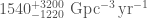


 and
and  ), and the black hole they merge to form (
 ), they are all quite similar
 ,
,  ,
, 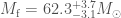 ;
;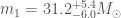 ,
,  ,
,  ;
; ,
,  ,
,  .
. , a particular combination of the two component spins that influences how they inspiral together, and the spin of the final black hole
 ,
,  ;
; ,
,  ;
; ,
, 


 direction. (a) and (b) are the plus and cross tensor polarizations of general relativity. (c) and (d) are the scalar breathing and longitudinal modes, and (e) and (f) are the vector
  and
and  polarizations. The tensor polarizations (in red) are transverse, the vector and longitudinal scalar mode (in green) are longitudinal. The scalar breathing mode (in blue) is an isotropic expansion and contraction, so its a bit of a mix of transverse and longitudinal. Figure 10 from (the excellent)
 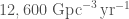 .
.
 is the merger rate, and
  is the surveyed time–volume (you expect more detections if your detectors are more sensitive, so that they can find signals from further away, or if you leave them on for longer). We can estimate
  . We use a uniform prior, for consistency with what we’ve done in the past.
 confidence level limit on the rate is
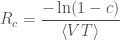 ,
,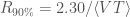
 , the equivalent results is
![\displaystyle R_c = \frac{\left[\mathrm{erf}^{-1}(c)\right]^2}{\langle VT \rangle}](https://s0.wp.com/latex.php?latex=%5Cdisplaystyle+R_c+%3D+%5Cfrac%7B%5Cleft%5B%5Cmathrm%7Berf%7D%5E%7B-1%7D%28c%29%5Cright%5D%5E2%7D%7B%5Clangle+VT+%5Crangle%7D&bg=ffffff&fg=444444&s=0&c=20201002) ,
, , so results would be the same to within a factor of 2, but the results with the uniform prior are more conservative.
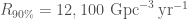 for isotropic spins up to 0.05, and
 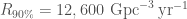 if you allow the spins up to 0.4.
 to
to 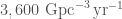 for a 1.4 solar mass neutron star and a black hole between 30 and 5 solar masses and a range of different spins (Table II of the
 and if they all come from neutron star–black hole mergers the angle needs to be bigger than
  .
.
 , and define an effective distance
  defined so that
  where
where  is the analysed amount of time. The plot below show our limits on rate and effective distance for our different injections.
 indicates the spin aligned with the orbital angular momentum. Figure 2 of the
 , we want to know the probability that the parameters
  have different values, which is written as
  . This is calculated using
 ,
, is the likelihood, which we can calculate from our knowledge of the
  is the prior on the parameters (what we would have guessed before we had the data), and the normalisation constant
  is called the evidence. We’ll use the evidence again in the next layer of inference.
 ,
, denotes which model we are considering.
 , we can work this out using another application of Bayes’ theorem (yay)
 ,
, is just all the evidences for the individual events (given that model) multiplied together,
  is our prior for the different models, and
  is another normalisation constant.


 .
. and
and  (where
  is the mass of our Sun), and the final black hole was
  . The quoted values are the median values and the error bars denote the
 . The two-dimensional shows the probability distribution for GW170104 as well as 50% and 90% contours for all events. The one-dimensional plot shows results using different waveform models. The dotted lines mark the edge of our 90% probability intervals. Figure 2 of the
  . GW170104 has similar masses, showing that our first detection was not a fluke, but there really is a population of black holes with masses stretching up into this range.
 qualifies the amount of precession, the way that the orbital plane and black hole
  . Therefore, we disfavour large spins aligned with the orbital angular momentum, but are consistent with small aligned spins, misaligned spins, or spins antialigned with the angular momentum. The value is similar to that for
  .
.

 . The spins of the component black holes are less significant, and can make it a bit higher of lower. We infer a final spin of
  ; there is a tail of lower spin values on account of the possibility that the two component black holes could be roughly antialigned with the orbital angular momentum.
 to
to  , and the uniform in log rate density goes from
  to
to  . The median values stay about the same, but the additional data have shrunk the uncertainties a little.
 at 90% probability. Figure 5 of the GW170104 Supplemental Material (Figure 10 of the
  .
.
 and binary inclination angle
  . The two-dimensional shows the probability distribution for GW170104 as well as 50% and 90% contours. The one-dimensional plot shows results using different waveform models. The dotted lines mark the edge of our 90% probability intervals. Figure 4 of the GW170104 Supplemental Material (Figure 9 of the
  ,
, at different times, and so track how it changes. You can rewrite the equation for the rate of change of the gravitational wave frequency
  , to give an expression for the chirp mass
 .
. are the speed of light and the gravitational constant, which usually pop up in general relativity equations. If you use this formula (perhaps fitting for the trend
  [
[ . The orbital frequency is half this, so
  . The orbital separation
 ![\displaystyle R = \left[\frac{GM}{(2\pi f_\mathrm{orb})^2}\right]^{1/3}](https://s0.wp.com/latex.php?latex=%5Cdisplaystyle+R+%3D+%5Cleft%5B%5Cfrac%7BGM%7D%7B%282%5Cpi+f_%5Cmathrm%7Borb%7D%29%5E2%7D%5Cright%5D%5E%7B1%2F3%7D&bg=ffffff&fg=444444&s=0&c=20201002) ,
, is the binary’s total mass. This formula is only strictly true in
  . We now want to compare the binary’s separation to the size of black hole with the same mass. A
  .
. . A compactness of
  could only happen for black holes. We could maybe get a binary made of two neutron stars to have a compactness of
  , but the system is too heavy to contain two neutron stars (which have a maximum mass of about
  ). The system is so compact, it must contain black holes!
 , the lighter black hole
  and the final black hole (resulting from the coalescence)

 means the binary is face on,
  means it face off, and an inclination around
  is edge on. The bands show the recovered 90% credible interval; the dark lines the median values, and the dotted lines show the true values. The (grey) polarization angle
  was chosen so that the detectors are approximately insensitive to the
  polarization. Figure 4 of the
  and ignores earlier cycles. The standard analysis includes data down to
  , and this extra data does give you a little information about precession. (The limit of the simulation length also means you shouldn’t expect this type of analysis for the longer LVT151012 or GW151226 any time soon).
![\displaystyle L \propto \exp \left[- \int_{-\infty}^{\infty} \mathrm{d}f \frac{|s(f) - h(f)|^2}{S_n(f)} \right]](https://s0.wp.com/latex.php?latex=%5Cdisplaystyle+L+%5Cpropto+%5Cexp+%5Cleft%5B-+%5Cint_%7B-%5Cinfty%7D%5E%7B%5Cinfty%7D+%C2%A0%5Cmathrm%7Bd%7Df+%C2%A0%5Cfrac%7B%7Cs%28f%29+-+h%28f%29%7C%5E2%7D%7BS_n%28f%29%7D+%C2%A0%5Cright%5D&bg=ffffff&fg=444444&s=0&c=20201002) ,
, is the signal,
  is our waveform template and
  is the noise spectral density (
 is accurate. I think that the denominator
  . You need proper templates for the gravitational wave signal to calculate this. If you factor in the the gravitational wave gets redshifted (shifted to lower frequency by the expansion of the Universe), then the true chirp mass of the source system is
  .
. —the total mass of the binary,
  —the chirp mass, the combination of the two component masses which sets how the binary inspirals together;
 —the mass ratio,
  . Confusingly, numerical relativists often use the opposite convention
  (which is why the
  : we can keep the standard definition, but all the numbers are numerical relativist friendly).
 , where
  is the true, redshift-corrected source-frame mass and
  would be now);
 —the inclination, the angle between the line of sight and the orbital angular momentum (
 ). This is zero for a face-on binary.
 ) and the total angular momentum of the binary (
 ); this is approximately equal to the inclination, but is easier to use for precessing binaries.
 (no spin) and
  (maximum spin);
 —the primary tilt angle, the angle between the orbital angular momentum and the heavier black holes spin (
 ). This is zero for aligned spin.
 —the secondary tilt angle, the angle between the orbital angular momentum and the lighter black holes spin (
 ).
). —the angle between the projections of the two spins on the orbital plane.
 —the polarization angle, this is zero when the detector arms are parallel to the
  to
to  .
.
 for some reason. After the introduction, it does get technical, so it’s probably only for insomniacs. However, if you like a good conspiracy and think we might be hiding something, the appendices go through all the details of removing instrumental noise and checking outliers found by the search.
 . The true location is marked by the cross. Leo poetically described this as looking like the seeds of the
  can be approximated using an ansatz
![\displaystyle p(D|\mathrm{data}) \propto D^2\exp\left[-\frac{(D - \mu)^2}{2\sigma}\right]](https://s0.wp.com/latex.php?latex=%5Cdisplaystyle+p%28D%7C%5Cmathrm%7Bdata%7D%29+%5Cpropto+D%5E2%5Cexp%5Cleft%5B-%5Cfrac%7B%28D+-+%5Cmu%29%5E2%7D%7B2%5Csigma%7D%5Cright%5D&bg=ffffff&fg=444444&s=0&c=20201002) ,
, and
and  are calculated for each pixel individually. The form of this ansatz can be understood as the
  , and the likelihood can often be well approximated as a Gaussian distribution, which gives the other piece [