Second year physics undergraduates at the University of Birmingham have to write an essay as part of their course. As a tutor, it’s my job to give them advice on how to write in a scientific style (and then mark the results). I have assembled these tips to try to aid them (and make my marking less painful). Much of this advice also translates to paper writing, and I try to follow these tips myself.
Writing well is difficult. It requires practice. It is an important skill, yet it is something that I do not believe is frequently formally taught (at least in the sciences). Scientific and other technical writing can be especially hard, as it has its own rules that can be at odds with what we learn at school (when studying literature or creative writing). Reading the work of others is a good way for figuring out what works well and what does not.
In this post, I include some tips that I hope are useful (not everyone will agree). I begin by considering how to plan and structure a piece of writing (section 1), from the largest scale (section 1.2) progressing down to the smallest (section 1.4); then I discuss various aspects of technical writing (section 2), both in terms of content and style, including referencing (section 2.5), which is often problematic, and I conclude with some general editing advice (section 3) before summarising (section 4). If you have anything extra to add, please do so in the comments.
1 Structure and planning
The structure of your writing is important as it reflects the logical flow of your arguments. It is worth spending some time before you start writing considering what you want to say, and what is the best order for your ideas. (This is also true in exams: I have found when trying to answer essay questions it is worth the time to spend a couple of minutes planning, otherwise I am liable to miss out an important point). I frequently get frustrated that I must write linearly, one idea after another, and cannot introduce multiple strands at a time, with arguments intertwining with each other. However, putting in the effort to construct a clear progression does help your reader.
1.1 Title and audience
The first thing to consider is what you want to write and who is going to read it. Always write for your audience, and remember that professional scientists and the general public look for different things (this blog may be a poor example of this, as different posts are targeted towards different audiences).
Having thought about what you want to say, pick a title that reflects this. Don’t have a title “The life and works of Albert Einstein” if you are only going to cover special relativity, and don’t have a title “Equilibrium thermodynamics of non-oxide perovskite superconductors” if you are writing for a general audience. If your title is a question, make sure you answer it. It might be a good idea to write your title after you have finished your main text so that you can match it to what you have actually written.
1.2 Beginning, middle and end
To help your audience understand what you are telling them, begin with an introduction, and end with a summary. This is also true when giving a talk. Start by explaining what you will tell them, then tell them, then tell them what you told them. Repetition of key ideas makes them more memorable and help to emphasise what your audience should take away.
At the beginning, introduce the key ideas you will talk about. If you are writing an essay titled “The Solar Neutrino Problem“, you should explain what a solar neutrino is and why there is a problem. You might also like to explain why the reader should care. Sketching out the contents of the rest of the work is useful as it prepares the reader for what will follow: it’s like warm-up stretches for the mind. The introduction sets the scene for the arguments to follow.
The main body of your text contains most of the information, this is where you introduce your ideas and explain them. It is the burger between the buns of the introduction and conclusion. For longer documents, or subjects with many aspects, you might consider breaking this up into sections (and subsections). Using headings (perhaps numbered for reference) is good: skimming section headings should give an outline of the contents. Some sections within the main body might be sufficiently involved to merit their own introduction and summary. There should be a clear progression of ideas: if you find there is a big jump, try writing some text to cover the transition (“Having explained how neutrinos are produced in the Sun, we now consider how they are detected on the Earth”).
After presenting your arguments, it is good to summarise. As an example, a summary on the solar neutrino problem could be:
“Experiments measuring neutrinos from the Sun only detected about a third as many as expected. This could indicate either a problem with our understanding of solar physics or of particle physics. It is not possible to modify solar models to match both the measured neutrino flux and observations of luminosity and composition; however, the reduced flux could be explained by introducing neutrino oscillations. These were subsequently observed in several experiments. The solar neutrino problem has therefore been resolved by introducing new particle physics.”
Don’t introduce new arguments at this stage, this is just as unsatisfying as reading a murder mystery and discovering the murderer was someone never mentioned before. In my solar neutrino example, both the solar models and neutrino oscillations should have been discussed. Distilling your argument down to few lines also helps you to double-check your logic.
Either as part of your summary, of following on from it, end your writing with a conclusion. This is what you want your audience to have learnt (it should be the answer to your question). It is OK if you cannot produce a concrete answer, there are many cases where there is no clear-cut solution, perhaps more data is needed: in these cases, your conclusion is that there is no simple answer. To check that you have successfully wrapped things up, try reading just your introduction and conclusion; these should pair up to form a delicious (but bite-sized) sandwich.
1.3 Paragraphs
On a smaller scale, your writing is organised using paragraphing. Paragraphs are the building blocks of your arguments; each paragraph should address a single point or idea. Big blocks of text are hard to read (and look intimidating), so it is good to break them up. You can think of each paragraph as a micro-essay: the first sentence (usually) introduces the subject, you then go on to elaborate, before reaching a conclusion at the end (see section 1.2). To check that your paragraph sticks to a single point (and doesn’t need to be broken up), try reading the first and last sentences, usually they should make sense together.
1.4 Sentences
Paragraphs are constructed from sentences. Ensure your sentences make sense, that they are grammatically correct and that their subject is clear.
Vary your sentence length. In technical writing there is often the temptation, even amongst the best writers, to include long, convoluted sentences in order to fully describe a complicated idea and include all the relevant details, but these can be hard to read, both because of the complexity of their structure, which may require significant mental effort to unpack, and because by the time they finally conclude, the reader has forgotten the initial topic of the over-long, rambling sentence. Brevity gives impact. Shorter sentences are easier to understand. Breaking up your ideas helps the reader. Short sentences also get boring. They seem repetitive. They are tiring to read. They can send your reader to sleep. It is, therefore, better to have a range of sentence lengths. Include some short. In addition to these, have some longer sentences, as these allow you to join up your ideas. If you are unsure where to break up long sentences, look for commas (or semi-colons, etc.); if you are unsure where to put commas, read the sentence and see where you would pause.
2 Writing style and referencing
Having discussed how to structure your writing, we now move on to what to write. Technical writing has some specific requirements with regards to content, these might seem peculiar when first encountered. I’ll try to explain why we do certain things in technical writing, and give some ideas on how to incorporate these ideas to improve your own writing.
2.1 Be specific
The most common mistake I come across in my students’ work is the failure to be specific. The following two points (sections 2.2 and 2.3) are closely related to this. As an example, consider making a comparison:
- Poor — “Nuclear power provides more energy than fossil fuel.”
- Better — “Per unit mass of fuel, nuclear fission releases more energy than the burning of fossil fuel.”
- Even better — “Nuclear fission can produce ~8000 times as much energy per unit mass of fuel as burning fossil fuels: the same amount of energy is produced from 16 kg of fossil fuels as by using 2 g of uranium in a standard reactor (MacKay, 2008).”
Here, we have specified exactly what we are comparing, given figures to allow a quantitative comparison, and provided references for those figures (see section 2.5). If possible, give numbers; don’t say “many ” or “lots” or “some”, but say “70%”, “9 billion” or “six Olympic swimming pools”.
Weak modifiers like “very”, “quite”, “somewhat” or “highly” are another example where it is better to be specific. What is the difference between being “hot” and being “very hot”? I might say that my bowl of soup is very hot, but does that tell you any more than if I just said it was hot? It is tempting to use these words for emphasis, surely if I were talking about the surface of the Sun we can agree that’s very hot? Not if you were to compare it to the centre of the Sun! Often, what is hot or cold, big or small, fast or slow depends upon the context. What is hot for soup is cold for the Sun, and what is cold for soup is hot for superconductors. It is much better to make distinctions by using figures: “The surface of the Sun is about 6000 K”.
It is OK to use “very” if you define the range where this is applicable, for example “High frequency radio waves are between 3 MHz and 30 MHz, very high frequency radio waves are between 30 MHz and 300 MHz, and ultra high frequency radio waves are between 300 MHz and 3 GHz.”
2.2 Provide justification
When putting forward an argument, it is necessary to include some evidence or justification to back it up. It is not sufficient merely to assert your opinion because you need the reader to follow your reasoning. If you are using someone else’s argument, you should provide a citation (section 2.5); the reader can then check there to find the reasoning. However, if it is an important point you might like to add some exposition. If you are being good about providing quantitative statements (section 2.1), you are already part way there as you can use those figures a back-up. For example, if discussing global warming, it is easy to argue it is important if you have already included figures on how many people would lose their homes to rising sea-levels, or if comparing materials, it is straightforward to argue that aluminium is better for making aeroplanes than steel if you have already included their densities. Sometimes, all that is required is an explanation of your reasoning, for example, “It is a good idea to build nuclear power plants because this reduces reliance on fossil fuels” or “It is not advisable to lick the surface of the Sun because it doesn’t taste of golden syrup.” Here, the reader might disagree that it is a good idea to build nuclear power plants, but they understand that you are using dependence on fossil fuels as an argument instead of, say, environmental issues, or the reader might agree that it is a bad idea to lick the Sun, but might have been thinking more about its temperature than its flavour. Even if the reader does not agree with your conclusions, they should understand how you reached them.
A similar idea is to show rather than tell. Don’t tell me that something is a fascinating topic or an exciting concept, get on with explaining it! Similarly, don’t just say something is important, but explain why it is important. This allows the reader to decide upon things themselves, if you have justified your arguments then they should follow your logic.
2.3 Use the correct word
In technical writing there is often a specific word that should be used in a particular context. In common usage we might use weight and mass interchangeably, in physics they have different meanings. This sometimes trips people up as they naturally try to find synonyms to reduce the monotony of their work. Always use the correct term.
Technical language can be full of jargon. This makes things difficult to understand for an outsider. It is important to define unfamiliar terms to help the reader. In particular, acronyms must be defined the first time they are used. As an example, “When talking about online materials, the uniform resource locator (URL), otherwise known as the web address, is a string of characters that identifies a resource.” Avoid jargon as much as possible; try to always use the simplest word for the job. It will be necessary to use technical terms to describe things accurately, but if they are introduced carefully, these need not confuse the reader.
A particular pet-peeve of mine is the use of scare quotes, which I always read as if the author is making air quotes. If quoting someone else’s choice of phrase then quotation marks are appropriate, and a reference must be provided (section 2.5). Most of the time, these quotation marks are used to indicate that the author thinks the terminology isn’t quite right. If the terminology is incorrect, use a different word (the correct one); if the terminology is correct (if that is what is used in the field), then the quotation marks aren’t needed!
Most physics problems involve solving an equation or two. For these mathematical questions, I am always encouraging my students to explain their work, to use words. When writing essays, I find they have the opposite problem: they only use prose and don’t include equations (or diagrams). Equations are useful for concisely and precisely explaining relationships, it is good to include them in writing.
Equations may put off general readers, but they improve the readability of technical work. Consider describing the kinetic energy of a (non-relativistic) particle:
- With only words — “The kinetic energy of a particle depends upon its mass and speed: it is directly proportional to the mass and increases with the square of the speed.”
- Using an equation — “The kinetic energy of a particle
 is given by
  , where
  is its mass and
  is its velocity.”
The second method is more straightforward, there is no ambiguity in our description, and we also get the factor of a half so the reader can go away at calculate things for themselves. This was just a simple equation; if we were considering something more complicated, such as the kinetic energy of a relativistic particle
 ,
,
where  is the speed of light, it is much harder to produce a comprehensive description using only words. In this case, it is tempting to miss out reference to the equation. Sometimes this is justified: if the equation is too complicated a reader will not understand its meaning, but, in many cases, an equation allows you to show exactly how a system changes, and this is extremely valuable.
When including an equation, always define the symbols that you are using. Some common constants, such as  , might be understood, but it is better safe than sorry.
Equations should be correctly punctuated. They are read as part of the surrounding text, with the equals sign read as the verb “equals”, etc.
Using diagrams is another way of providing information in a clear, concise format. Like equations, diagrams can replace long and potentially confusing sections of text. Diagrams can be pictures of experimental set-up, schematics of the system under discussion, or show more abstract information, such as illustrating processes (perhaps as a flow chart). The cliché is that a picture is worth a thousand words; as diagrams are so awesome for conveying information, I’m not even going to attempt to give an example where I try to use only words. Below is as example figure, which I have chosen as it also includes equations.
“Figure 1 shows the proton–proton (pp) chain, the series of thermonuclear reactions that provides most (~99%) of Sun’s energy (Bahcall, Serenelli & Basu, 2005). There are several neutrino-producing reactions.”

Figure 1: The thermonuclear reactions of the pp chain. The traditional names of the produced neutrinos are given in bold and the branch names are given in parentheses. Percentages indicate branching fractions. Adapted from Giunti & Kin (2007).
Graphs can be used to show relationships between quantities, or collections of data. They can be used for theoretical models or experimental results. In the example below I show both. Graphs might be useful for plotting especially complicated functions, where the equation isn’t easy to understand. There are many types of graph (scatter plots, histograms, pie charts), and picking the best way to show your data can be as challenging as obtaining it in the first place!
“In figure 2 we plot the orbital decay of the Hulse–Taylor binary pulsar, indicated by the shift in periastron time (the point in the orbit where the stars are closest together). The data are in excellent agreement with the prediction assuming that the orbit evolves because of the emission of gravitational waves.”

Figure 2: The cumulative shift of periastron time as a function of time of the Hulse–Taylor binary pulsar (PSR B1913+16). The points are measured values, while the curve is the theoretical prediction assuming gravitational-wave emission. Taken from Weisberg & Taylor (2005).
All diagrams should have a descriptive caption. It is usually good to number these for ease of reference. If you are using someone else’s figure, make sure to explicitly cite them in the caption (see section 2.5)—you need to unambiguously acknowledge that you have taken someone else’s work, and have not just used their data or ideas (which would also warrant a citation) to make your own.
Tables can also be used to present data. Tables might be better than plots for when there are only a few numbers to present. Like figures, tables should have a caption (which includes relevant references if the data is taken from another source), they should be numbered, and they should be referred to explicitly in the text.
When writing, it is useful to remember that different people learn better through different means: some prefer words, some love equations, and other like visual representations. Including equations and figures can help you communicate effectively with a wider audience.
There are conventions for how to present equations, graphs and tables. I shall return to this in future posts. The rules may seem arcane, but they are designed to make communication clear.
2.5 Referencing
At the end of any good piece of technical writing there should be a list of references, hence I have tackled referencing last in the section. (Sometimes this is done in footnotes rather than the end, but I’m ignoring that). However, referencing should not be considered something that is just done at the end, or something that is tacked on at the end as an after-thought; it is one of the most important components of academic writing.
We include references for several reasons:
- To show the source of facts, figures and ideas. This allows readers to verify things that we quote, to double-check we’ve not made an error or misinterpreted things. It also shows distinguishes what is our own from what we have taken from elsewhere. This is important in avoiding plagiarism, as we acknowledge when we use someone else’s work.
- To provide the reader with a further source of information. It is not possible to explain everything, and a reader might be interested in finding out more about a topic, how a particular quantity was measured or how a particular calculation was done. By providing a reference we give the reader something further they can read if they want to (that doesn’t mean our work shouldn’t make sense on it’s own: you should be able to watch The Avengers without having seen Iron Man, but it’s still useful to know what to watch to find out the back-story). By following references readers can see how ideas have developed and changed, and gain a fuller understanding of a topic.
- To give credit for useful work. This is linked to the idea of not claiming the ideas as your own (avoiding plagiarism), but in addition to that, by referencing something you are publicising it, by using it you are claiming that it is of good-enough quality to be trusted. If you are to look at an academic article you will often see a link to citing articles. The number of citations is used as a crude measure of the value of that paper. Furthermore, this linking can allow a reader to work forwards, finding new ideas built upon those in that paper, just as they can work backwards by following references.
- To show you know your stuff. This might sound rather cynical, but it is important to do your research. To understand a topic you need to know what work has been done in that area (you can’t always derive everything from first principles yourself), and you demonstrate your familiarity with a field by include references.
You must always include citations in the text at the relevant point: if you use an idea include your source, if you introduce a concept say where it came from. It is not acceptable just to have a list of references at the end: does the reader have to go through all of these to figure out what came from where?
There are multiple styles for putting citations in text. The two most common are the following:
- Numeric (or Vancouver) — using a number, e.g., [1], where the references at the end form an ordered list. This has the advantage of not taking up much space, especially when including citations to multiple papers, e.g. [1–5].
- Author–year (or Harvard) — using the authors and year of publication to identify the paper, e.g., (Einstein, 1905). This has the advantage of making it easier to identify a paper: I’ve no idea what [13] is until I flick to the end, but I know what (Hulse & Taylor, 1975) is about.
Which style you use might be specified for you or it might be a free choice. Whichever style you use, the important thing is to include relevant references at the appropriate place in the text.
Having figured out why we should reference, where we should put references and how to include citations in the text, the last piece is how to assemble the bibliographic information to include at the end (or in footnotes). Exactly what information is included and how it is formatted depends on the particular style: there are endless combinations. Again, this might be specified for you or might be a free choice, just make sure you are consistent. Basic information that is always included are an author (this may be an organisation rather than a person), so we know who to attribute the work to, and a date so we know how up-to-date it is. Other information that is included depends upon the source we are referencing: a journal article will need the name of the journal, the volume and page number; a book will need a title, edition and publisher; a website will need a title and URL, etc. We need to include all the necessary information for the reader to find the exact source we used (hence we need to include the edition of a book, the date updated or written for a website, and so on).
There are numerous guides online for how to format references correctly. Some software does it automatically (I use Mendeley to produce BibTeX, but that’s not for everyone). The University of Birmingham has a guide to using Havard-style referencing that is comprehensive.
A final issue remains of which sources to reference: how do you know that a source is reliable? This is an in-depth question, so I shall return to it is a dedicated post.
3 Editing
Writing isn’t finished as soon as you have all your ideas on the page, things often take some polishing up. Some people like to perfect things as they go along, others prefer to get everything down in whatever form and go back through after. Here, I conclude with some tips for editing.
3.1 Be merciless
Keep your writing short. Don’t waste your readers’ time or overcomplicate things. Cut unnecessary words.
There are some phrases that are typically superfluous:
- “Obviously…” — If it is obvious, then the reader will realise it; if it’s not, you are patronising them.
- “It should be noted that…” — That would be why it’s written down! (I hope you are not writing things that shouldn’t be noted).
- “Remember that…” — You’re reminding the reader by writing it.
- Any of the modifiers like “very”, “quite” or “extremely” mentioned in the section 2.3.
3.2 Proof-read
The single best method to improve a piece of writing is to proof-read it. Reread what you have written to check that it says what you think it should. I find I have to wait for a while after writing something to read it properly, otherwise I read what I intended to write rather than what I actually did. Having others read it is an excellent way to check it makes sense (especially if you are not a native English speaker); this is best if they are representative of your target audience.
I hate it when others find a mistake in my writing. It’s like rubbing a cat the wrong way. However, each mistake you find and correct makes your writing a little better, and that’s really the important thing.
4 Summary
In conclusion, my main tips for good scientific writing are:
- Plan what you want to tell your audience and how they will take your message away.
- Say what you’re going to say (introduction), then say it (main text), then say what you said (conclusion).
- Have a clear, logical flow, with one point per paragraph.
- Be specific and back up with your points with quantitative data and references.
- Use equations and diagrams to help explain.
- Be concise.
- Proof-read (and get a second opinion).
If you have any further ideas for improving essay writing, please leave a comment.


 to mean the probability of
  . A joint probability describes the probability of two (or more things), so we have
  as the probability that both
  happen. The probability that
  . Consider the the joint probability of
  .
. .
. .
. ,
, . We normally have a model that can predict how likely it would be to observe that data if our hypothesis is true, so we know
  , so we just need to convert between the two. This is known as the inverse problem.
 .
. is the prior, because it’s what we believed about our hypothesis before we got the data, and
  is the evidence. If ever you hear of someone doing something in a Bayesian way, it just means they are using the formula above. I think it’s rather silly to point this out, as it’s really the only logical way to do science, but people like to put “Bayesian” in the
  .
. . The prior probability of not having the disease is
  . The likelihood of our positive result is
  , which seems worrying. The evidence, the total probability of testing positive
  is found by adding the probability of a true positive and a false positive
 .
. . We thus have everything we need. Substituting everything in, gives
 .
.
 .
. . If we assume that it is equally likely that any one of the children opened the door, then the likelihood that one of the girls did so when their are two of them is
  . Similarly, if there were two boys, the probability of a girl answering the door is
  . The evidence, the total probability of a girl being at the door is
 .
. .
. .
. , makes a difference. We know the probability of surviving the fatal dose is
  . The evidence, the total probability of surviving
  , is calculated by considering the two possible sequence of events: either Ted ate the fudge and survived or he didn’t eat the fudge and survived
 .
. . Since Ted either ate the fudge or he didn’t
  . Therefore,
![P(\mathrm{survive}) = 0.5 P(\mathrm{fudge}) + [1 - P(\mathrm{fudge})] = 1 - 0.5 P(\mathrm{fudge})](https://s0.wp.com/latex.php?latex=P%28%5Cmathrm%7Bsurvive%7D%29+%3D+0.5+P%28%5Cmathrm%7Bfudge%7D%29+%2B+%5B1+-+P%28%5Cmathrm%7Bfudge%7D%29%5D+%3D+1+-+0.5+P%28%5Cmathrm%7Bfudge%7D%29&bg=ffffff&fg=444444&s=0&c=20201002) .
. .
. . In this case,
 .
. . In this case we are in a state of ignorance. Our posterior is
 .
. .
. . Then
 .
.


 ,
, is the black hole’s mass (as it increases, so does the size of the event horizon);
  is
is  ). You can plug in some numbers to this formula (if anything like me, two or three times before getting the correct answer), to find out how big a black hole is (or equivalently, how much you need to squeeze something before it will collapse to a black hole).
 .
. . An interesting consequence of this (well, something I think is interesting), is to consider the effective density of a black hole. Density is how much mass you can fit into a given space. In our case, we’ll consider the mass of the black hole and the volume of its event horizon. This would be something like
 ,
, for density and you shouldn’t worry about the factors of

 as shorthand for the mass of the Sun (one solar mass). This particular X-ray source is peculiarly bright and has long been suspected to potentially be a black hole with a mass around
  to
to  . If the result is confirmed, then it is the first definite detection of an intermediate-mass black hole, or IMBH for short, but why is this exciting?
 , known as the
  and
and  . After this, nothing can resist gravity and you end up with a black hole of a few times the mass of the Sun.
 to
to  . The strongest evidence comes from our own galaxy, where we can
  ). These correlations tell us that the evolution of the galaxy and it’s central black hole are linked somehow, this could be just because of their shared history or through some extra feedback too.
 ,
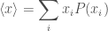
,  , etc., or as
  where the subscript
  is used as shorthand to indicate any of the possible outcomes. The probability of the numeric value being a particular
  . For rolling our dice, the outcomes are one to six (
 ,
,  , etc.) and the probabilities are
 .
. ,
, means
means  .
.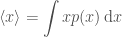 ,
, is the probability density function.
 ,
, is less than one, so if
  , it’s worth playing. If we were tossing a (fair) coin, we’d expect to come out even, if we had to roll a six, we’d expect to pay more.
 . Imagine each outcome
  times, then the mean is
 .
. so that
  .
. . This can be done by adding up probabilities until you get a half
 .
. ,
, is the lower limit of the distribution. (That’s all the calculus out of the way now, so if you’re not a fan you can relax). The
  .
. .
. and
and  to describe horizontal and vertical position respectively. Cartesian coordinates give you a nice grid with everything at right-angles. Undergrad students often like to stick with Cartesian coordinates as they are straight-forward and familiar. However, they can be a pain when describing a circle. If we want to plot a line five units from the origin of of coordinate system
  , we have to solve
  . However, if we used a
  . By using coordinates that match the symmetry of our system we greatly simplify the problem!

 . By understanding symmetries, we can formulate our analysis of the problem such that we ask the best questions.
 , or if rolling a die, the probability of getting a six is
  .
. is given by the
  .
. , we would calculate
 .
. .
. ).
). .
. .
. is the probability of
  given that
  . If I told you that I have rolled a six, then the probability of me having rolled an even number is
  —it’s a dead cert, so bet all your fudge on that! When combining probabilities from dependent events, we chain probabilities together in a logical chain. The probability of rolling a six and an even number is the probability of rolling an even number multiplied by the probability of rolling a six given that I rolled an even number
 ,
, .
. .
. .
. .
. .
. .
. . The probability of not surviving is much easier to work out as there’s only one way that can happen: rolling a six and then overdosing on fudge. The probability is
 ,
, , exactly as before, but in fewer steps.
 , or one in twenty. The probability of rolling two sixes is
  or about one in forty. Hence, you should be almost twice as surprised by rolling double six as for a 95% confidence-level result being incorrect.